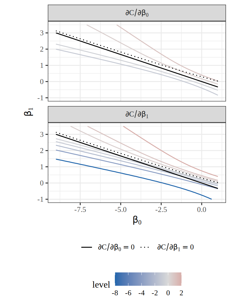
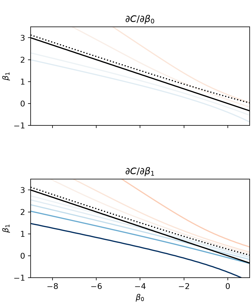
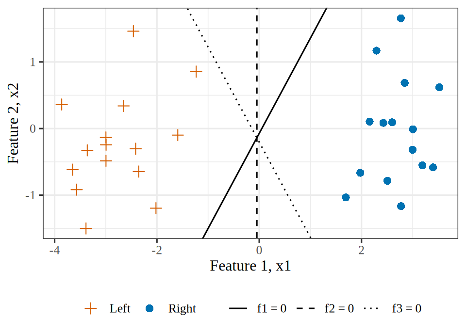
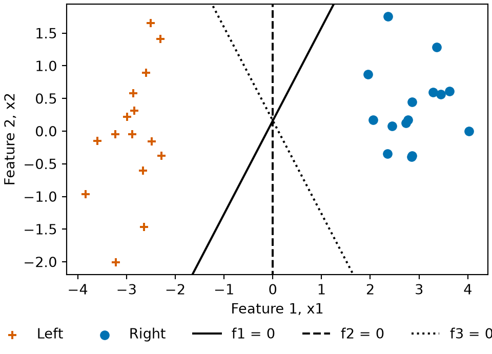
import matplotlib.pyplot as plt
import numpy as np
from matplotlib.colors import LogNorm

x_obs = np.array([1, 2, 4, 5])
y_obs = np.array([0, 0, 1, 1])


def cost_and_grad(b0, b1):
    z = b0[..., None] + b1[..., None] * x_obs
    resid = 1 / (1 + np.exp(-z)) - y_obs
    cost = (np.logaddexp(0, z) - y_obs * z).sum(axis=-1)
    return cost, resid.sum(axis=-1), (resid * x_obs).sum(axis=-1)


b0, b1 = np.meshgrid(np.linspace(-9, 1, 101), np.linspace(-1, 3.5, 46))
cost, _, _ = cost_and_grad(b0, b1)
a0, a1 = np.meshgrid(np.arange(-9, 2), np.arange(-1, 4))
_, d0, d1 = cost_and_grad(a0.astype(float), a1.astype(float))
norm = np.hypot(d0, d1)
fig, ax = plt.subplots(figsize=(4.5, 3.5), layout="constrained")
# Contours at values of C that double from 1/8 to 16 (see the text).
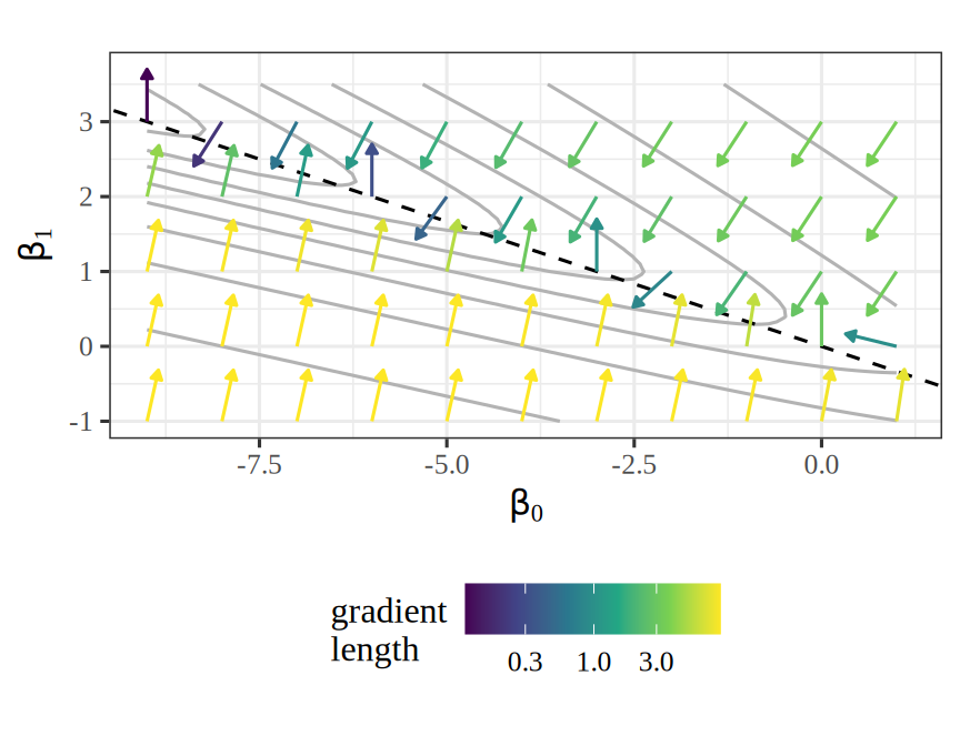
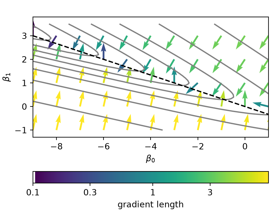
ax.contour(b0, b1, cost, levels=2.0 ** np.arange(-3, 5), colors="grey");
ax.axline((0, 0), slope=-1 / 3, color="black", linestyle="--");
arrows = ax.quiver(a0, a1, -d0 / norm, -d1 / norm, norm, norm=LogNorm(),
                   cmap="viridis", angles="xy", scale_units="xy", scale=1 / 0.7)
bar = fig.colorbar(arrows, ax=ax, location="bottom", label="gradient length")
bar.set_ticks([0.1, 0.3, 1, 3], labels=["0.1", "0.3", "1", "3"]);
bar.minorticks_off();
# Room for the arrows on the top and bottom rows.
ax.set_ylim(-1.3, 3.8);
ax.set_aspect("equal");
ax.set_xlabel(r"$\beta_0$");
ax.set_ylabel(r"$\beta_1$");
plt.show()