Show code
# reticulate provisions the packages this page's Python chunks import.
python_packages <- c("numpy", "pandas", "matplotlib", "scikit-learn")
reticulate::py_require(python_packages)# reticulate provisions the packages this page's Python chunks import.
python_packages <- c("numpy", "pandas", "matplotlib", "scikit-learn")
reticulate::py_require(python_packages)Adapted from Kameron Decker Harris’ 2022 weekly notes, and drawing on Logan Sizemore’s Spring 2025 lecture on decision trees. The Gini index and the reference on classification and regression trees are from the cited sources rather than from that lecture, which uses entropy alone for impurity.
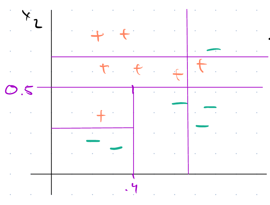
A decision tree partitions the input space into rectangles aligned with the axes. The number of nodes, that is of comparisons, measures the complexity of the tree, and a complex tree overfits.
The parts have names. The topmost node is the root; an internal node, which holds a comparison between one feature and one threshold, is a decision node; a terminal node, which holds a prediction, is a leaf. Applying a decision node’s comparison to send each point down one branch or the other is a split.
Goal:
Keep the tree as compact as possible.
Make the leaves pure.
Finding the optimal tree is NP-hard, so instead we greedily minimize the “impurity” of each split.
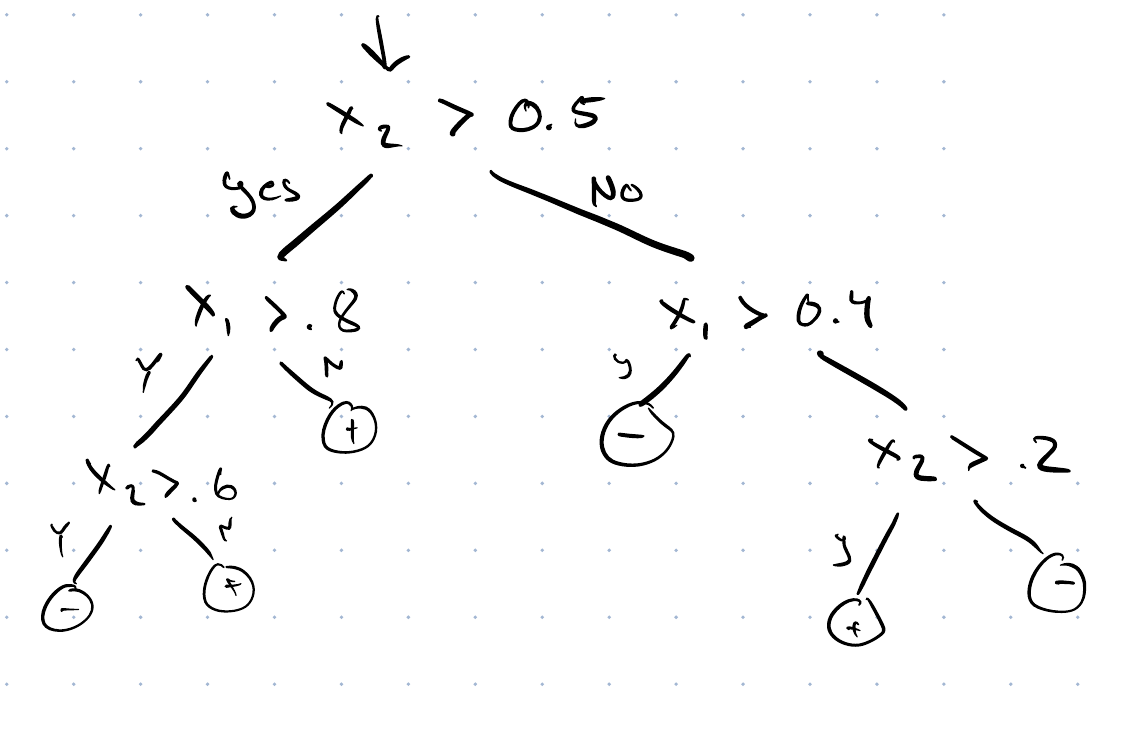
GeeksforGeeks explains decision trees [4].
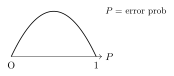
The word “impurity” above is central to the algorithm, so we define it here. A node holding points of one class only is pure; a node holding an even mix of every class is as impure as a node can be. Two standard measures capture exactly this.
Entropy comes from information theory. An outcome of probability \(p\) carries \(-\log_2 p\) bits of surprisal: large when the outcome was unlikely, and zero when it was certain. Predicting heads on a single toss of a fair coin and being right is worth one bit; predicting ten heads in a row and being right is worth \(10\) bits. The population average of the surprisals, weighted by the probabilities themselves, is the entropy [6]:
\[H(S) = -\sumto{k}{C} p_k \log_2 p_k\]
where \(p_k\) is the fraction of the points in the set \(S\) that carry class \(k\), and \(0 \log_2 0\) is read as \(0\). It is zero when one class holds all the mass — there is nothing left to transmit — and largest, at \(\log_2 C\), when the classes are evenly split. So it measures impurity directly: the entropy of a node is the number of bits per point you would still have to send to resolve the labels once the reader knows which leaf a point fell into.
Here are three example nodes. A node holding \(10\) points of each of two classes has \(H = 1\) bit, the worst possible. A node holding \(10\) and \(4\) has \(H = 0.863\). A node holding \(10\) and \(0\) has \(H = 0\).
Gini impurity is the other standard choice:
\[G(S) = 1 - \sumto{k}{C} p_k^2\]
It is the probability that two points drawn independently from \(S\) carry different labels — equivalently, the error rate you would get by labeling a point at random from \(S\)’s own class proportions. It agrees with entropy at both ends, zero for a pure node and largest for an even mix, and differs only mildly in between, so the choice between the two rarely changes the tree that comes out. Entropy is the criterion of Quinlan’s ID3 [7]; Gini is the default in the classification and regression tree procedure of Breiman, Friedman, Olshen and Stone [8].
GeeksforGeeks explains Gini impurity and entropy [10].
A split sends the points of \(S\) into \(B\) branches \(S_1, \dots, S_B\) — \(B = 2\) for a yes-or-no comparison on one feature. Score it by how much impurity it removes. The impurity left afterwards is each branch’s impurity weighted by the share of the points that landed in it, and the information gain is the difference, which is the mutual information between a point’s branch and its class:
\[\mathrm{IG}(S, \text{split}) = H(S) - \sumto{b}{B} \frac{|S_b|}{|S|}\, H(S_b)\]
The weighted sum stops the greedy rule from being misled. Separating one point into its own branch makes that branch perfectly pure, but it arrives with weight \(1/|S|\) and leaves the other branch almost exactly as impure as the parent was, so the gain is negligible. The rule rewards a split for purifying a large share of the data, not for purifying something.
Growing the tree is then a loop: at each leaf, try every feature and every valid threshold, compute the gain for each candidate, keep the largest, and recurse on the branches it creates.
GeeksforGeeks explains information gain [12].
Exercise 1 (Compute the entropy of a skewed distribution) A node holds points of four classes, in the proportions \(p = (\tfrac{1}{2}, \tfrac{1}{4}, \tfrac{1}{8}, \tfrac{1}{8})\). Compute its entropy \(H\) in bits, by hand.
Exercise 2 (Compare with the uniform distribution) Now take the same four classes in equal proportions, \(p = (\tfrac{1}{4}, \tfrac{1}{4}, \tfrac{1}{4}, \tfrac{1}{4})\). Compute \(H\).
Exercise 3 (Compare with the uniform distribution (part 2)) Use the setup of Exercise 2.
Compare \(H\) with that of Exercise 1.
Exercise 4 (Compare with the uniform distribution (part 3)) Use the setup of Exercise 2.
Which node is easier to describe, and why?
Exercise 5 (Compute the entropy at the root of a small tree) A training set holds all eight combinations of three binary features \(x_1, x_2, x_3 \in \{0, 1\}\), labeled by the rule \(y = 1\) if both \(x_1 = 1\) and \(x_2 = 1\), and \(y = 0\) otherwise. The feature \(x_3\) plays no part in the rule.
What is the entropy of the labels at the root, before any split?
Exercise 6 (Choose the first split by information gain) For the data of Exercise 5, compute the information gain of splitting on each of \(x_1\), \(x_2\) and \(x_3\).
Exercise 7 (Choose the first split by information gain (part 2)) Use the setup of Exercise 6.
Which feature, or features, would the greedy rule split on first?
Exercise 8 (Finish the tree) Split on \(x_1\) first, as the gains in Exercise 6 allow. Which branch is already pure?
Exercise 9 (Finish the tree (part 2)) Use the setup of Exercise 8.
For the other branch, compute the information gain of each remaining feature.
Exercise 10 (Finish the tree (part 3)) Use the setup of Exercise 8.
Finish the tree that splits on \(x_1\) first.
Exercise 11 (Finish the tree (part 4)) Use the setup of Exercise 8.
How many leaves does the finished tree have?
Exercise 12 (Finish the tree (part 5)) Use the setup of Exercise 8.
Does the finished tree classify all eight training points correctly?
The same procedure fits numeric targets once we change the impurity measure. A leaf predicts the sample mean of the training targets it holds,
\[\hy_S = \frac{1}{|S|}\sum_{i \in S} y_i\]
so we measure a node’s impurity by how far its targets spread around that sample mean:
\[V(S) = \frac{1}{|S|}\sum_{i \in S}\paren{y_i - \hy_S}^2\]
Putting \(V\) in place of \(H\) in the expression above gives the variance reduction of a split,
\[\mathrm{VR}(S, \text{split}) = V(S) - \sumto{b}{B} \frac{|S_b|}{|S|}\, V(S_b)\]
and a regression tree splits to maximize it. Because the leaf predicts the sample mean, \(|S|\,V(S)\) is exactly the squared error that leaf would incur, so maximizing variance reduction is minimizing training squared error one split at a time.
hitters_all <- readr::read_csv("data/hitters.csv", show_col_types = FALSE)
hitters_tree_data <- hitters_all[!is.na(hitters_all$Salary), ]
hitters_tree_data$log_salary <- log(hitters_tree_data$Salary)
# Grow the tree with no stopping rule,
# then keep the best subtree with two splits.
grow_all <- rpart::rpart.control(cp = 0, minsplit = 2)
hitters_big <- rpart::rpart(
  log_salary ~ Years + Hits,
  data = hitters_tree_data,
  control = grow_all
)
two_splits <- hitters_big$cptable[, "nsplit"] == 2
has_two_splits <- any(two_splits)
stopifnot(has_two_splits)
cp_two_splits <- hitters_big$cptable[two_splits, "CP"]
hitters_tree <- rpart::prune(hitters_big, cp = cp_two_splits)
plot(hitters_tree, margin = 0.1)
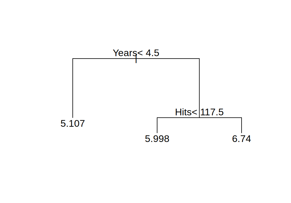
text(hitters_tree, digits = 4)Years) and the number of hits in the previous season (Hits). Each split sends a player who meets its condition to the left. Each leaf shows the sample mean log salary of the players in it.
import numpy as np
import pandas as pd
import matplotlib.pyplot as plt
from sklearn.tree import DecisionTreeRegressor, plot_tree

hitters = pd.read_csv("data/hitters.csv").dropna(subset=["Salary"])
X_hitters = hitters[["Years", "Hits"]]
y_hitters = np.log(hitters["Salary"])
# Best-first growth with three leaves keeps the two splits that reduce
# the squared error most.
hitters_tree = DecisionTreeRegressor(max_leaf_nodes=3, random_state=0)
hitters_tree.fit(X_hitters, y_hitters);
fig, ax = plt.subplots(figsize=(8, 4.5));
plot_tree(hitters_tree, feature_names=["Years", "Hits"], precision=3, impurity=False, ax=ax);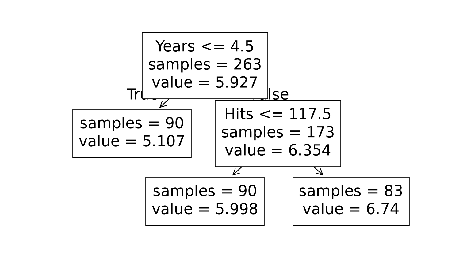
plot(
  hitters_tree_data$Years, hitters_tree_data$Hits,
  pch = 20, col = "grey50", xlab = "Years", ylab = "Hits"
)
abline(v = 4.5, lwd = 2)
right_edge <- max(hitters_tree_data$Years) + 1
segments(4.5, 117.5, right_edge, 117.5, lwd = 2)
region_labels <- tibble::tribble(
  ~x, ~y, ~label,
  2.5, 200, "R1",
  15, 40, "R2",
  15, 220, "R3"
)
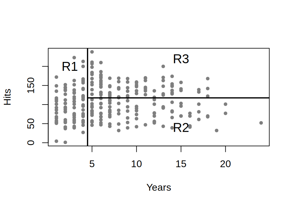
text(region_labels$x, region_labels$y, region_labels$label, cex = 1.3)Years and Hits, with one point per player. \(R_1\) holds the players with fewer than 4.5 years in the major leagues, \(R_2\) the more experienced players with fewer than 117.5 hits, and \(R_3\) the more experienced players with more hits.
fig, ax = plt.subplots(figsize=(5, 3.5));
ax.scatter(hitters["Years"], hitters["Hits"], s=8, color="grey");
ax.axvline(4.5, color="black", linewidth=2);
ax.plot([4.5, hitters["Years"].max() + 1], [117.5, 117.5], color="black", linewidth=2);
for label, x, y in [("R1", 2.5, 200), ("R2", 15, 40), ("R3", 15, 220)]:
    ax.text(x, y, label, fontsize=13);
ax.set_xlabel("Years");
ax.set_ylabel("Hits");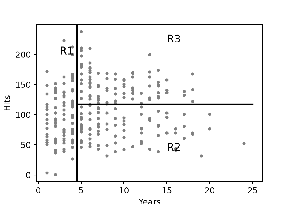
Remark 1 (The tree as a partition of the feature space). The tree of Example 2 cuts the plane of Years and Hits into three regions, drawn in Figure 5:
\[ \begin{aligned} R_1 &= \setbuild{\vx}{\text{Years} < 4.5}, \\ R_2 &= \setbuild{\vx}{\text{Years} \geq 4.5,\ \text{Hits} < 117.5}, \\ R_3 &= \setbuild{\vx}{\text{Years} \geq 4.5,\ \text{Hits} \geq 117.5}. \end{aligned} \]
The regions are the leaves of the tree, which James et al. [13, Sec. 8.1.1] also call “terminal nodes”. They call the decision nodes “internal nodes”, and the segments of the tree that join the nodes “branches”. A tree is drawn upside down, with its root at the top and its leaves at the bottom.
Remark 2 (Reading the baseball salary tree). The tree of Example 2 says that Years matters most for salary: players with less experience earn less than players with more. Among the less experienced players, the previous season’s hits play little part in salary, since the tree does not split their leaf. Among players with five or more years in the major leagues, those with more hits in the previous season tend to earn more.
Three leaves are probably too simple a description of how hits, years and salary are related. Even so, the tree is easier to explain than a linear regression of the same data, and it fits in one small picture [13, Sec. 8.1.1].
Remark 3 (The squared error a regression tree minimizes). Building a regression tree takes two steps [13, Sec. 8.1.1].
For example, with two regions whose training targets have sample means 10 and 20, the tree predicts 10 anywhere in \(R_1\) and 20 anywhere in \(R_2\).
The regions could have any shape. A tree uses boxes, rectangles aligned with the axes, one side per feature, because boxes are simple and a model built from them can be read as a short list of rules. The aim is the boxes whose residual sum of squares is smallest,
\[ \RSS = \sumto{m}{M} \sum_{i \,:\, \vx_i \in R_m} \devof{\outvar_i}{\hy_{R_m}}\sq. \]
There are far too many ways to divide those values into \(M\) boxes to check each one, so a tree is grown one split at a time instead.
# The residual sum of squares after splitting y at each cutpoint of x,
# taken halfway between adjacent values in the data.
split_rss <- function(x, y) { # nolint: function_location_linter
  values <- unique(x)
  values <- sort(values)
  cutpoints <- (head(values, -1) + tail(values, -1)) / 2
  rss <- purrr::map_dbl(cutpoints, function(s) {
    left <- y[x < s]
    right <- y[x >= s]
    left_dev <- left - mean(left)
    right_dev <- right - mean(right)
    sum(left_dev^2) + sum(right_dev^2)
  })
  best <- which.min(rss)
  tibble::tibble(cutpoint = cutpoints[best], rss = rss[best])
}
log_salary <- hitters_tree_data$log_salary
root_dev <- log_salary - mean(log_salary)
root_rss <- sum(root_dev^2)
years_split <- split_rss(hitters_tree_data$Years, log_salary)
hits_split <- split_rss(hitters_tree_data$Hits, log_salary)
first_split <- dplyr::bind_rows(
  Years = years_split,
  Hits = hits_split,
  .id = "feature"
)
first_splitdef split_rss(x, y):
"""The best cutpoint of x for splitting y, and the RSS after it."""
x = x.to_numpy()
y = y.to_numpy()
values = np.unique(x)
cutpoints = (values[1:] + values[:-1]) / 2
rss = []
for s in cutpoints:
left = y[x < s]
right = y[x >= s]
rss.append(((left - left.mean()) ** 2).sum() + ((right - right.mean()) ** 2).sum())
best = int(np.argmin(rss))
return cutpoints[best], rss[best]
pd.DataFrame(
[("Years", *split_rss(hitters["Years"], y_hitters)),
("Hits", *split_rss(hitters["Hits"], y_hitters))],
columns=["feature", "cutpoint", "rss"],
) feature cutpoint rss
0 Years 4.5 115.058475
1 Hits 117.5 160.971530Definition 1 (Recursive binary splitting) Recursive binary splitting grows a regression tree from training data \((\vx_1, \outvar_1), \ldots, (\vx_N, \outvar_N)\). It starts with all \(N\) of them in one region, the root. For a region \(R\), a feature index \(j\) and a cutpoint \(s\), write
\[ R_1(j, s) = \set{\vx \in R : \predvar_j < s}, \qquad R_2(j, s) = \set{\vx \in R : \predvar_j \geq s}. \]
The best split of \(R\) is the pair \((j, s)\) that minimizes
\[ \sum_{i \,:\, \vx_i \in R_1(j, s)} \devof{\outvar_i}{\hy_{R_1}}\sq + \sum_{i \,:\, \vx_i \in R_2(j, s)} \devof{\outvar_i}{\hy_{R_2}}\sq, \]
where \(\hy_{R_1}\) and \(\hy_{R_2}\) are the sample means of the training targets in \(R_1(j, s)\) and \(R_2(j, s)\). At each step, the method takes the current region whose best split lowers the residual sum of squares most, and replaces that region by its two halves. It repeats this step until a stopping rule holds, such as that no region holds more than five of the \(\vx_i\).
The method is top-down because it starts at the root and works toward the leaves. It is greedy because each step takes the best split for that step, without looking ahead for a split that would give a better tree later.
Source: James et al. [13, Sec. 8.1.1].
four_splits <- hitters_big$cptable[, "nsplit"] == 4
cp_four_splits <- hitters_big$cptable[four_splits, "CP"]
hitters_tree_five <- rpart::prune(hitters_big, cp = cp_four_splits)
years_grid <- seq(1, 24, length.out = 120)
hits_grid <- seq(1, 238, length.out = 120)
n_years <- length(years_grid)
grid <- expand.grid(Years = years_grid, Hits = hits_grid)
grid_pred <- predict(hitters_tree_five, newdata = grid)
pred_matrix <- matrix(grid_pred, nrow = n_years)
shades <- grDevices::hcl.colors(12, "Blues 3", rev = TRUE)
# A pinwheel: five boxes, none of whose edges crosses the whole square.
pinwheel <- tibble::tribble(
  ~x0, ~y0, ~x1, ~y1, ~label,
  0, 0, 0.6, 0.3, "R1",
  0.6, 0, 1, 0.6, "R2",
  0.4, 0.6, 1, 1, "R3",
  0, 0.3, 0.4, 1, "R4",
  0.4, 0.3, 0.6, 0.6, "R5"
)
label_x <- (pinwheel$x0 + pinwheel$x1) / 2
label_y <- (pinwheel$y0 + pinwheel$y1) / 2
unit_range <- c(0, 1)
panel_grid <- c(2, 2)
panel_margins <- c(4, 4, 1, 1)
panel_par <- list(mfrow = panel_grid, mar = panel_margins)
withr::with_par(panel_par, {
  plot(
    unit_range, unit_range,
    type = "n", xlab = "x1", ylab = "x2", asp = 1
  )
  rect(pinwheel$x0, pinwheel$y0, pinwheel$x1, pinwheel$y1, lwd = 2)
  text(label_x, label_y, pinwheel$label)
  image(
    years_grid, hits_grid, pred_matrix,
    col = shades, xlab = "Years", ylab = "Hits"
  )
  points(hitters_tree_data$Years, hitters_tree_data$Hits, pch = 20, cex = 0.5)
  plot(hitters_tree_five, margin = 0.1, uniform = TRUE)
  text(hitters_tree_five, digits = 3, cex = 0.8)
  persp(
    years_grid, hits_grid, pred_matrix,
    theta = 30, phi = 25, xlab = "Years", ylab = "Hits",
    zlab = "Log salary", col = "lightblue", border = NA, shade = 0.5,
    ticktype = "detailed", cex.axis = 0.6
  )
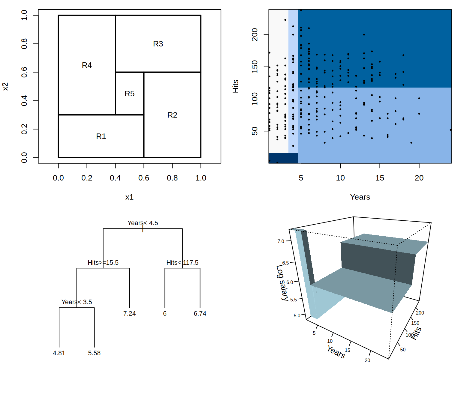
})Years and Hits.
from matplotlib.patches import Rectangle

hitters_tree_five = DecisionTreeRegressor(max_leaf_nodes=5, random_state=0)
hitters_tree_five.fit(X_hitters, y_hitters);
years_grid = np.linspace(1, 24, 120)
hits_grid = np.linspace(1, 238, 120)
yy, hh = np.meshgrid(years_grid, hits_grid)
grid = pd.DataFrame({"Years": yy.ravel(), "Hits": hh.ravel()})
pred_grid = hitters_tree_five.predict(grid).reshape(yy.shape)

fig = plt.figure(figsize=(9, 8));
ax = fig.add_subplot(2, 2, 1);
pinwheel = [(0, 0, 0.6, 0.3, "R1"), (0.6, 0, 1, 0.6, "R2"), (0.4, 0.6, 1, 1, "R3"),
            (0, 0.3, 0.4, 1, "R4"), (0.4, 0.3, 0.6, 0.6, "R5")]
for x0, y0, x1, y1, label in pinwheel:
    ax.add_patch(Rectangle((x0, y0), x1 - x0, y1 - y0, fill=False, linewidth=2));
    ax.text((x0 + x1) / 2, (y0 + y1) / 2, label, ha="center", va="center");
ax.set_aspect("equal");
ax.set_xlabel("x1");
ax.set_ylabel("x2");
ax = fig.add_subplot(2, 2, 2);
ax.pcolormesh(years_grid, hits_grid, pred_grid, cmap="Blues", shading="auto");
ax.scatter(hitters["Years"], hitters["Hits"], s=4, color="black");
ax.set_xlabel("Years");
ax.set_ylabel("Hits");
ax = fig.add_subplot(2, 2, 3);
plot_tree(hitters_tree_five, feature_names=["Years", "Hits"], precision=3, impurity=False, ax=ax, fontsize=6);
ax = fig.add_subplot(2, 2, 4, projection="3d");
ax.plot_surface(yy, hh, pred_grid, cmap="Blues");
ax.set_xlabel("Years");
ax.set_ylabel("Hits");
ax.set_zlabel("Log salary");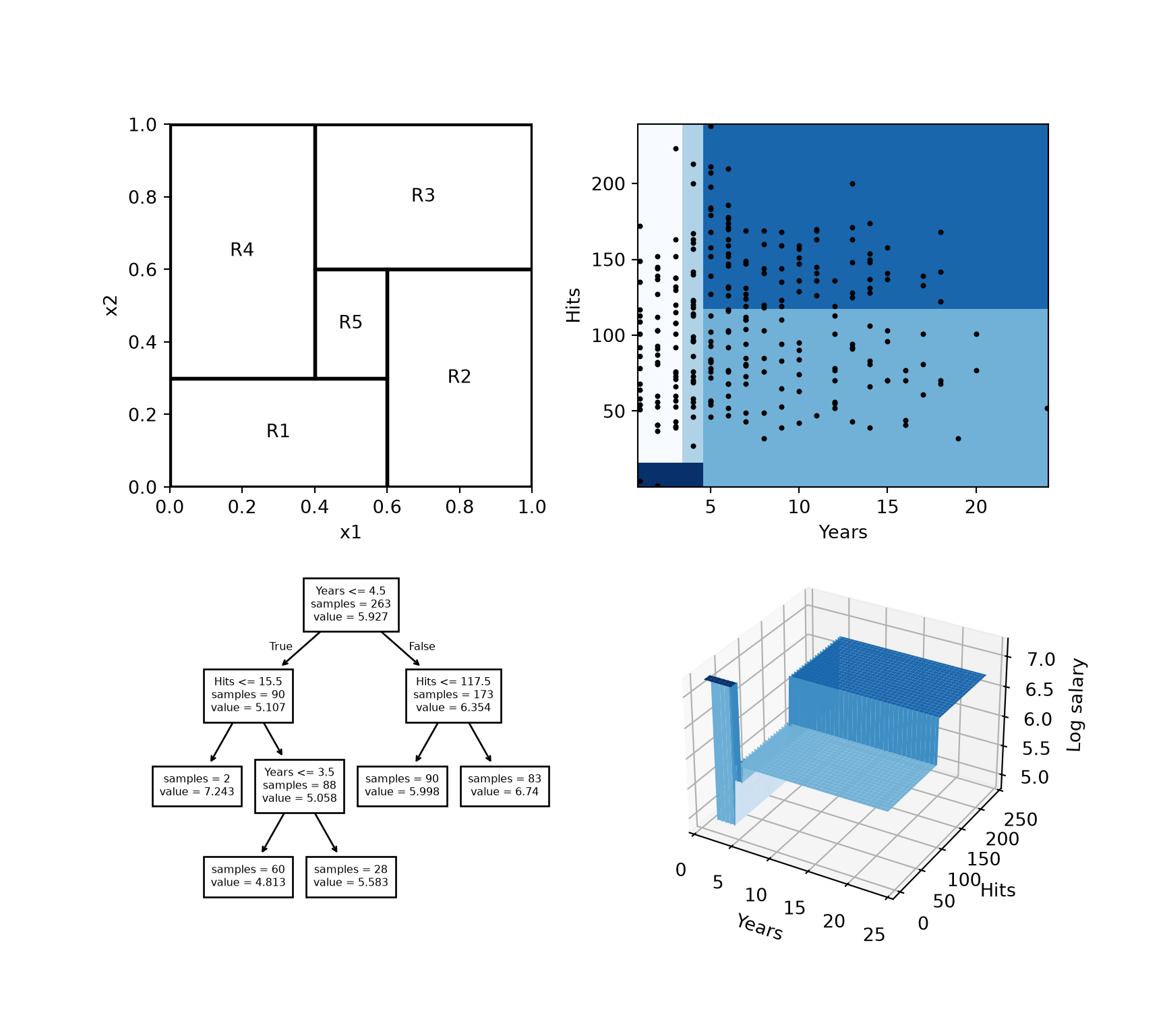
Starmer builds regression trees [14].
GeeksforGeeks fits a regression tree with scikit-learn [15].
Nothing so far says when to stop, and the greedy rule will not stop on its own. It can keep splitting until every leaf holds a single point, at which stage the training error is zero and the tree has memorized the data rather than learned from it.
Two conditions end the recursion naturally: every leaf is pure, so no split can gain anything; or no candidate split gains enough to justify the extra depth. The first is reachable on any dataset without contradictory labels, and reaching it is the failure mode rather than the goal.
So we limit the growth deliberately instead, with one or both of two simple controls:
a maximum depth, capping how many comparisons any prediction can involve
a minimum number of points required in a leaf, or required in a node before it may be split at all
Both say the same thing from opposite directions — do not create a region so small that the points inside it are as likely to be noise as signal — and both are hyperparameters, which we choose by the procedure of Model Selection rather than from the data. Both encode Occam’s razor, the principle that asks for the simplest hypothesis that fits the observations. For a tree, the simplest hypothesis is the smallest tree.
GeeksforGeeks explains pruning decision trees [16], including the depth and leaf-size limits above.
The two rules above stop the tree while it grows. The next two exercises ask whether stopping early can stop too soon.
Exercise 13 (Find the best first split when the label is an exclusive or) A label is the exclusive or of two binary features \(x_1\) and \(x_2\) when it is \(1\) exactly when \(x_1 \neq x_2\). Table 4 holds eight points labeled that way, two for each of the four combinations of feature values.
Compute the information gain of splitting the root on each of \(x_1\) and \(x_2\).
Choosing a split defines the information gain, and Measuring impurity defines the entropy \(H\) that it uses.
Exercise 14 (Look one split further) Continuing from Exercise 13, grow a tree on the eight points labeled by an exclusive or that splits the root on \(x_1\) anyway, and then splits each of the root’s two branches on \(x_2\).
Compare the number of training points that this four-leaf tree misclassifies with the number that the root alone misclassifies.
A leaf of a classification tree predicts the most common label among its training points, as in Decision trees.
Definition 2 (Cost-complexity pruning, weakest-link pruning) Let \(T_0\) be a tree grown on the training data to predict a numeric target, and let \(T\) be any tree obtained by collapsing some of the internal nodes of \(T_0\) into leaves. Write \(\card{T}\) for the number of leaves of \(T\), \(R_m\) for the region of its \(m\)th leaf, and \(\hy_{R_m}\) for the sample mean of the training targets in \(R_m\). Cost-complexity pruning, or weakest-link pruning, of \(T_0\) with penalty \(\regpar \geq 0\) replaces \(T_0\) by the tree \(T\) that minimizes the training squared error plus \(\regpar\) per leaf,
\[C_\regpar(T) = \sumto{m}{\card{T}} \sum_{i \,:\, \vx_i \in R_m} \devof{y_i}{\hy_{R_m}}^2 + \regpar \card{T}.\]
James et al. [17] and Hastie et al. [18] write the penalty as \(\alpha\); these notes write \(\regpar\), as for the penalties of Regularization.
Source: James et al. [17, Sec. 8.1.1].
Exercise 15 (Prune a tree whose middle subtree never wins) Consider a tree \(T_0\) that splits its root into an internal node \(C\) and a leaf \(D\), and splits \(C\) into leaves \(C_1\) and \(C_2\). Table 7 gives the training squared error of each leaf, and of the leaf that collapsing a node would leave in its place.
Find, for each penalty \(\regpar \geq 0\), the tree that cost-complexity pruning of \(T_0\) chooses.
List the trees that collapsing internal nodes of \(T_0\) gives, and compare their criteria \(C_\regpar\) as Example 4 does.
The trees that cost-complexity pruning chooses get smaller as the penalty grows, each inside the one before, so one pass over \(T_0\) finds them all. The chosen tree loses leaves as \(\regpar\) grows from \(0\), and each step collapses the internal node whose collapse raises the training squared error least per leaf removed, the weakest link that gives the method its second name [18, Sec. 9.2.2]. Solution 15 shows that a step can collapse more than one split at once.
The penalty \(\regpar\) is a hyperparameter, so we choose it by cross-validation and then prune the tree grown on all the training data with the chosen \(\regpar\) [17, Sec. 8.1.1], Algorithm 8.1. A classification tree is pruned the same way, with the training misclassification count, or a node impurity from Measuring impurity, in place of the training squared error; James et al. [17, Sec. 8.1.2] prefer the misclassification count when the goal is accurate prediction.
CART stands for Classification And Regression Trees.
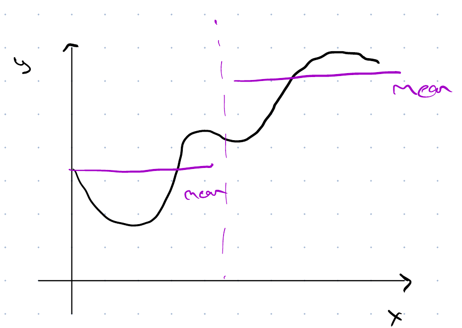
Handles discrete and continuous features.
Handles classification and regression with the same recursion, changing only the impurity measure.
Captures non-linear structure, because the regions are assembled by recursive cuts rather than described by one global function.
Overfits.
Does not need to store all the data, unlike KNN and kernel smoothing.
Fast.
Interpretable — but not really.
Subject to the curse of dimensionality.
The interpretability bullet needs explanation, because trees are usually promoted for it. A single fitted tree genuinely is as readable as a model gets: we can follow any prediction down the tree and report it as the few comparisons that produced it. The reservation concerns what that readability entitles you to conclude. A deep tree’s path is long enough that following it is no longer an explanation. The greedy rule commits to one split before considering what comes below, so a small change to the data can change an early split and alter everything under it. And two correlated features compete for the same split, so a feature’s absence from the tree is not evidence that it did not matter — only that the greedy rule chose its rival first.
Weinberger explains the curse of dimensionality [2], Lecture 4.
GeeksforGeeks explains:
James et al. [17], Chapter 8
Breiman et al. [8] — the book that introduced classification and regression trees
Zhou [21], Tree-Based Methods — slides on An Introduction to Statistical Learning, Chapter 8, with code in both R and Python
Starmer [22], on decision trees — an illustrated walk-through with little algebra
The Data Science Learning Community’s book clubs discuss An Introduction to Statistical Learning, Chapter 8, in recorded meetings: