Gaussian Processes

Published

Last modified: 2026-10-25

Show code
# The Python chunks on this page import numpy and pandas; reticulate provisions them.
library(reticulate)
py_require(c("numpy", "pandas"))

Written for these notes, following Rasmussen and Williams’ Gaussian Processes for Machine Learning [1] for the definitions, the regression formulas and the marginal likelihood.

1 From random weights to random functions

A model with random weights is a random function. This chapter takes that view to its limit: instead of a prior over the weights of a fixed model, put a prior directly on the function, and let the data update it.

ExrExercise 1 (Covariance of a random linear model)

Exercise 1 (Covariance of a random linear model) Suppose \(f(x) = \dprod{\vcoef}{\vfeatmap(x)}\) for a fixed feature map \(\vfeatmap\) and random weights \(\vcoef \dist \ndist{\vzero, I}\). For an input \(x\), find \(\E{f(x)}\).

Solution 1. Each \(f(x)\) is a linear combination of the Gaussian weights, so it is Gaussian with mean \(\E{f(x)} = \dprod{\E{\vcoef}}{\vfeatmap(x)} = 0\).

ExrExercise 2 (Covariance of a random linear model (part 2))

Exercise 2 (Covariance of a random linear model (part 2)) Use the setup of Exercise 1.

For two inputs \(x\) and \(z\), find \(\Covs{f(x)}{f(z)}\).

Solution 2. Because \(\E{\vcoef \tp{\vcoef}} = I\),

\[ \Covs{f(x)}{f(z)} = \E{\tp{\vfeatmap(x)}\, \vcoef \tp{\vcoef}\, \vfeatmap(z)} = \dprod{\vfeatmap(x)}{\vfeatmap(z)}. \]

This is the kernel \(K(x, z)\) of the kernel function definition in the SVM chapter: a random linear model in feature space is a random function whose covariances are kernel values. The same holds with infinitely many features, such as the RBF kernel’s.

DefDefinition 1 (Gaussian process)

Definition 1 (Gaussian process) A Gaussian process is a random function \(f: \reals^{\ninputvars} \to \reals\) for which every finite set of inputs \(x_1, \dots, x_n\) gives a jointly Gaussian vector \(\tp{(f(x_1), \dots, f(x_n))}\) [2].

DefDefinition 2 (Mean function)

Definition 2 (Mean function) The mean function of a Gaussian process \(f\) (Definition 1) is \(m(x) = \E{f(x)}\) [2].

DefDefinition 3 (Covariance function (kernel))

Definition 3 (Covariance function (kernel)) The covariance function (kernel) of a Gaussian process \(f\) (Definition 1) is \(k(x, z) = \Covs{f(x)}{f(z)}\) [3]. At inputs \(x_1, \dots, x_n\) it gives the matrix \(\matr{K}\) with \(\matr{K}_{ij} = k(x_i, x_j)\). The covariance function must be a valid kernel: every \(\matr{K}\) it produces must be symmetric and positive semi-definite [1, Ch. 4].

RemarkRemark 1 (Notation for a Gaussian process)

Remark 1 (Notation for a Gaussian process). A Gaussian process is determined by its mean function (Definition 2) \(m\) and covariance function (Definition 3) \(k\), and we write

\[ f \dist \operatorname{GP}(m, k). \]

At inputs \(x_1, \dots, x_n\) the vector of function values is \(\ndist{\vec{m}, \matr{K}}\), with \(\vec{m}_i = m(x_i)\) and \(\matr{K}_{ij} = k(x_i, x_j)\).

ExmExample 1 (The kernel matrix of five cars)

Example 1 (The kernel matrix of five cars) In the Auto data [4], standardize horsepower and take the first five cars. With the RBF covariance function \(k(x, z) = \expf{-(x - z)^2 / (2\bandwidth^2)}\) and length scale \(\bandwidth = 0.5\), a zero-mean Gaussian process gives their mpg values (standardized) the joint distribution \(\ndist{\vzero, \matr{K}}\):

import numpy as np
import pandas as pd

auto_gp = pd.read_csv("data/auto.csv").dropna(subset=["horsepower"])
hp_gp = auto_gp["horsepower"].to_numpy(float)
mpg_gp = auto_gp["mpg"].to_numpy(float)
# Standardize both variables, so a signal variance of 1 and a length scale
# in units of standard deviations are sensible defaults.
x_gp = (hp_gp - hp_gp.mean()) / hp_gp.std(ddof=1)
y_gp = (mpg_gp - mpg_gp.mean()) / mpg_gp.std(ddof=1)

def rbf_kernel(a, b, ell):
    # k(x, z) = exp(-(x - z)^2 / (2 ell^2)), for every pair from a and b.
    return np.exp(-(a[:, None] - b[None, :]) ** 2 / (2 * ell**2))

print(x_gp[:5].round(2))
[0.66 1.57 1.18 1.18 0.92]
print(rbf_kernel(x_gp[:5], x_gp[:5], 0.5).round(2))
[[1.   0.19 0.58 0.58 0.87]
 [0.19 1.   0.74 0.74 0.43]
 [0.58 0.74 1.   1.   0.87]
 [0.58 0.74 1.   1.   0.87]
 [0.87 0.43 0.87 0.87 1.  ]]
auto_gp <- na.omit(read.csv("data/auto.csv")[, c("mpg", "horsepower")])
# Standardize both variables, so a signal variance of 1 and a length scale
# in units of standard deviations are sensible defaults.
x_gp <- as.numeric(scale(auto_gp$horsepower))
y_gp <- as.numeric(scale(auto_gp$mpg))

rbf_kernel <- function(a, b, ell) {
  # k(x, z) = exp(-(x - z)^2 / (2 ell^2)), for every pair from a and b.
  exp(-outer(a, b, "-")^2 / (2 * ell^2))
}

round(x_gp[1:5], 2)
[1] 0.66 1.57 1.18 1.18 0.92
round(rbf_kernel(x_gp[1:5], x_gp[1:5], 0.5), 2)
     [,1] [,2] [,3] [,4] [,5]
[1,] 1.00 0.19 0.58 0.58 0.87
[2,] 0.19 1.00 0.74 0.74 0.43
[3,] 0.58 0.74 1.00 1.00 0.87
[4,] 0.58 0.74 1.00 1.00 0.87
[5,] 0.87 0.43 0.87 0.87 1.00

The diagonal is \(k(x, x) = 1\), the variance of each value. Cars 1 and 5 have standardized horsepower 0.66 and 0.92, so their values have correlation 0.87, while cars 1 and 2, at 0.66 and 1.57, have correlation 0.19: the process says that cars with similar horsepower have similar mpg, and the correlation falls toward 0 as the horsepower gap grows. Cars 3 and 4 have the same horsepower, so their correlation is 1.

The multivariate normal distribution is the finite-dimensional case. The remark on inner products in machine learning in the Mathematical Data Science notes mentions Gaussian processes among the methods built on kernels.

Show code
library(ggplot2)
set.seed(571)
grid_gp <- seq(-2, 3, length.out = 120)
draws_gp <- do.call(rbind, lapply(c(0.2, 0.5, 1.5), function(ell) {
  # A tiny jitter keeps the Cholesky factor numerically positive definite.
  gram <- rbf_kernel(grid_gp, grid_gp, ell) + 1e-8 * diag(length(grid_gp))
  # If z is standard normal and gram = L L', then L z has covariance gram.
  chol_lower <- t(chol(gram))
  f <- chol_lower %*% matrix(rnorm(length(grid_gp) * 5), ncol = 5)
  data.frame(
    x = rep(grid_gp, 5), f = as.vector(f), draw = rep(1:5, each = length(grid_gp)),
    ell = paste("length scale", ell, "SD of horsepower")
  )
}))
# The kernel works on z-scores of horsepower; the axis shows horsepower.
auto_hp <- na.omit(read.csv("data/auto.csv")$horsepower)
ggplot(draws_gp, aes(x * sd(auto_hp) + mean(auto_hp), f, group = draw)) +
  geom_line(colour = "grey35") +
  facet_wrap(~ell) +
  labs(x = "horsepower", y = "Function value, f(x)")
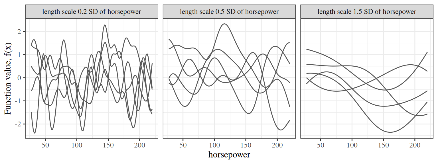
Figure 1: Five draws from a zero-mean Gaussian process prior with the RBF covariance function, for three length scales. Each draw is one random function, evaluated on a grid of horsepower values. The length scales are in units of the standard deviation of horsepower, because the kernel works on standardized horsepower, and the axis shows horsepower.
Three ggplot2 panels, one per length scale, each showing five smooth random curves over horsepower, from about 30 to 220. With a length scale of 0.2 standard deviations of horsepower the curves wiggle rapidly. With 0.5 they change slowly across the range. With 1.5 they are nearly flat curves with one gentle bend each.

The length scale \(\bandwidth\) sets how fast a draw can change; a longer one gives smoother functions.

ReadingRead

Görtler, Kehlbeck and Deussen give a visual exploration of Gaussian processes [5].

2 Prediction

ExrExercise 3 (Predicting one value from another)

Exercise 3 (Predicting one value from another) Suppose \(\tp{(f_1, y_1)}\) is jointly Gaussian with zero means, \(\Var{f_1} = 1\), \(\Var{y_1} = 1 + \tau^2\) and \(\Covs{f_1}{y_1} = c\). After observing \(y_1\), what is the mean of \(f_1\)?

TipHint

Write \(f_1 = a\, y_1 + e\) and choose \(a\) so that \(e\) is uncorrelated with \(y_1\). For jointly Gaussian variables, uncorrelated means independent.

Solution 3. Uncorrelated requires \(0 = \Covs{e}{y_1} = c - a(1 + \tau^2)\), so \(a = c / (1 + \tau^2)\). Since \(e\) is independent of \(y_1\), given \(y_1\) the value \(f_1 = a\, y_1 + e\) has

\[ \E{f_1 \mid y_1} = \frac{c}{1 + \tau^2}\, y_1. \]

The mean is linear in the observation.

ExrExercise 4 (Predicting one value from another (part 2))

Exercise 4 (Predicting one value from another (part 2)) Use the setup of Exercise 3.

After observing \(y_1\), what is the variance of \(f_1\)?

Solution 4. Since \(e\) is independent of \(y_1\), given \(y_1\) the value \(f_1 = a\, y_1 + e\) has

\[ \Var{f_1 \mid y_1} = \Var{e} = 1 - \frac{c^2}{1 + \tau^2}. \]

The variance does not depend on the observation: observing \(y_1\) can only shrink the uncertainty, by \(c^2 / (1 + \tau^2)\).

LemLemma 1 (Conditioning a scalar Gaussian)

Lemma 1 (Conditioning a scalar Gaussian) Suppose \(\tp{(f_1, y_1)}\) is jointly Gaussian with zero means, \(\Var{f_1} = 1\), \(\Var{y_1} = 1 + \tau^2\) and \(\Covs{f_1}{y_1} = c\) [6]. Then given \(y_1\),

\[ \E{f_1 \mid y_1} = \frac{c}{1 + \tau^2}\, y_1, \qquad \Var{f_1 \mid y_1} = 1 - \frac{c^2}{1 + \tau^2}. \]

Proof. By Solution 3 and Solution 4.

ExmExample 2 (Conditioning with \(c = 0.6\) and \(\tau = 0.5\))

Example 2 (Conditioning with \(c = 0.6\) and \(\tau = 0.5\)) Compare the formulas of Lemma 1 with the general Gaussian conditioning formula applied to the covariance matrix of \(\tp{(f_1, y_1)}\):

import numpy as np

c, tau = 0.6, 0.5
Sigma = np.array([[1.0, c], [c, 1 + tau**2]])
# General formula: slope = Cov(f, y) / Var(y); variance = Var(f) - Cov^2 / Var(y).
print(Sigma[0, 1] / Sigma[1, 1], c / (1 + tau**2))
0.48 0.48
print(Sigma[0, 0] - Sigma[0, 1] ** 2 / Sigma[1, 1], 1 - c**2 / (1 + tau**2))
0.712 0.712
c0 <- 0.6; tau <- 0.5
Sigma <- matrix(c(1, c0, c0, 1 + tau^2), 2)
# General formula: slope = Cov(f, y) / Var(y); variance = Var(f) - Cov^2 / Var(y).
c(Sigma[1, 2] / Sigma[2, 2], c0 / (1 + tau^2))
[1] 0.48 0.48
c(Sigma[1, 1] - Sigma[1, 2]^2 / Sigma[2, 2], 1 - c0^2 / (1 + tau^2))
[1] 0.712 0.712
LemTheorem 1 (Gaussian process regression)

Theorem 1 (Gaussian process regression) Let \(f \dist \operatorname{GP}(0, k)\), and observe \(y_i = f(x_i) + \noise_i\) with \(\noise_i \siid \ndist{0, \tau^2}\) for \(i = 1, \dots, n\). Write \(\matr{K}_{ij} = k(x_i, x_j)\) and \(\vec{k}_*(x) = \tp{(k(x, x_1), \dots, k(x, x_n))}\). Then given \(\vy\), the value \(f(x)\) at any input \(x\) is Gaussian with

\[ \begin{aligned} \mu_*(x) &= \tp{\vec{k}_*(x)}\, \inv{\matr{K} + \tau^2 I}\, \vy,\\ v_*(x) &= k(x, x) - \tp{\vec{k}_*(x)}\, \inv{\matr{K} + \tau^2 I}\, \vec{k}_*(x). \end{aligned} \]

Proof. The vector \(\tp{(f(x), \vy)}\) is jointly Gaussian with zero mean. Its blocks are \(\Var{f(x)} = k(x, x)\), \(\Covs{f(x)}{\vy} = \tp{\vec{k}_*(x)}\) and \(\Var{\vy} = \matr{K} + \tau^2 I\). Conditioning a Gaussian on a block, as in Lemma 1 with vectors in place of scalars [1], Appendix A.2, gives the stated mean and variance.

ExmExample 3 (Gaussian process regression on the Auto data)

Example 3 (Gaussian process regression on the Auto data) Continuing with the standardized horsepower and mpg of Example 1, compute Theorem 1’s \(\mu_*(x)\) and \(\sqrt{v_*(x)}\) on a grid of horsepower values, with the RBF covariance function, \(\bandwidth = 0.5\) and noise variance \(\tau^2 = 0.25\):

def gp_posterior(x, y, x_new, ell, noise_var):
    K = rbf_kernel(x, x, ell) + noise_var * np.eye(len(x))
    # Factor K = L L' once. Solving with L is cheaper and more stable than inverting K.
    L = np.linalg.cholesky(K)
    alpha = np.linalg.solve(L.T, np.linalg.solve(L, y))
    K_new = rbf_kernel(x_new, x, ell)
    mean = K_new @ alpha
    V = np.linalg.solve(L, K_new.T)
    # k(x, x) = 1 for the RBF kernel, so the variance is 1 minus what the data explain.
    var = 1 - np.sum(V**2, axis=0)
    return mean, var

grid_py = np.linspace(-2, 3, 6)
mean_py, var_py = gp_posterior(x_gp, y_gp, grid_py, 0.5, 0.25)
print(grid_py.round(1))
[-2. -1.  0.  1.  2.  3.]
print(mean_py.round(3))
[ 0.355  1.205 -0.353 -0.992 -1.249 -1.339]
print(np.sqrt(var_py).round(3))
[0.716 0.062 0.064 0.085 0.142 0.178]
gp_posterior <- function(x, y, x_new, ell, noise_var) {
  K <- rbf_kernel(x, x, ell) + noise_var * diag(length(x))
  # Factor K = L L' once. Solving with L is cheaper and more stable than inverting K.
  R <- chol(K)  # upper triangular, K = R'R
  alpha <- backsolve(R, forwardsolve(t(R), y))
  K_new <- rbf_kernel(x_new, x, ell)
  V <- forwardsolve(t(R), t(K_new))
  # k(x, x) = 1 for the RBF kernel, so the variance is 1 minus what the data explain.
  list(mean = drop(K_new %*% alpha), var = 1 - colSums(V^2))
}

grid_r <- seq(-2, 3, length.out = 6)
post_r <- gp_posterior(x_gp, y_gp, grid_r, 0.5, 0.25)
round(grid_r, 1)
[1] -2 -1  0  1  2  3
round(post_r$mean, 3)
[1]  0.355  1.205 -0.353 -0.992 -1.249 -1.339
round(sqrt(post_r$var), 3)
[1] 0.716 0.062 0.064 0.085 0.142 0.178

Where the data are dense, the predictive standard deviation is small: its smallest value on this grid is 0.06. The left end of the grid, standardized horsepower -2, is below every car in the data (the lowest is -1.52), so the standard deviation there is 0.72, about 12 times larger. The model reports its own uncertainty about where it has seen little data; a fitted line does not.

Show code
grid_fig <- seq(-1.7, 3.2, length.out = 200)
post_fig <- gp_posterior(x_gp, y_gp, grid_fig, 0.5, 0.25)
band_fig <- data.frame(
  x = grid_fig, mean = post_fig$mean,
  lower = post_fig$mean - 2 * sqrt(post_fig$var),
  upper = post_fig$mean + 2 * sqrt(post_fig$var)
)
# The fit uses z-scores; the axes show horsepower and mpg.
hp_mean <- mean(auto_gp$horsepower)
hp_sd <- sd(auto_gp$horsepower)
mpg_mean <- mean(auto_gp$mpg)
mpg_sd <- sd(auto_gp$mpg)
to_hp <- function(z) z * hp_sd + hp_mean
to_mpg <- function(z) z * mpg_sd + mpg_mean
ggplot() +
  geom_point(aes(to_hp(x_gp), to_mpg(y_gp)), alpha = 0.4) +
  geom_ribbon(aes(to_hp(x), ymin = to_mpg(lower), ymax = to_mpg(upper)),
              data = band_fig, alpha = 0.3) +
  geom_line(aes(to_hp(x), to_mpg(mean)), data = band_fig, linewidth = 1) +
  labs(x = "horsepower", y = "mpg")
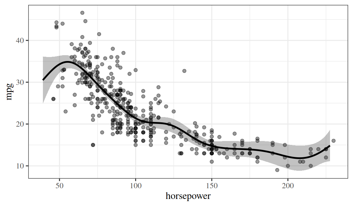
Figure 2: Gaussian process regression of mpg on horsepower in the Auto data, with the RBF covariance function, fitted to the standardized values and drawn on the original scales. The line is the posterior mean and the band is two posterior standard deviations of the function value.
A ggplot2 scatterplot of mpg, from about 10 to 45, against horsepower, from 46 to 230, for 392 cars, falling steeply and curving up toward the right. A smooth line follows the trend of the points, and a narrow grey band around it widens at both ends, where there are few cars.
ExrExercise 5 (The posterior mean as a kernel expansion)

Exercise 5 (The posterior mean as a kernel expansion) Write \(\vec{\alpha} = \inv{\matr{K} + \tau^2 I}\, \vy\). Express \(\mu_*(x)\) as a sum over the training inputs.

Solution 5. By Theorem 1,

\[ \mu_*(x) = \sum_{i=1}^n \alpha_i\, k(x, x_i). \]

ExrExercise 6 (The posterior mean as a kernel expansion (part 2))

Exercise 6 (The posterior mean as a kernel expansion (part 2)) Use the setup of Exercise 5.

What does this say about the form of the fitted function?

Solution 6. The fitted function is a weighted sum of one kernel bump centered at each training input.

ExrExercise 7 (The posterior mean as a kernel expansion (part 3))

Exercise 7 (The posterior mean as a kernel expansion (part 3)) Use the setup of Exercise 5.

Which method from earlier in the notes finds the same function?

Solution 7. This is the form that the representer theorem gives in Support Vector Machines, and it is the fit of kernel ridge regression: ridge regression with penalty \(\regpar = \tau^2\) in the feature space of the kernel. The fitted function \(\mu_*\) of the Gaussian process is the kernel ridge solution. What the Gaussian process adds is \(v_*(x)\), the uncertainty about the fit, which does not depend on \(\vy\) at all.

3 Choosing the covariance function

DefDefinition 4 (Hyperparameters)

Definition 4 (Hyperparameters) The covariance function’s (Definition 3) hyperparameters are such quantities as the length scale \(\bandwidth\) and the noise variance \(\tau^2\).

DefDefinition 5 (Marginal likelihood)

Definition 5 (Marginal likelihood) The marginal likelihood of the data under a Gaussian process is the density of \(\vy\) with the function values integrated out [7]. Since \(\vy \dist \ndist{\vzero, \matr{K} + \tau^2 I}\), its logarithm is

\[ \log p(\vy \mid X) = -\frac{1}{2}\, \tp{\vy} \inv{\matr{K} + \tau^2 I} \vy - \frac{1}{2} \log \detf{\matr{K} + \tau^2 I} - \frac{n}{2} \log\paren{2\pi}. \]

RemarkRemark 2 (Reading the marginal likelihood)

Remark 2 (Reading the marginal likelihood). In the log marginal likelihood, the first term rewards fitting the data and the second penalizes a model that is more flexible than it needs to be. The covariance function’s hyperparameters (Definition 4) are chosen by maximizing this quantity [1, Ch. 5], [7].

ExmExample 4 (Choosing the length scale on the Auto data)

Example 4 (Choosing the length scale on the Auto data) Evaluate the log marginal likelihood of Definition 5 for the Auto data on a grid of length scales \(\bandwidth\) and noise variances \(\tau^2\), and report the best pair:

def log_marginal_likelihood(x, y, ell, noise_var):
    K = rbf_kernel(x, x, ell) + noise_var * np.eye(len(x))
    L = np.linalg.cholesky(K)
    alpha = np.linalg.solve(L.T, np.linalg.solve(L, y))
    # log det K = 2 * sum(log diag(L)) for K = L L'.
    return -0.5 * y @ alpha - np.sum(np.log(np.diag(L))) - 0.5 * len(x) * np.log(2 * np.pi)

ells_py = [0.1, 0.2, 0.3, 0.5, 0.8, 1.2, 2.0]
noises_py = [0.05, 0.1, 0.2, 0.4, 0.8]
scores_py = {
    (ell, nv): log_marginal_likelihood(x_gp, y_gp, ell, nv)
    for ell in ells_py for nv in noises_py
}
best_py = max(scores_py, key=scores_py.get)
print(best_py, round(scores_py[best_py], 2))
(0.8, 0.4) -342.73
log_marginal_likelihood <- function(x, y, ell, noise_var) {
  K <- rbf_kernel(x, x, ell) + noise_var * diag(length(x))
  R <- chol(K)  # K = R'R
  alpha <- backsolve(R, forwardsolve(t(R), y))
  # log det K = 2 * sum(log diag(R)).
  -0.5 * sum(y * alpha) - sum(log(diag(R))) - 0.5 * length(x) * log(2 * pi)
}

ells_r <- c(0.1, 0.2, 0.3, 0.5, 0.8, 1.2, 2.0)
noises_r <- c(0.05, 0.1, 0.2, 0.4, 0.8)
grid_ml <- expand.grid(ell = ells_r, noise_var = noises_r)
grid_ml$score <- mapply(
  function(ell, nv) log_marginal_likelihood(x_gp, y_gp, ell, nv),
  grid_ml$ell, grid_ml$noise_var
)
best_ml <- grid_ml[which.max(grid_ml$score), ]
best_ml

The best pair on the grid is \(\bandwidth =\) 0.8 and \(\tau^2 =\) 0.4, with log marginal likelihood -342.7. The length scale \(\bandwidth = 0.5\) used in Example 3 scores -346.7 at its best noise variance, 4.0 log units lower than the best pair on this grid. The best noise variance estimates how much standardized mpg varies around the smooth trend.

The cost is the weak point of Gaussian processes: every prediction and every likelihood evaluation factors an \(n \times n\) matrix, which takes time proportional to \(n^3\), so exact Gaussian processes suit data sets of up to a few thousand rows. Approximations such as inducing points [1, Ch. 8] extend them further. The kernel also encodes the structure assumed: an RBF kernel gives very smooth functions, and sums and products of kernels combine trends, periodic effects and interactions.

4 Further reading

  • Rasmussen and Williams [1], the standard reference, free online

  • Hastie et al. [8], Section 5.8, on reproducing kernel Hilbert spaces

  • Stanford University [9], Stanford EE 278 (taught by Tsachy Weissman) — handwritten notes on MMSE estimation and conditional expectation, the geometry of MMSE estimation, and Gaussian conditioning with Gaussian MMSE estimation, which cover the conditioning step behind a GP posterior; the geometry of MMSE estimation is the orthogonal projection from linear algebra

References

[1]
C. E. Rasmussen and C. K. I. Williams, Gaussian processes for machine learning. MIT Press, 2006. Available: https://gaussianprocess.org/gpml/
[2]
Wikipedia contributors, “Gaussian process — Wikipedia, the free encyclopedia.” 2026. Available: https://en.wikipedia.org/wiki/Gaussian_process
[3]
Wikipedia contributors, “Covariance function — Wikipedia, the free encyclopedia.” 2026. Available: https://en.wikipedia.org/wiki/Covariance_function
[4]
G. James, D. Witten, T. Hastie, and R. Tibshirani, An introduction to statistical learning with applications in R, 2nd ed. Springer, 2021. Available: https://www.statlearning.com/
[5]
J. Görtler, R. Kehlbeck, and O. Deussen, “A visual exploration of Gaussian processes,” Distill, 2019, doi: 10.23915/distill.00017.
[6]
Wikipedia contributors, “Multivariate normal distribution — Wikipedia, the free encyclopedia.” 2026. Available: https://en.wikipedia.org/wiki/Multivariate_normal_distribution
[7]
Wikipedia contributors, “Marginal likelihood — Wikipedia, the free encyclopedia.” 2026. Available: https://en.wikipedia.org/wiki/Marginal_likelihood
[8]
T. Hastie, R. Tibshirani, and J. Friedman, The elements of statistical learning: Data mining, inference, and prediction, 2nd ed. Springer, 2009. Available: https://hastie.su.domains/ElemStatLearn/
[9]
Stanford University, “EE 278, probability and statistical inference: Fall 2024 lecture notes.” Handwritten lecture notes, Lectures 1–17, 2024. Available: http://web.stanford.edu/class/ee278/lectures.html
Back to top