Logistic Regression

# The Python chunks on this page import these packages; reticulate provisions them.
library(reticulate)
py_require(c("numpy", "pandas", "statsmodels", "scipy", "scikit-learn", "matplotlib"))

NoteSource

Adapted from Brian Hutchinson’s Fall 2025 lecture notes, reorganized as exercises. It also draws on Kameron Decker Harris’ 2022 weekly notes, for the log-odds view, the margin form of the loss and the hand-drawn figures, and on Logan Sizemore’s Spring 2025 lectures on classification and on multinomial logistic regression, for why thresholding a linear fit fails, where cross-entropy comes from, and the redundant weight vector.

Hutchinson’s version introduces gradient descent as a side topic partway through. That material now has a chapter of its own, so we keep the side topic as an outtake rather than repeat it here. Solution 103 corrects the spurious \(1/\nobs\) in the source’s multinomial gradient and flags the correction rather than fixing it silently.

1 Predicting a category

Linear regression predicts a number. A great many questions are not about a number: whether a patient recovers, whether an email is spam, which of ten digits a scan shows.

Let the data be \(\mathcal{X} = \set{(\vx_1, y_1), \ldots, (\vx_n, y_n)}\) with \(\vx_i \in \reals^{\ninputvars}\) and \(y_i\) a label rather than a measurement. Two labels is binary classification, which most of this chapter covers; more than two is multi-class classification, which Section 12 covers.

We could predict the label directly. Predicting \(P(Y = 1 \mid \vx)\) is more informative: whoever uses the prediction can decide how to act on it, because a probability states how confident the model is and a class label alone does not. A model of \(P(Y \mid \vx)\) is discriminative: it models the conditional distribution of the label given the features, without modelling the distribution of the features.

The simplest model of anything is a constant. The next simplest is built from a linear function, which is where this chapter starts.

VideosWatch

Hutchinson teaches classification and decision boundaries (6 min) [1]. The video site requires a login, which enrolled students find in the syllabus.

ExrExercise 1 (Fitting a line to a yes-or-no outcome)

Exercise 1 (Fitting a line to a yes-or-no outcome) The Western Collaborative Group Study followed 3154 middle-aged men for coronary heart disease [2]. In data/wcgs.csv, the column chd holds each man’s outcome \(y_i \in \{0, 1\}\): \(1\) if man \(i\) had an incident case and \(0\) if not. To predict chd, we try one feature: man \(i\)’s body mass index \(x_i\), from the column bmi. We do not know that bmi is related to chd. Later WCGS examples use age at enrollment (age) as the main covariate. This exercise uses bmi instead, to show what a straight line does to a yes-or-no outcome. The column dibpat records each man’s behavior pattern, type A or type B. This exercise pools the men of both patterns, so it ignores that column. We already know how to fit \(\hy = \dprod{\vcoef}{\vx}\) by least squares. Treat the two values of chd as the numbers \(0\) and \(1\), and fit linear regression in R or Python.

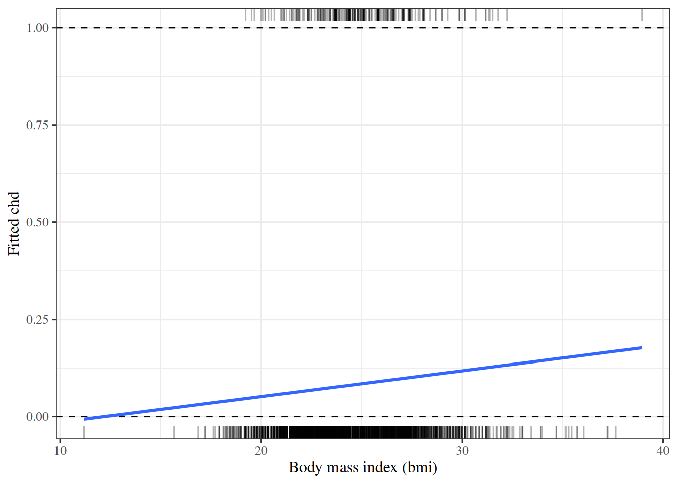
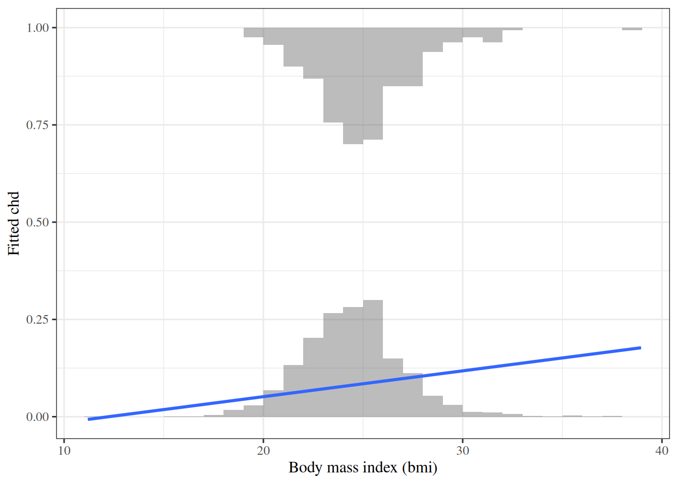
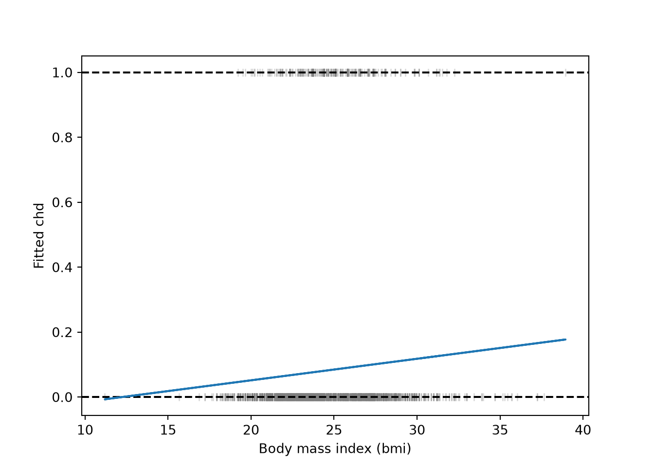
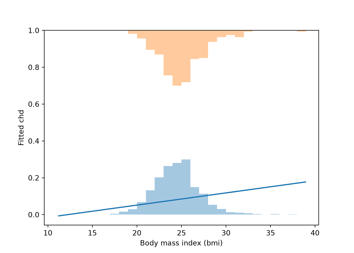
Fit a line of chd on bmi. Report its slope and intercept, the range of the fitted \(\hy\), and how many men have a fitted \(\hy\) outside \([0, 1]\). Then plot the data and the fitted line. Hint: because chd takes only the values \(0\) and \(1\), plotted points overlap at the two vertical coordinates \(y = 0\) and \(y = 1\). Instead, consider a rug, with one tick per man along the bottom edge for chd \(= 0\) and along the top edge for chd \(= 1\), and/or two histograms of bmi, one along the line \(y = 0\) for chd \(= 0\) and one extending downward from the line \(y = 1\) for chd \(= 1\).

SolutionSolution 1

Solution 1. Read the data and fit the line by least squares.

R

wcgs <- read.csv("data/wcgs.csv")
fit_bmi <- lm(chd ~ bmi, data = wcgs)
fitted_bmi <- fitted(fit_bmi)
outside <- sum(fitted_bmi < 0 | fitted_bmi > 1)
c(coef(fit_bmi), range(fitted_bmi), outside = outside)

 (Intercept)          bmi                                outside 
-0.081181996  0.006634395 -0.006943111  0.177227706  1.000000000 

library(ggplot2)
ggplot(wcgs, aes(bmi, chd)) +
  geom_rug(data = subset(wcgs, chd == 0), sides = "b", alpha = 0.3) +
  geom_rug(data = subset(wcgs, chd == 1), sides = "t", alpha = 0.3) +
  geom_hline(yintercept = c(0, 1), linetype = "dashed") +
  geom_smooth(method = "lm", formula = y ~ x, se = FALSE) +
  labs(x = "Body mass index (bmi)", y = "Fitted chd")

Fitted line of chd on bmi in the WCGS data, with a rug of the men with chd = 1 along the top and chd = 0 along the bottom.

breaks <- seq(floor(min(wcgs$bmi)), ceiling(max(wcgs$bmi)), by = 1)
bars <- function(chd_value) {
  counts <- hist(wcgs$bmi[wcgs$chd == chd_value], breaks = breaks, plot = FALSE)$counts
  data.frame(xmin = head(breaks, -1), xmax = tail(breaks, -1),
             height = 0.3 * counts / max(counts))
}
bars0 <- bars(0)
bars1 <- bars(1)
ggplot(wcgs, aes(bmi, chd)) +
  geom_rect(data = bars0, aes(xmin = xmin, xmax = xmax, ymin = 0, ymax = height),
            inherit.aes = FALSE, alpha = 0.4) +
  geom_rect(data = bars1, aes(xmin = xmin, xmax = xmax, ymin = 1 - height, ymax = 1),
            inherit.aes = FALSE, alpha = 0.4) +
  geom_smooth(method = "lm", formula = y ~ x, se = FALSE) +
  labs(x = "Body mass index (bmi)", y = "Fitted chd")

The same line, with a histogram of bmi for the men with chd = 0 standing on the line y = 0 and one for the men with chd = 1 hanging from the line y = 1. Each histogram is scaled so its tallest bar is 0.3 high.

Python

import numpy as np
import pandas as pd

wcgs = pd.read_csv("data/wcgs.csv")
slope, intercept = np.polyfit(wcgs["bmi"], wcgs["chd"], 1)
fitted_bmi = intercept + slope * wcgs["bmi"]
print(intercept, slope, fitted_bmi.min(), fitted_bmi.max(),
      ((fitted_bmi < 0) | (fitted_bmi > 1)).sum())

-0.08118199613838391 0.00663439543322767 -0.006943111240566277 0.17722770598583387 1

import matplotlib.pyplot as plt

fig, ax = plt.subplots()
for chd, side in [(0, 0.0), (1, 1.0)]:
    bmi_chd = wcgs.loc[wcgs["chd"] == chd, "bmi"]
    ax.plot(bmi_chd, [side] * len(bmi_chd), "|", color="gray", alpha=0.3);
ax.axhline(0, linestyle="--", color="black");
ax.axhline(1, linestyle="--", color="black");
ax.plot(wcgs["bmi"], fitted_bmi);
ax.set_xlabel("Body mass index (bmi)");
ax.set_ylabel("Fitted chd");
plt.show()

Fitted line of chd on bmi in the WCGS data, with a rug of the men with chd = 1 along the top and chd = 0 along the bottom.

breaks = np.arange(np.floor(wcgs["bmi"].min()), np.ceil(wcgs["bmi"].max()) + 1)

fig, ax = plt.subplots()
for chd, base, sign in [(0, 0.0, 1), (1, 1.0, -1)]:
    counts, _ = np.histogram(wcgs.loc[wcgs["chd"] == chd, "bmi"], bins=breaks)
    ax.bar(breaks[:-1], sign * 0.3 * counts / counts.max(), width=1,
           bottom=base, align="edge", alpha=0.4);
ax.plot(wcgs["bmi"], fitted_bmi);
ax.set_xlabel("Body mass index (bmi)");
ax.set_ylabel("Fitted chd");
plt.show()

The same line, with a histogram of bmi for the men with chd = 0 standing on the line y = 0 and one for the men with chd = 1 hanging from the line y = 1. Each histogram is scaled so its tallest bar is 0.3 high.

The fitted line is \(\hy =\) -0.081 \(+\) 0.0066 \(\times\) bmi. Its fitted values range from -0.007 to 0.177, so 1 of the 3154 men (the one with the lowest bmi) has a fitted value outside \([0, 1]\). A value outside \([0, 1]\) cannot be a valid probability. More generally, a nonconstant affine function of \(\vx\) is unbounded in both directions: here the fitted line exceeds \(1\) above a bmi of 163.

ExrExercise 2 (Squared error on probabilities)

Exercise 2 (Squared error on probabilities) A patient has \(\hy = 0.7\) and another has \(\hy = 0.9\). Under the squared-error loss, what does the difference of \(0.2\) imply about the two patients? State whether that implication is appropriate for probabilities.

SolutionSolution 2

Solution 2. Under squared-error loss, a difference of \(0.2\) between \(0.7\) and \(0.9\) is weighted identically to a difference of \(0.2\) between \(0.3\) and \(0.5\), because squared error treats equal differences in probability as equal regardless of where the probabilities are in \([0, 1]\). However, moving from probability \(0.7\) to \(0.9\) more than triples the odds (from \(7/3 \approx 2.33\) to \(9\)), whereas moving from \(0.3\) to \(0.5\) increases the odds by a factor of \(7/3\) (from \(3/7 \approx 0.43\) to \(1\)). Equal differences in probability do not correspond to equal multiplicative changes in odds.

ExrExercise 3 (A correctly classified point far from the others)

Exercise 3 (A correctly classified point far from the others) Suppose the data are one-dimensional and perfectly ordered: every point with \(x < 0\) has \(y = 0\), and every point with \(x > 0\) has \(y = 1\). Add a single new point far out at \(x = 100\), also with \(y = 1\), a point the model already classifies correctly. Say what happens to the least-squares fit, and why that change is undesirable when the prediction is correct.

SolutionSolution 3

Solution 3. Adding the outlying point tilts the least-squares line toward that point and shifts the decision boundary.

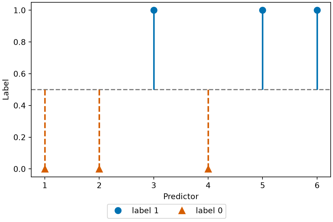
For the six points \(x = -3, -2, -1, 1, 2, 3\) with labels \(y = 0, 0, 0, 1, 1, 1\), least squares gives \(\hy =\) 0.5 \(+\) 0.2143\(\,x\), which classifies all six observations using the threshold \(\hy > 0.5\) without error.

Now add a seventh observation at \(x = 100\) with \(y = 1\) — an observation that the six-point line already places far on the \(y = 1\) side of the boundary. The least-squares line becomes \(\hy =\) 0.4903 \(+\) 0.005681\(\,x\). The slope decreases by a factor of about 38, and the six original fitted values are now between 0.473 and 0.507. At \(x = 1\), the fitted value is 0.4959 \(< 0.5\), so the observation at \(x = 1\) is misclassified as \(0\) even though its label is \(1\).

Adding an observation that is far on the correct side of the boundary causes the model to misclassify an observation it previously classified accurately.

This failure occurs because squared error penalizes \((\hy_i - y_i)^2\), and at \(x = 100\) the six-point line predicts \(\hy =\) 21.9, which contributes about 438 to the sum of squared residuals. Reducing the slope reduces that large squared residual at \(x = 100\) much more than it increases the squared residuals of the six points near the origin. Least squares therefore penalizes predictions that exceed \(1\) even when \(y_i = 1\), which distorts the classification boundary [3, Sec. 4.1.3].

ExrExercise 4 (Requirements for a classifier’s output)

Exercise 4 (Requirements for a classifier’s output) From Exercise 1, Exercise 2 and Exercise 3, state the two requirements that a classifier’s output should satisfy and that \(\dprod{\vcoef}{\vx}\) does not.

SolutionSolution 4

Solution 4. Two properties are required:

The output must be a valid probability. It must be in \([0, 1]\) for every \(\vx\) by construction, so that it can be interpreted as a class probability and combined with decision thresholds.

The loss must saturate on the side of the true label. Once an observation is classified accurately with high confidence, increasing its margin further should reduce the loss by almost nothing, so that points far on the correct side of the boundary do not distort the boundary near contested points.

The first requirement is satisfied by mapping the linear score into \((0,1)\) with the logistic sigmoid function (Exercise 7). The second requirement is satisfied by fitting the parameters by maximum Bernoulli likelihood (log loss) rather than least squares (Exercise 33). Both follow from modeling the log-odds as a linear function of \(\vx\) in Exercise 19.

ExrExercise 5 (Fitting the thresholded line)

Exercise 5 (Fitting the thresholded line) Check the first part of Solution 3 by computer, in Python, R or Julia.

Fit the least-squares line to the six points \(x = -3, -2, -1, 1, 2, 3\) with labels \(y = 0, 0, 0, 1, 1, 1\), and report its slope, its intercept, the input at which it crosses \(0.5\), and which of the six points the rule \(\hy > 0.5\) misclassifies.

Compute the slope and intercept directly from the least-squares formulas rather than calling a regression function.

SolutionSolution 5

Solution 5.

Python

x = [-3, -2, -1, 1, 2, 3]
y = [0, 0, 0, 1, 1, 1]

def fit(xs, ys):
    n = len(xs)
    xbar, ybar = sum(xs) / n, sum(ys) / n
    sxy = sum((xi - xbar) * (yi - ybar) for xi, yi in zip(xs, ys))
    sxx = sum((xi - xbar) ** 2 for xi in xs)
    m = sxy / sxx
    return m, ybar - m * xbar

def report(label, xs, ys):
    m, b = fit(xs, ys)
    cut = (0.5 - b) / m
    bad = [xi for xi, yi in zip(x, y) if (m * xi + b > 0.5) != (yi == 1)]
    print("%s slope %.6f  intercept %.4f  boundary %.2f  wrong: %s"
          % (label, m, b, cut, ", ".join(map(str, bad)) if bad else "none"))

report("without:", x, y)

without: slope 0.214286  intercept 0.5000  boundary 0.00  wrong: none

R

x <- c(-3, -2, -1, 1, 2, 3)
y <- c(0, 0, 0, 1, 1, 1)

fit <- function(xs, ys) {
  m <- sum((xs - mean(xs)) * (ys - mean(ys))) / sum((xs - mean(xs))^2)
  c(m, mean(ys) - m * mean(xs))
}

report <- function(label, xs, ys) {
  mb <- fit(xs, ys)
  cut <- (0.5 - mb[2]) / mb[1]
  bad <- x[(mb[1] * x + mb[2] > 0.5) != (y == 1)]
  cat(sprintf("%s slope %.6f  intercept %.4f  boundary %.2f  wrong: %s\n",
              label, mb[1], mb[2], cut,
              if (length(bad) == 0) "none" else paste(bad, collapse = ", ")))
}

report("without:", x, y)

without: slope 0.214286  intercept 0.5000  boundary 0.00  wrong: none

Julia

using Printf, Statistics

x = [-3, -2, -1, 1, 2, 3];
y = [0, 0, 0, 1, 1, 1];

function fit(xs, ys)
    m = sum((xs .- mean(xs)) .* (ys .- mean(ys))) / sum((xs .- mean(xs)) .^ 2)
    (m, mean(ys) - m * mean(xs))
end;

function report(label, xs, ys)
    m, b = fit(xs, ys)
    cut = (0.5 - b) / m
    bad = x[(m .* x .+ b .> 0.5) .!= (y .== 1)]
    @printf("%s slope %.6f  intercept %.4f  boundary %.2f  wrong: %s\n",
            label, m, b, cut, isempty(bad) ? "none" : join(bad, ", "))
end;

report("without:", x, y)

without: slope 0.214286  intercept 0.5000  boundary 0.00  wrong: none

without <- fit(x, y)
cut_without <- (0.5 - without[2]) / without[1]

The fit crosses \(0.5\) at \(x = 0\), midway between the classes, and classifies all six points correctly.

ExrExercise 6 (Watching an extreme point move the thresholded line)

Exercise 6 (Watching an extreme point move the thresholded line) Check the second part of Solution 3 by computer, in Python, R or Julia, using the six points of Exercise 5.

Refit with the seventh point \(x = 100\), \(y = 1\) added, and report the same four quantities, still evaluating classification accuracy on the original six points.

Compute the slope and intercept directly from the least-squares formulas rather than calling a regression function.

SolutionSolution 6

Solution 6. The code reuses x, y, fit and report from Solution 5.

Python

report("with   :", x + [100], y + [1])

with   : slope 0.005681  intercept 0.4903  boundary 1.71  wrong: 1

R

report("with   :", c(x, 100), c(y, 1))

with   : slope 0.005681  intercept 0.4903  boundary 1.71  wrong: 1

Julia

report("with   :", [x; 100], [y; 1])

with   : slope 0.005681  intercept 0.4903  boundary 1.71  wrong: 1

with_far <- fit(c(x, 100), c(y, 1))
cut_with <- (0.5 - with_far[2]) / with_far[1]
flipped <- x[(with_far[1] * x + with_far[2] > 0.5) != (y == 1)]

The second fit crosses \(0.5\) at \(x \approx 1.71\), past the class-\(1\) point at \(x = 1\), which it now classifies as class \(0\). Adding a point that the classifier already classified correctly causes it to misclassify a different point.

Although this example is one-dimensional and uses a small sample, neither property is essential. The same vulnerability to extreme points applies to every coefficient of a multi-feature least-squares fit, and the further the point is from the boundary, the larger its influence.

2 From a line to a probability

To keep the predictions in \([0, 1]\), we apply the logistic function

\[\sigmoid(\logodds) = \frac{1}{1 + e^{-\logodds}} \in (0, 1),\]

to \(\dprod{\vcoef}{\vx}\), which ranges over the whole real line. Setting the probability that the label is \(1\) to the result gives a logistic regression model.

The curve is also called a sigmoid, for its S-shape.

library(ggplot2)

sigmoid_df <- data.frame(eta = seq(-6, 6, length.out = 241))
sigmoid_df$p <- plogis(sigmoid_df$eta)
midpoint <- data.frame(eta = 0, p = plogis(0))

ggplot(sigmoid_df) +
  aes(eta, p) +
  geom_hline(yintercept = c(0, 1), linetype = "dotted", colour = "grey50") +
  geom_line(linewidth = 0.9, colour = "#0072B2") +
  geom_point(
    data = midpoint, shape = 21, size = 3, stroke = 1,
    fill = "#D55E00", colour = "black"
  ) +
  labs(x = "Log-odds η", y = "P(Y = 1)")

import matplotlib.pyplot as plt
import numpy as np
from scipy.special import expit

f_grid = np.linspace(-6, 6, 241)

fig, ax = plt.subplots(figsize=(5.5, 3.2), layout="constrained")
ax.axhline(0, color="grey", linestyle=":");
ax.axhline(1, color="grey", linestyle=":");
ax.plot(f_grid, expit(f_grid), color="#0072B2", linewidth=2);
ax.plot(0, expit(0), "o", markerfacecolor="#D55E00", markeredgecolor="black",
        markersize=8);
ax.set_xlabel("Log-odds η");
ax.set_ylabel("P(Y = 1)");
plt.show()

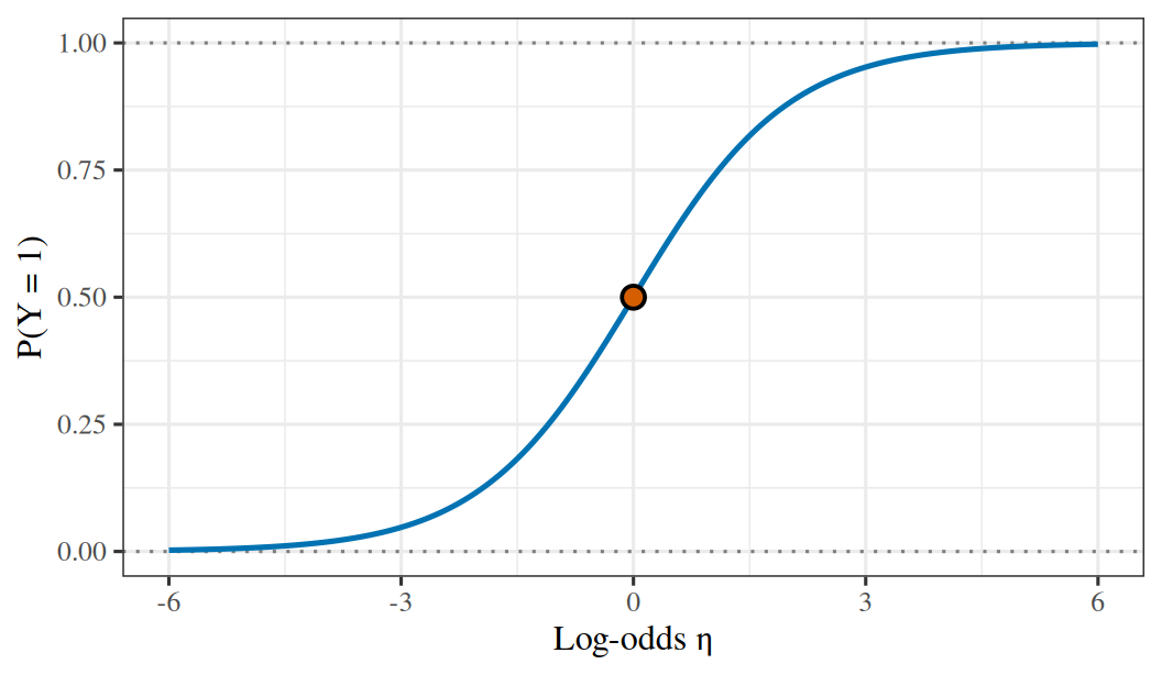
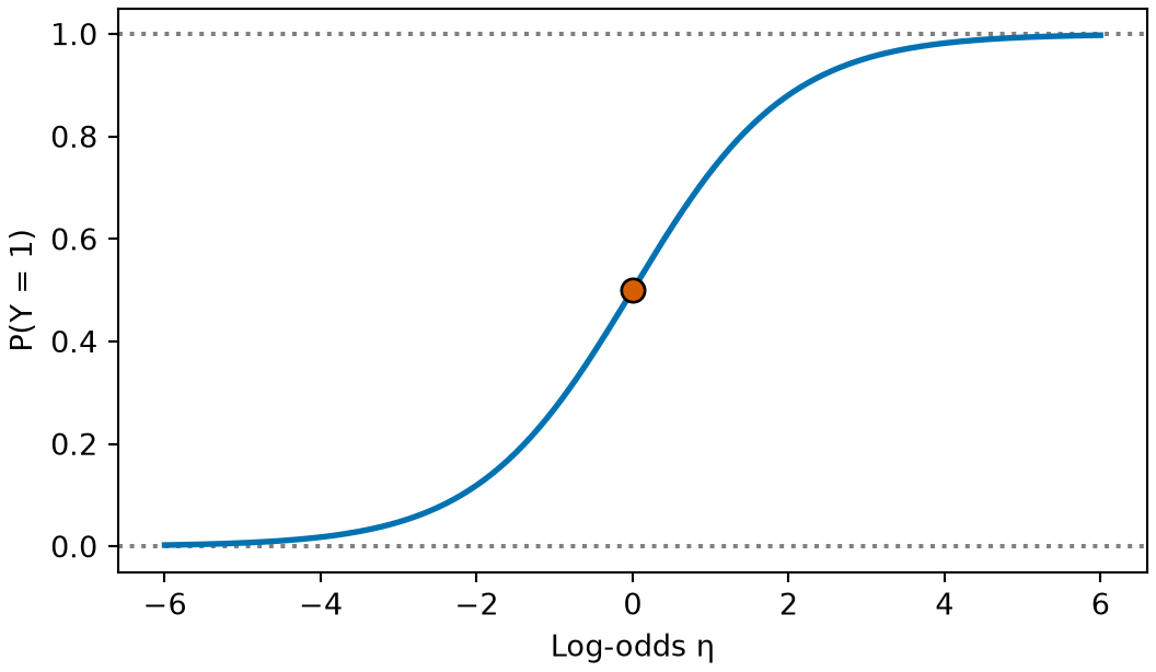
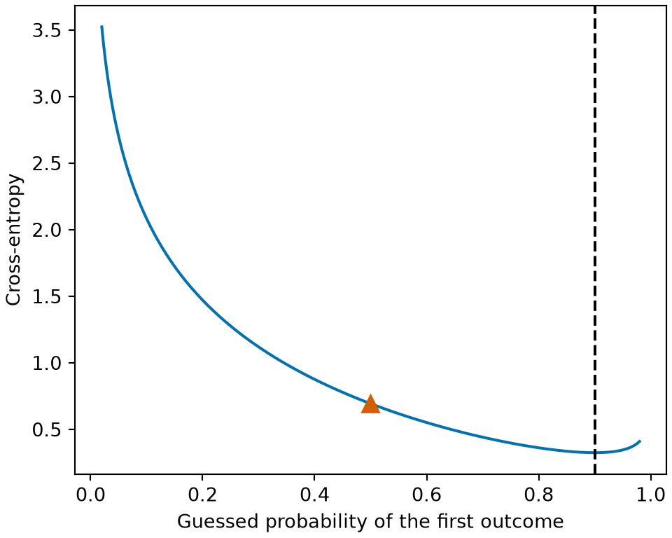
Figure 1: The logistic function, drawn over a log-odds axis labelled \(\logodds\). It passes through \(1/2\) at \(\logodds = 0\) and approaches \(0\) and \(1\) without reaching either.

R

(a)

Python

(b)

DefDefinition 1 (Logistic regression)

Definition 1 (Logistic regression) For a binary label \(\Outvar \in \set{0, 1}\) and feature vector \(\vpredvar\), a logistic regression model sets the probability that the label is \(1\) to the logistic function of a linear score with coefficient vector \(\vcoef\):

\[ \Prf{\Outvar = 1 \mid \vpredvar} = \sigmoidf{\dprod{\vcoef}{\vpredvar}}. \]

It is a linear regression model whose output passes through the logistic function.

ExmExample 1 (Logistic regression of coronary heart disease on age at enrollment, stratified by behavior pattern)

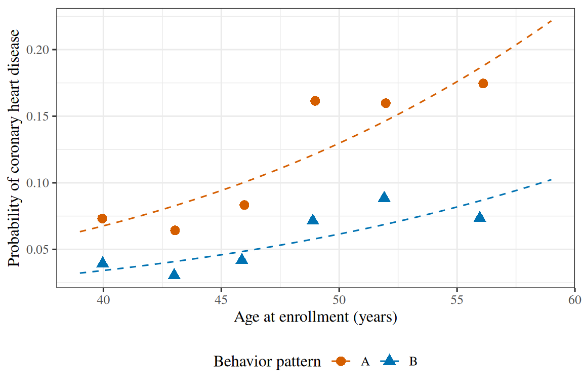
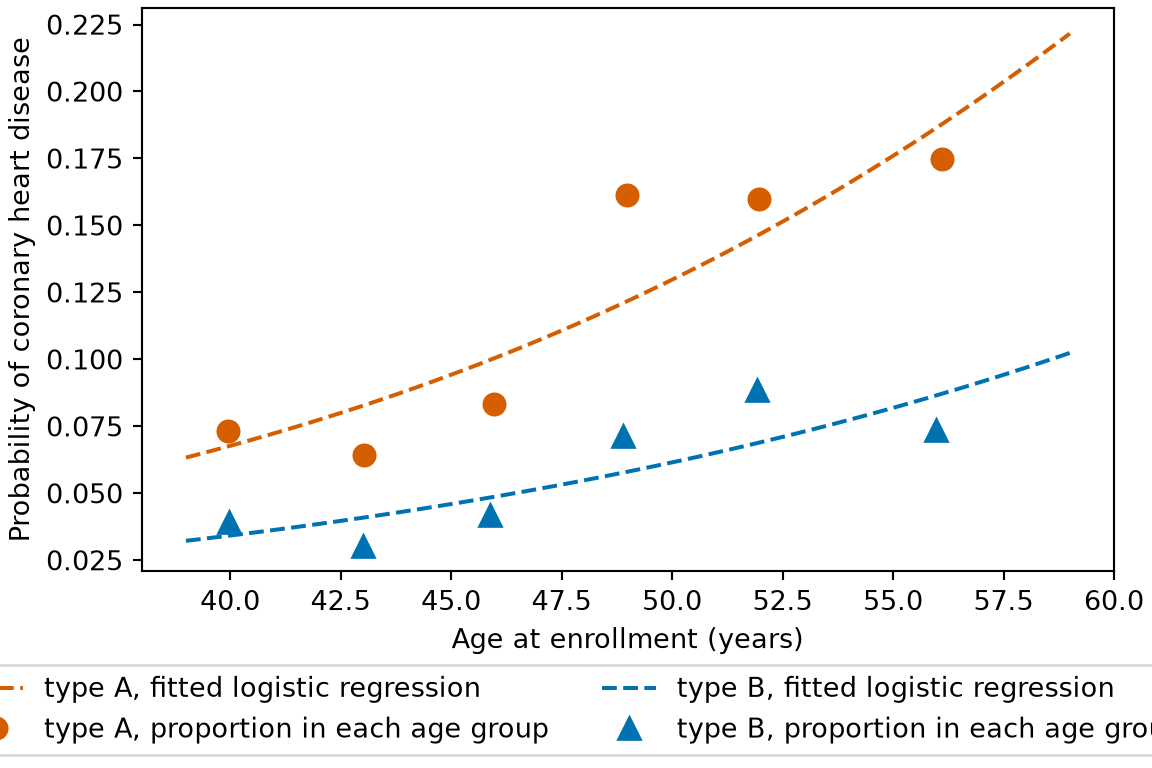
Example 1 (Logistic regression of coronary heart disease on age at enrollment, stratified by behavior pattern) In the WCGS data (data/wcgs.csv), the column dibpat records each man’s behavior pattern, type A or type B. The two patterns have different rates of coronary heart disease (chd), so we stratify: we fit a separate logistic regression of chd on age at enrollment (age) within each pattern, rather than combining the men. Each fit gives the fitted probability of disease at each age for its pattern:

wcgs_exm <- read.csv("data/wcgs.csv")
wcgs_fits <- lapply(
  split(wcgs_exm, wcgs_exm$dibpat),
  function(d) glm(chd ~ age, family = binomial, data = d)
)
exm_ages <- data.frame(age = c(40, 45, 50, 55))
cbind(
  exm_ages,
  sapply(wcgs_fits, predict, newdata = exm_ages, type = "response")
)

In both strata the fitted probability rises with age at enrollment, and it stays between \(0\) and \(1\) at every age. At every age shown, type A has the higher fitted probability.

library(ggplot2)
lrf_bins <- cut(wcgs_exm$age, breaks = c(38, 41, 44, 47, 50, 53, 59))
lrf_points <- aggregate(
  cbind(age, chd) ~ lrf_bins + dibpat, data = wcgs_exm, FUN = mean
)
lrf_curve <- do.call(rbind, lapply(names(wcgs_fits), function(type) {
  d <- data.frame(age = seq(min(wcgs_exm$age), max(wcgs_exm$age), length.out = 100))
  d$prob <- predict(wcgs_fits[[type]], newdata = d, type = "response")
  d$dibpat <- type
  d
}))
ggplot(lrf_curve, aes(age, prob, colour = dibpat)) +
  geom_line(linetype = "dashed") +
  geom_point(data = lrf_points, aes(y = chd, shape = dibpat), size = 3) +
  scale_colour_manual(values = c(A = "#D55E00", B = "#0072B2")) +
  labs(x = "Age at enrollment (years)", y = "Probability of coronary heart disease",
       colour = "Behavior pattern", shape = "Behavior pattern")

import matplotlib.pyplot as plt

points_lrf = r.lrf_points
curve_lrf = r.lrf_curve
fig, ax = plt.subplots(figsize=(6, 4), layout="constrained")
for pattern, colour, marker in [("A", "#D55E00", "o"), ("B", "#0072B2", "^")]:
    curve = curve_lrf[curve_lrf["dibpat"] == pattern]
    points = points_lrf[points_lrf["dibpat"] == pattern]
    ax.plot(curve["age"], curve["prob"], color=colour, linestyle="--",
            label=f"type {pattern}, fitted logistic regression");
    ax.plot(points["age"], points["chd"], color=colour, marker=marker, markersize=8,
            linestyle="", label=f"type {pattern}, proportion in each age group");
ax.set_xlabel("Age at enrollment (years)");
ax.set_ylabel("Probability of coronary heart disease");
fig.legend(loc="outside lower center", ncol=2);
plt.show()

Figure 2: The fitted probabilities of Example 1 (dashed curves), with the proportion of men who had coronary heart disease in each age group (circles for type A, triangles for type B). The groups are ages 39 to 41, 42 to 44, 45 to 47, 48 to 50, 51 to 53 and 54 to 59. Both curves rise with age at enrollment, type A lies above type B at every age, and each curve stays between \(0\) and \(1\).

R

(a)

Python

(b)

We separate two questions. The next two exercises ask whether this particular curve is a reasonable choice. Exercise 19 asks why it is the inevitable choice, rather than one S-shaped curve among many.

ExrExercise 7 (What the logistic function does)

Exercise 7 (What the logistic function does) \(\sigmoid(\logodds) = \dfrac{1}{1 + e^{-\logodds}}\). Establish its properties directly, because every one of them is used later.

Evaluate \(\sigmoid(0)\), and find \(\lim_{\logodds\to\infty}\sigmoid(\logodds)\) and \(\lim_{\logodds\to-\infty}\sigmoid(\logodds)\).

SolutionSolution 7

Solution 7. \[ \begin{aligned} \sigmoid(0) &= 1/(1 + e^{0}) \\ &= 1/2. \end{aligned} \]

As \(\logodds \to \infty\), \(e^{-\logodds} \to 0\), so \(\sigmoid(\logodds) \to 1\). As \(\logodds \to -\infty\), \(e^{-\logodds} \to \infty\), so \(\sigmoid(\logodds) \to 0\).

It is strictly increasing — Solution 9 gives a derivative that is positive everywhere — so \(\sigmoid\) is a bijection from \((-\infty,\infty)\) onto \((0,1)\), which is what Exercise 19 needed. The interval is open: \(\sigmoid\) never reaches \(0\) or \(1\), so the model is never completely certain.

ExrExercise 8 (What the logistic function does (part 2))

Exercise 8 (What the logistic function does (part 2)) Use the setup of Exercise 7.

Show that \(\sigmoid(-\logodds) = 1 - \sigmoid(\logodds)\). Say what this says about the model’s treatment of the two classes.

SolutionSolution 8

Solution 8. \[ \begin{aligned} \sigmoid(-\logodds) &= \frac{1}{1 + e^{\logodds}} \\ &= \frac{e^{-\logodds}}{e^{-\logodds}\paren{1 + e^{\logodds}}} \\ &= \frac{e^{-\logodds}}{e^{-\logodds} + 1} \\ &= \frac{1 + e^{-\logodds} - 1}{1 + e^{-\logodds}} \\ &= 1 - \sigmoid(\logodds) \end{aligned} \]

This says the model is symmetric in the two classes. Since

\[ \begin{aligned} \Pr[Y = 0 \mid \vx] &= 1 - \sigmoid(\dprod{\vcoef}{\vx}) \\ &= \sigmoid(-\dprod{\vcoef}{\vx}), \end{aligned} \]

fitting the model to the relabelled data \(\outvar \mapsto 1 - \outvar\) returns exactly \(-\vcoef\) and the same fitted probabilities. Which class you call \(1\) is a matter of labeling, not of modelling.

ExrExercise 9 (What the logistic function does (part 3))

Exercise 9 (What the logistic function does (part 3)) Use the setup of Exercise 7.

Show that \(\sigmoid'(\logodds) = \sigmoid(\logodds)\paren{1 - \sigmoid(\logodds)}\).

SolutionSolution 9

Solution 9. Expressing \(\sigmoid(\logodds)\) as \((1 + e^{-\logodds})^{-1}\) and applying the chain rule gives

\[ \begin{aligned} \sigmoid'(\logodds) &= -(1 + e^{-\logodds})^{-2} \cdot \frac{d}{d\logodds}\paren{1 + e^{-\logodds}} \\ &= -(1 + e^{-\logodds})^{-2} \cdot \paren{-e^{-\logodds}} \\ &= \frac{e^{-\logodds}}{\paren{1 + e^{-\logodds}}^{2}} \end{aligned} \]

Rewriting the numerator as \(e^{-\logodds} = \paren{1 + e^{-\logodds}} - 1\) and splitting the fraction gives

\[ \begin{aligned} \sigmoid'(\logodds) &= \frac{\paren{1 + e^{-\logodds}} - 1}{\paren{1 + e^{-\logodds}}^{2}} \\ &= \frac{1}{1 + e^{-\logodds}} - \frac{1}{\paren{1 + e^{-\logodds}}^{2}} \\ &= \sigmoid(\logodds) - \sigmoid(\logodds)^{2} \\ &= \sigmoid(\logodds)\paren{1 - \sigmoid(\logodds)} \end{aligned} \]

This identity simplifies the gradient of logistic regression in Exercise 48: the derivative of the model is expressed directly in terms of the model’s output \(\sigmoid(\logodds)\).

ExrExercise 10 (What the logistic function does (part 4))

Exercise 10 (What the logistic function does (part 4)) Use the setup of Exercise 7.

Where is \(\sigmoid'\) largest, and what is its value there? Give \(\sigmoid'(4)\) to three significant figures, and say what the comparison implies for a point the model already classifies confidently.

SolutionSolution 10

Solution 10. The derivative \(\sigmoid'= \sigmoid(1-\sigmoid)\) is a downward-opening parabola in \(\sigmoid\), maximized at \(\sigmoid = 1/2\), which corresponds to \(\logodds = 0\). Its maximum value is \(1/4\).

At \(\logodds = 4\), \(\sigmoid(4) = 0.98201\), so

\[ \begin{aligned} \sigmoid'(4) &= 0.98201 \times 0.01799 \\ &= 0.0177 \end{aligned} \]

to three significant figures, which is about \(1/14\) of the maximum. A point with large \(|\logodds|\) therefore is in a nearly flat region of \(\sigmoid\): a small change in \(\vcoef\) changes that point’s predicted probability by very little.

For a point that is confidently correct, this flatness provides the saturation that Exercise 4 required and that a linear model lacks. Because \(\sigmoid(\logodds)\) is already close to the true label, its residual is near zero and it contributes almost nothing to the gradient with respect to \(\vcoef\), so a point with a large positive margin does not outweigh contested points near the boundary.

For a point that is confidently wrong, the flatness of \(\sigmoid\) makes squared-error loss applied to \(\sigmoid(\dprod{\vcoef}{\vx})\) stall during optimization, because the \(\sigmoid'\) factor in the gradient of squared error shrinks when the prediction is furthest from the label. Exercise 48 shows that the log loss of Exercise 31 cancels the \(\sigmoid'\) factor, so a confidently wrong point contributes a gradient of magnitude close to \(\|\vx_i\|\). Log loss preserves saturation for confidently correct predictions while removing it for confidently wrong predictions.

ExrExercise 11 (What the logistic function does (part 5))

Exercise 11 (What the logistic function does (part 5)) Use the setup of Exercise 7.

There is a second sigmoid in common use, \(\tanh(\logodds) = \dfrac{\e{\logodds} - \e{-\logodds}}{\e{\logodds} + \e{-\logodds}}\). Prove \(\sigmoid(\logodds) = \tfrac{1}{2}\paren{1 + \tanh(\logodds/2)}\).

SolutionSolution 11

Solution 11. Starting from the right-hand side, write \(\tanh(\logodds/2)\) in exponentials and multiply numerator and denominator by \(e^{\logodds/2}\):

\[ \begin{aligned} \tanh(\logodds/2) &= \frac{e^{\logodds/2} - e^{-\logodds/2}}{e^{\logodds/2} + e^{-\logodds/2}} \\ &= \frac{e^{\logodds} - 1}{e^{\logodds} + 1} \end{aligned} \]

Then add \(1\), halve, and simplify:

\[ \begin{aligned} \tfrac{1}{2}\paren{1 + \tanh(\logodds/2)} &= \frac{1}{2} \cdot \frac{\paren{e^{\logodds} + 1} + \paren{e^{\logodds} - 1}}{e^{\logodds} + 1} \\ &= \frac{e^{\logodds}}{e^{\logodds} + 1} \\ &= \frac{1}{1 + e^{-\logodds}} \\ &= \sigmoid(\logodds) \end{aligned} \]

Thus the two sigmoid functions are related by a rescaling of the input and an affine transformation of the output. The function \(\tanh\) has range \((-1, 1)\), which matches the \(y \in \{+1, -1\}\) coding of Exercise 34 and is often used in hidden layers of neural networks where a zero-centered output is convenient. The logistic function \(\sigmoid\) has range \((0,1)\), which matches probabilities.

The logistic function, also called the sigmoid, is defined in the math prerequisites.

ExmExample 2 (Values of the logistic function in the WCGS data)

Example 2 (Values of the logistic function in the WCGS data) Fit the logistic model of chd on bmi to the WCGS data of Exercise 1, with \(\prob(\predvar) = \sigmoidf{\coef{0} + \coef{1}\,\predvar}\).

wcgs_logit <- glm(chd ~ bmi, family = binomial, data = wcgs)
coef(wcgs_logit)

(Intercept)         bmi 
-4.50856101  0.08427102 

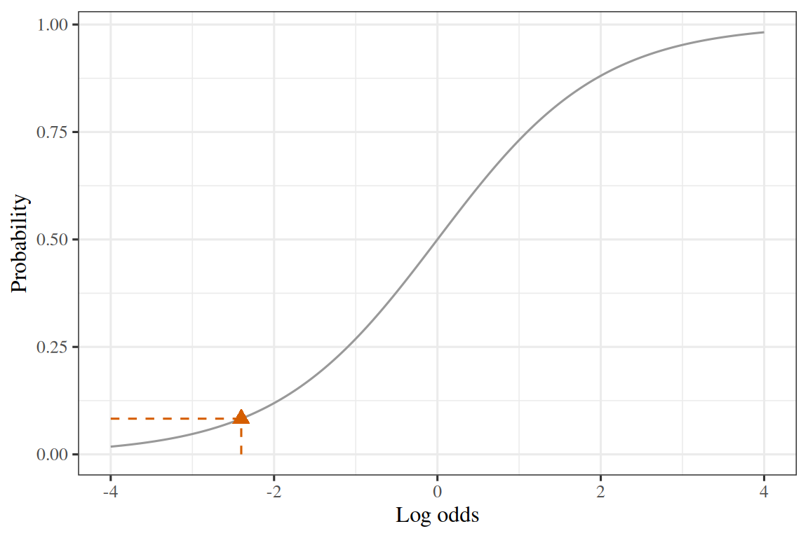
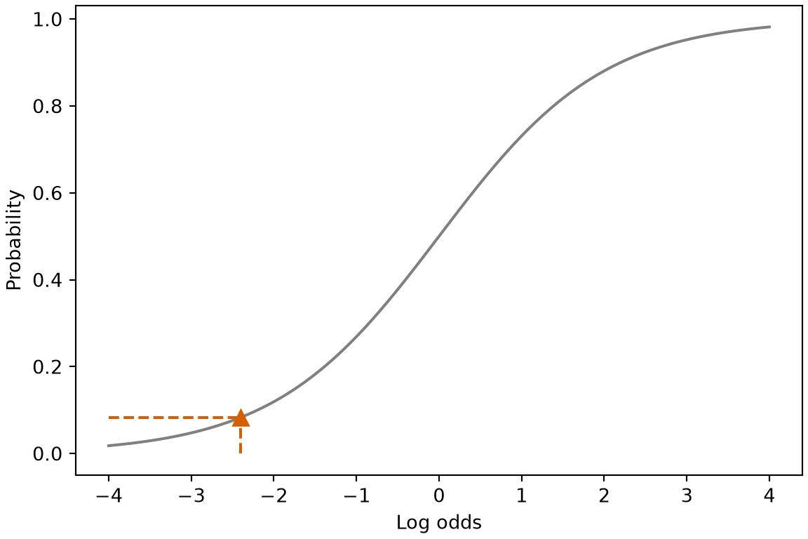
For a man with \(\text{bmi} = 25\), the linear score is \(\dprod{\vcoef}{\vpredvar} = -2.402\), and the logistic function maps it to \(\sigmoidf{-2.402} = 0.083\). The model therefore gives about a 8.3% probability that a man with a body mass index of 25 has an incident case of coronary heart disease.

library(ggplot2)
lfv_curve <- data.frame(z = seq(-6, 6, length.out = 241))
lfv_curve$p <- plogis(lfv_curve$z)
lfv_pts <- data.frame(z = c(-2, 0, 2))
lfv_pts$p <- plogis(lfv_pts$z)
lfv_pts$kind <- ifelse(lfv_pts$z == 0, "η = 0", "η = -2 and 2")
ggplot(lfv_curve, aes(z, p)) +
  geom_line(colour = "#0072B2") +
  geom_point(data = lfv_pts, aes(colour = kind, shape = kind), size = 3) +
  geom_text(data = lfv_pts, aes(label = round(p, 3)), hjust = -0.3, vjust = 1.2) +
  scale_colour_manual(values = c("η = 0" = "#0072B2", "η = -2 and 2" = "#D55E00")) +
  scale_shape_manual(values = c("η = 0" = 16, "η = -2 and 2" = 17)) +
  labs(x = "Log-odds η", y = "Logistic function of η", colour = NULL, shape = NULL)

import matplotlib.pyplot as plt
import numpy as np
from scipy.special import expit

grid_lfv = np.linspace(-6, 6, 241)
fig, ax = plt.subplots(figsize=(6, 4), layout="constrained")
ax.plot(grid_lfv, expit(grid_lfv), color="#0072B2");
for z_lfv, colour, marker in [(-2, "#D55E00", "^"), (0, "#0072B2", "o"), (2, "#D55E00", "^")]:
    ax.plot(z_lfv, expit(z_lfv), color=colour, marker=marker, markersize=8, linestyle="");
    ax.annotate(f"{expit(z_lfv):.3f}", (z_lfv, expit(z_lfv)), xytext=(8, -14),
                textcoords="offset points");
ax.set_xlabel("Log-odds η");
ax.set_ylabel("Logistic function of η");
plt.show()

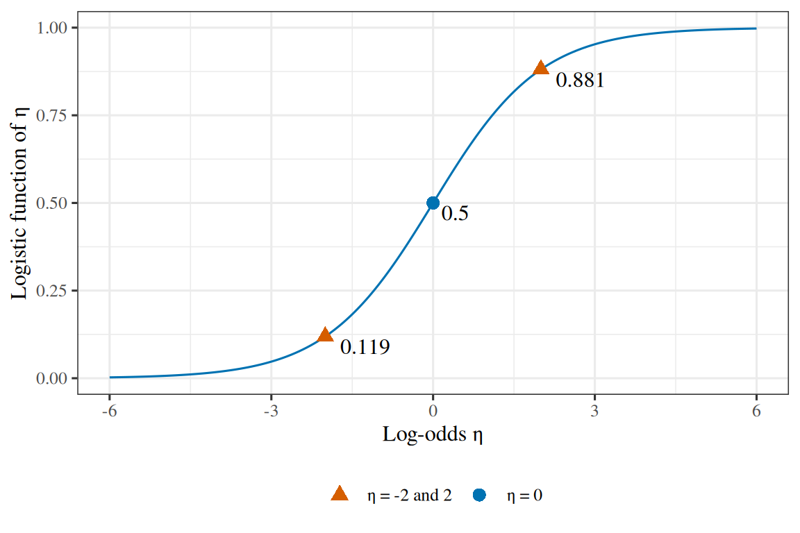
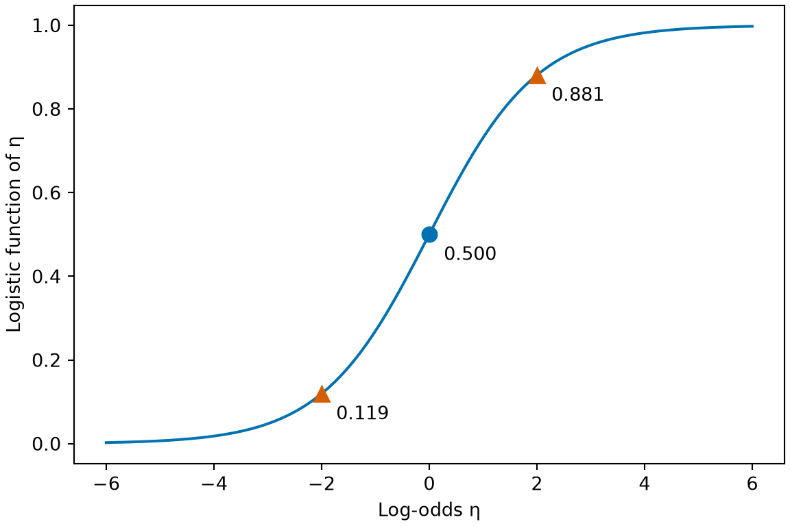
Figure 3: The logistic function turns a score of \(2\) into a high probability, a score of \(-2\) into a low one, and a score of \(0\) into one half (Example 2).

R

(a)

Python

(b)

RemarkRemark 1 (Intercept convention)

Remark 1 (Intercept convention). Logistic regression models the probability of the label as \(\Prf{\Outvar = 1 \mid \vpredvar} = \sigmoidf{\coef{0} + \dprod{\vcoef}{\vpredvar}}\), where \(\coef{0}\) is the intercept and \(\vcoef\) holds the slopes. A formula that shows \(\coef{0}\) separately, as the decision boundary does, uses \(\vcoef\) for the vector of slopes only. The notation choices page explains this convention and how to read a formula that absorbs the intercept into \(\vcoef\).

LemTheorem 1 (Symmetry of the logistic function)

Theorem 1 (Symmetry of the logistic function) For every \(\logodds \in \reals\),

\[ \sigmoidf{-\logodds} = 1 - \sigmoidf{\logodds}. \]

Hence relabelling the classes (\(\outvar \mapsto 1 - \outvar\)) negates every coefficient, including the intercept, and leaves the fitted probabilities unchanged.

ProofProof

Proof. By Solution 8.

ExmExample 3 (Symmetry for a man with a body mass index of 25)

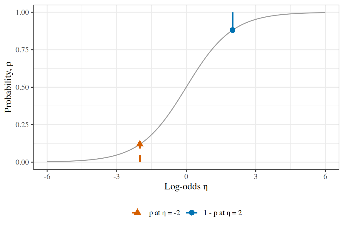
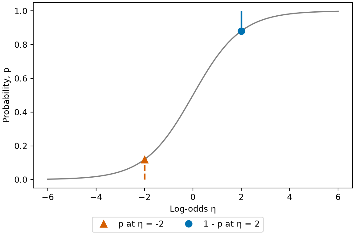
Example 3 (Symmetry for a man with a body mass index of 25) In the model of Example 2, a man with \(\text{bmi} = 25\) has the score \(\logodds = -2.402\). Here \(\sigmoidf{-\logodds} = 0.917\) and \(1 - \sigmoidf{\logodds} = 0.917\) agree. The model gives \(\Prf{\Outvar = 1 \mid \vpredvar} = \sigmoidf{\logodds} = 0.083\) to this man, and therefore \(\Prf{\Outvar = 0 \mid \vpredvar} = \sigmoidf{-\logodds} = 0.917\) to him.

library(ggplot2)
lsy_curve <- data.frame(z = seq(-6, 6, length.out = 241))
lsy_curve$p <- plogis(lsy_curve$z)
lsy_seg <- data.frame(
  z = c(-2, 2),
  from = c(0, plogis(2)),
  to = c(plogis(-2), 1),
  kind = factor(c("p at η = -2", "1 - p at η = 2"), levels = c("p at η = -2", "1 - p at η = 2"))
)
ggplot(lsy_curve, aes(z, p)) +
  geom_line(colour = "grey60") +
  geom_segment(
    data = lsy_seg,
    aes(x = z, xend = z, y = from, yend = to, colour = kind, linetype = kind),
    linewidth = 1
  ) +
  geom_point(
    data = data.frame(z = c(-2, 2), p = plogis(c(-2, 2)), kind = lsy_seg$kind),
    aes(colour = kind, shape = kind), size = 3
  ) +
  scale_colour_manual(values = c("p at η = -2" = "#D55E00", "1 - p at η = 2" = "#0072B2")) +
  scale_linetype_manual(values = c("p at η = -2" = "dashed", "1 - p at η = 2" = "solid")) +
  scale_shape_manual(values = c("p at η = -2" = 17, "1 - p at η = 2" = 16)) +
  labs(x = "Log-odds η", y = "Probability, p", colour = NULL, linetype = NULL, shape = NULL)

import matplotlib.pyplot as plt
import numpy as np
from scipy.special import expit

grid_lsy = np.linspace(-6, 6, 241)
fig, ax = plt.subplots(figsize=(6, 4), layout="constrained")
ax.plot(grid_lsy, expit(grid_lsy), color="grey");
ax.vlines(-2, 0, expit(-2), color="#D55E00", linestyle="--", linewidth=2);
ax.plot(-2, expit(-2), color="#D55E00", marker="^", markersize=8, linestyle="",
        label="p at η = -2");
ax.vlines(2, expit(2), 1, color="#0072B2", linestyle="-", linewidth=2);
ax.plot(2, expit(2), color="#0072B2", marker="o", markersize=8, linestyle="",
        label="1 - p at η = 2");
ax.set_xlabel("Log-odds η");
ax.set_ylabel("Probability, p");
fig.legend(loc="outside lower center", ncol=2);
plt.show()

Figure 4: The logistic function at \(-2\) equals one minus its value at \(2\), so the dashed segment up from \(0\) and the solid segment down from \(1\) have the same length (Example 3).

R

(a)

Python

(b)

LemTheorem 2 (Derivative of the logistic function)

Theorem 2 (Derivative of the logistic function) For every \(\logodds \in \reals\),

\[ \sigmoid'(\logodds) = \sigmoidf{\logodds}\paren{1 - \sigmoidf{\logodds}}. \]

ProofProof

Proof. By Solution 9 and Solution 10.

ExmExample 4 (Slope of the logistic function for a man with a body mass index of 25)

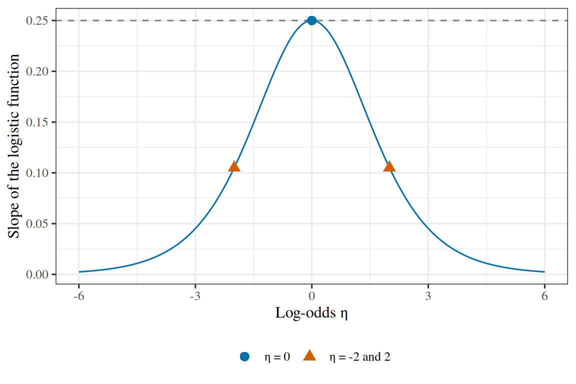
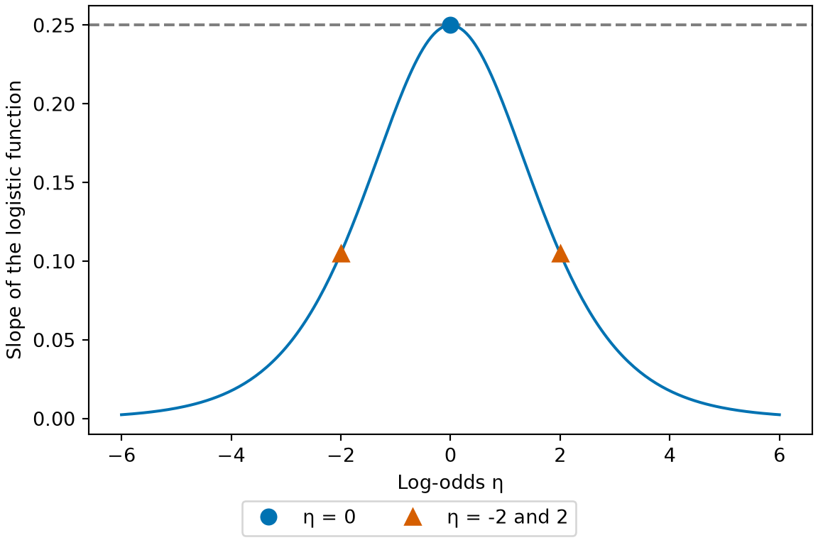
Example 4 (Slope of the logistic function for a man with a body mass index of 25) At the score \(\logodds = -2.402\) of the man with \(\text{bmi} = 25\) in Example 3, the slope of the sigmoid is \(\dexpitf{\logodds} = \sigmoidf{\logodds}\paren{1 - \sigmoidf{\logodds}} = 0.0761\). It is the same at \(-\logodds\), because Theorem 1 swaps the two factors \(\sigmoidf{\logodds}\) and \(1 - \sigmoidf{\logodds}\). At \(\logodds = 0\) the slope is \(\dexpitf{0} = 0.25\), 3.3 times as large.

library(ggplot2)
lde_slope <- function(z) plogis(z) * (1 - plogis(z))
lde_pts <- data.frame(z = c(-2, 0, 2))
lde_pts$slope <- lde_slope(lde_pts$z)
lde_pts$kind <- factor(ifelse(lde_pts$z == 0, "η = 0", "η = -2 and 2"), levels = c("η = 0", "η = -2 and 2"))
ggplot(data.frame(z = c(-6, 6)), aes(z)) +
  geom_hline(yintercept = lde_slope(0), linetype = "dashed", colour = "grey50") +
  geom_function(fun = lde_slope, colour = "#0072B2", n = 241) +
  geom_point(data = lde_pts, aes(y = slope, colour = kind, shape = kind), size = 3) +
  scale_colour_manual(values = c("η = 0" = "#0072B2", "η = -2 and 2" = "#D55E00")) +
  scale_shape_manual(values = c("η = 0" = 16, "η = -2 and 2" = 17)) +
  labs(x = "Log-odds η", y = "Slope of the logistic function", colour = NULL, shape = NULL)

import matplotlib.pyplot as plt
import numpy as np
from scipy.special import expit

def slope_lde(z):
    return expit(z) * (1 - expit(z))

grid_lde = np.linspace(-6, 6, 241)
fig, ax = plt.subplots(figsize=(6, 4), layout="constrained")
ax.axhline(slope_lde(0), color="grey", linestyle="--");
ax.plot(grid_lde, slope_lde(grid_lde), color="#0072B2");
ax.plot(0, slope_lde(0), color="#0072B2", marker="o", markersize=8, linestyle="",
        label="η = 0");
ax.plot([-2, 2], slope_lde(np.array([-2, 2])), color="#D55E00", marker="^", markersize=8,
        linestyle="", label="η = -2 and 2");
ax.set_xlabel("Log-odds η");
ax.set_ylabel("Slope of the logistic function");
fig.legend(loc="outside lower center", ncol=2);
plt.show()

Figure 5: The slope of the logistic function is highest at a score of \(0\), and it is the same at \(-2\) as at \(2\) (Example 4).

R

(a)

Python

(b)

LemTheorem 3 (The logistic function is steepest at zero)

Theorem 3 (The logistic function is steepest at zero) For every \(\logodds \in \reals\), \(\sigmoid'(\logodds) \le 1/4\), with equality if and only if \(\logodds = 0\).

ProofProof

Proof. By Theorem 2, \(\sigmoid'(\logodds) = \sigmoidf{\logodds}\paren{1 - \sigmoidf{\logodds}}\). Completing the square in \(\sigmoidf{\logodds}\) gives

\[ \sigmoidf{\logodds}\paren{1 - \sigmoidf{\logodds}} = \frac{1}{4} - \paren{\sigmoidf{\logodds} - \frac{1}{2}}^2. \]

The square is nonnegative, so \(\sigmoid'(\logodds) \le 1/4\), with equality if and only if \(\sigmoidf{\logodds} = 1/2\). Since the logistic function is strictly increasing with \(\sigmoidf{0} = 1/2\), this happens only at \(\logodds = 0\).

ExmExample 5 (Slope across the body mass indices in the WCGS data)

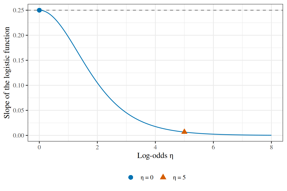
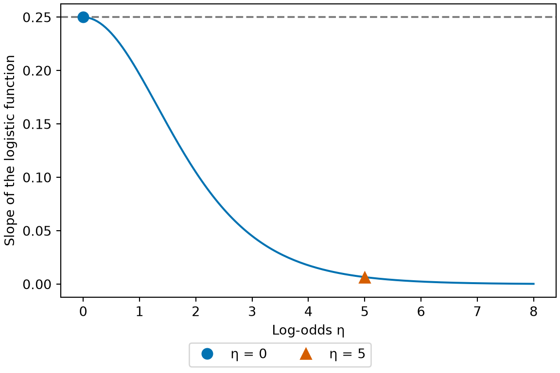
Example 5 (Slope across the body mass indices in the WCGS data) The slope at \(\logodds = 0\) is \(0.25\), the bound of Theorem 3. In the model of Example 2, the body mass indices in the WCGS data run from 11.19 to 38.95, with scores from \(-3.57\) to \(-1.23\). Over these men the slope runs from \(0.0267\) to \(0.1754\), below the bound because no man has a score of \(0\), and smaller the further a score is from \(0\).

library(ggplot2)
ldb_slope <- function(z) plogis(z) * (1 - plogis(z))
ldb_pts <- data.frame(z = c(0, 5))
ldb_pts$slope <- ldb_slope(ldb_pts$z)
ldb_pts$kind <- factor(c("η = 0", "η = 5"), levels = c("η = 0", "η = 5"))
ggplot(data.frame(z = c(0, 8)), aes(z)) +
  geom_hline(yintercept = ldb_slope(0), linetype = "dashed", colour = "grey50") +
  geom_function(fun = ldb_slope, colour = "#0072B2", n = 241) +
  geom_point(data = ldb_pts, aes(y = slope, colour = kind, shape = kind), size = 3) +
  scale_colour_manual(values = c("η = 0" = "#0072B2", "η = 5" = "#D55E00")) +
  scale_shape_manual(values = c("η = 0" = 16, "η = 5" = 17)) +
  labs(x = "Log-odds η", y = "Slope of the logistic function", colour = NULL, shape = NULL)

import matplotlib.pyplot as plt
import numpy as np
from scipy.special import expit

def slope_ldb(z):
    return expit(z) * (1 - expit(z))

grid_ldb = np.linspace(0, 8, 161)
fig, ax = plt.subplots(figsize=(6, 4), layout="constrained")
ax.axhline(slope_ldb(0), color="grey", linestyle="--");
ax.plot(grid_ldb, slope_ldb(grid_ldb), color="#0072B2");
ax.plot(0, slope_ldb(0), color="#0072B2", marker="o", markersize=8, linestyle="", label="η = 0");
ax.plot(5, slope_ldb(5), color="#D55E00", marker="^", markersize=8, linestyle="", label="η = 5");
ax.set_xlabel("Log-odds η");
ax.set_ylabel("Slope of the logistic function");
fig.legend(loc="outside lower center", ncol=2);
plt.show()

Figure 6: The slope of the logistic function falls from its highest value at \(0\) to a value near zero at \(5\), as in Example 5.

R

(a)

Python

(b)

VideosWatch

• Hastie and Tibshirani introduce logistic regression [4], video 4.2.
• Hutchinson teaches logistic regression (17 min) [1].
• Starmer introduces logistic regression [5].

ReadingRead

GeeksforGeeks explains:

• logistic regression [6]
• the sigmoid function [7]

ReadingRead

The University of Washington’s CSE 446 slides cover classification and logistic regression [8], Lecture 13.

ExrExercise 12 (What the coefficients do to the surface)

Exercise 12 (What the coefficients do to the surface) Set \(\coef{0} = 0\), so the surface \(p(\vx) = \sigmoid(\dprod{\vcoef}{\vx})\) passes through \(1/2\) at the origin, and let \(\vcoef \neq \vzero\).

Compare the surfaces for \(\vcoef\) and \(10\vcoef\). What is the same about them?

SolutionSolution 12

Solution 12. Same shape, steeper. Both surfaces rise from \(0\) to \(1\) along the same direction \(\vcoef\) and are constant on the same family of parallel hyperplanes \(\dprod{\vcoef}{\vx} = c\), because \(10\dprod{\vcoef}{\vx} = 10c\) is constant exactly when \(\dprod{\vcoef}{\vx}\) is.

ExrExercise 13 (What the coefficients do to the surface (part 2))

Exercise 13 (What the coefficients do to the surface (part 2)) Use the setup of Exercise 12.

What is different about them?

SolutionSolution 13

Solution 13. The surfaces differ in how fast they rise. Going from \(p = 0.02\) to \(p = 0.98\) corresponds to going from \(\logodds = \log(0.02/0.98)\) to \(\logodds = \log(0.98/0.02)\), an interval of length \(2\log 49 \approx 7.78\) in \(\logodds\). Since \(\logodds = \dprod{\vcoef}{\vx}\), that range is covered by a distance \(7.78/\norm{\vcoef}\) along \(\vcoef\) — so \(10\vcoef\) covers it in one-tenth the distance required by \(\vcoef\).

ExrExercise 14 (What the coefficients do to the surface (part 3))

Exercise 14 (What the coefficients do to the surface (part 3)) Use the setup of Exercise 12.

Give the set of points where the two agree.

SolutionSolution 14

Solution 14. They agree exactly on the hyperplane \(\dprod{\vcoef}{\vx} = 0\), where both read \(1/2\), and nowhere else: for \(\logodds \neq 0\), \(\sigmoid(10\logodds) \neq \sigmoid(\logodds)\) since \(\sigmoid\) is injective.

ExrExercise 15 (What the coefficients do to the surface (part 4))

Exercise 15 (What the coefficients do to the surface (part 4)) Use the setup of Exercise 12.

Compare the surfaces for \(\vcoef\) and \(\vcoef/10\).

SolutionSolution 15

Solution 15. Same shape, flatter, by the same argument with the factor inverted. As the scale falls toward zero the surface flattens toward the constant \(1/2\), which is the model that ignores \(\vx\) altogether and predicts the class prevalence.

ExrExercise 16 (What the coefficients do to the surface (part 5))

Exercise 16 (What the coefficients do to the surface (part 5)) Use the setup of Exercise 12.

Compare the surfaces for \(\vcoef\) and \(-\vcoef\).

SolutionSolution 16

Solution 16. The surface is reflected. \(\sigmoid(-\logodds) = 1 - \sigmoid(\logodds)\) from Exercise 7, so the surface for \(-\vcoef\) is \(1\) minus the surface for \(\vcoef\): it falls where the other rises, at the same rate, about the same hyperplane.

This is the class relabelling of Exercise 8 seen geometrically.

ExrExercise 17 (What the coefficients do to the surface (part 6))

Exercise 17 (What the coefficients do to the surface (part 6)) Use the setup of Exercise 12.

From Exercise 12 to Exercise 16, separate what \(\vcoef\) encodes into a direction and a magnitude, and say in one sentence what each controls.

SolutionSolution 17

Solution 17. Direction. \(\vcoef/\norm{\vcoef}\) fixes which way the probability increases, and so fixes the orientation of the decision boundary — the boundary is perpendicular to it (Exercise 24).

Magnitude. \(\norm{\vcoef}\) fixes how sharply the probability turns over as \(\vx\) crosses that boundary, and so fixes the model’s confidence: large \(\norm{\vcoef}\) is a model that commits to \(0\) or \(1\) just outside the boundary, small \(\norm{\vcoef}\) a model that gives intermediate probabilities.

Because the magnitude is a separate quantity from the direction, Exercise 92 is possible, where the direction is determined and the magnitude grows without bound, and \(\lpnorm{2}\) regularization restricts it, as Solution 96 of that exercise works out.

ExrExercise 18 (What the coefficients do to the surface (part 7))

Exercise 18 (What the coefficients do to the surface (part 7)) Use the setup of Exercise 12.

Now allow a nonzero intercept \(\coef{0}\). State how the surface changes, and give the point along the direction \(\vcoef\) at which the surface equals \(1/2\).

SolutionSolution 18

Solution 18. Nothing about direction or steepness changes. \(\coef{0}\) shifts the surface along \(\vcoef\) without rotating or scaling it, so the family of parallel hyperplanes is unchanged and only the hyperplane on which the probability equals \(1/2\) moves.

That hyperplane is \(\coef{0} + \dprod{\vcoef}{\vx} = 0\). Along the direction \(\vcoef\), setting \(\vx = t\,\vcoef/\norm{\vcoef}\), the surface equals \(1/2\) at \(t = -\coef{0}/\norm{\vcoef}\).

So \(\coef{0}\) is a signed distance in units of \(1/\norm{\vcoef}\), which is why it is reported alongside the other coefficients but interpreted differently: it is the log odds at \(\vx = \vzero\), which is a meaningful quantity only if \(\vx = \vzero\) is a case that could occur. Centring the features makes it one.

VideosWatch

• Andrew Ng derives logistic regression, from 46:18 [9], Lecture 3.
• Weinberger introduces logistic regression, from 26:12 [10], Lecture 11.

3 What the coefficients mean

A coefficient in a linear regression is a change in the response per unit change in a predictor. Here the response is a probability, and \(\sigmoid\) is not linear, so a unit change in a predictor does not change the probability by a fixed amount.

The log odds are the quantity the model makes linear. Deriving which transformation of a probability a linear model can act on yields the sigmoid rather than assuming it.

ExrExercise 19 (Deriving the sigmoid instead of choosing it)

Exercise 19 (Deriving the sigmoid instead of choosing it) Exercise 4 requires a function that maps \(\dprod{\vcoef}{\vx}\) into \((0,1)\). Many functions map \(\reals\) into \((0,1)\), so choosing one requires a modelling criterion. Rather than choosing a function that maps into \((0,1)\) and then asking how to interpret the parameters, we specify what the linear score \(\dprod{\vcoef}{\vx}\) represents and solve for the function.

Let \(p(\vx) = \Pr[Y = 1 \mid \vx]\).

The odds of an event of probability \(p\) are \(p/(1-p)\). State the range of the odds as \(p\) varies over \((0,1)\), and the range of the log-odds \(\log\frac{p}{1-p}\).

SolutionSolution 19

Solution 19. As \(p\) varies over \((0,1)\), the odds \(p/(1-p)\) range over \((0, \infty)\): the numerator approaches \(0\) as \(p \to 0\), and the denominator approaches \(0\) as \(p \to 1\). The logarithm maps \((0,\infty)\) bijectively onto \((-\infty, \infty)\).

So the log-odds transform maps a probability in \((0, 1)\) onto the entire real line \((-\infty, \infty)\).

ExrExercise 20 (Deriving the sigmoid instead of choosing it (part 2))

Exercise 20 (Deriving the sigmoid instead of choosing it (part 2)) Use the setup of Exercise 19.

A linear score \(\dprod{\vcoef}{\vx}\) ranges over \((-\infty, \infty)\). Given Exercise 19, state the modelling assumption that equates the linear score to a function of \(p\) with the same range \((-\infty, \infty)\), without truncation or clipping.

SolutionSolution 20

Solution 20. The assumption is that the log odds are linear in the features:

\[\log \frac{p(\vx)}{1 - p(\vx)} = \dprod{\vcoef}{\vx}\]

Both sides have range \((-\infty, \infty)\), so the equation can hold for every \(\vx \in \reals^{\ninputvars}\) without clipping or restricting \(\vcoef\). This linearity of the log odds is the defining modeling assumption of logistic regression; the sigmoid formula for \(p(\vx)\) follows by algebra.

ExrExercise 21 (Deriving the sigmoid instead of choosing it (part 3))

Exercise 21 (Deriving the sigmoid instead of choosing it (part 3)) Use the setup of Exercise 19.

Solve \(\log\dfrac{p}{1-p} = \logodds\) for \(p\). Show every step.

SolutionSolution 21

Solution 21. Exponentiate, then clear the denominator:

\[\frac{p}{1-p} = e^{\logodds}\] \[p = (1-p)\,e^{\logodds}\] \[p = e^{\logodds} - p\,e^{\logodds}\] \[p + p\,e^{\logodds} = e^{\logodds}\] \[p\,(1 + e^{\logodds}) = e^{\logodds}\] \[p = \frac{e^{\logodds}}{1 + e^{\logodds}}\]

Divide numerator and denominator by \(e^{\logodds}\):

\[ \begin{aligned} p &= \frac{1}{1 + e^{-\logodds}} \\ &= \sigmoid(\logodds) \end{aligned} \]

Both expressions for \(\sigmoid(\logodds)\) appear in the literature; the second form \(1/(1 + e^{-\logodds})\) avoids floating-point overflow for large positive \(\logodds\), where \(e^{\logodds}\) overflows.

ExrExercise 22 (Deriving the sigmoid instead of choosing it (part 4))

Exercise 22 (Deriving the sigmoid instead of choosing it (part 4)) Use the setup of Exercise 19.

The function you obtained is the logistic function, \(\sigmoid\). State in one sentence what the coefficient \(\coef{j}\) therefore represents.

SolutionSolution 22

Solution 22. \(\coef{j}\) is the change in the log odds of \(\Outvar = 1\) per one-unit increase in \(\predvar_j\), holding the other features fixed. Equivalently, on the odds scale, increasing \(\predvar_j\) by one unit multiplies the odds by \(\e{\coef{j}}\) (Theorem 5).

A coefficient of \(0.693 \approx \log 2\) multiplies the odds by \(2\); a coefficient of \(0\) leaves them unchanged; a negative coefficient multiplies them by a factor in \((0, 1)\).

ExrExercise 23 (Deriving the sigmoid instead of choosing it (part 5))

Exercise 23 (Deriving the sigmoid instead of choosing it (part 5)) Use the setup of Exercise 19.

The earlier parts, Exercise 19 to Exercise 22, do not show that the assumption in Exercise 20 holds for any given dataset. Describe how to check this assumption empirically on a dataset, and give one example in which you would expect it to fail.

SolutionSolution 23

Solution 23. It is a modelling assumption that can be checked against data. The assumption states that the log odds are linear in each feature, so plotting the empirical log odds against \(\predvar_j\) — binning \(\predvar_j\), computing the proportion \(\hat p\) of observations with \(\outvar = 1\) in each bin, and plotting \(\log\frac{\hat p}{1 - \hat p}\) against the bin midpoint — should yield points scattered around a straight line. Systematic curvature indicates that the log odds are not linear in \(x_j\).

This assumption fails whenever a feature has an interior optimum. For blood pressure and mortality risk, both very low and very high blood pressure are associated with elevated risk, so the empirical log odds are U-shaped and no linear function of blood pressure alone fits. Adding a quadratic feature \(\predvar_j^2\) restores linearity in the parameters, because the model assumes linearity in the features rather than in the raw measurements.

The odds of an event are defined in the probability prerequisites.

ExmExample 6 (Odds of coronary heart disease in the WCGS data)

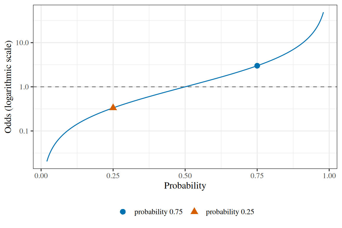
Example 6 (Odds of coronary heart disease in the WCGS data) In the WCGS data of Exercise 1, the proportion of men with an incident case of coronary heart disease is \(\prob = 0.081\). The odds are \(\odds = \prob / (1 - \prob) = 0.089\), about \(1\) to \(11.3\).

library(ggplot2)
od_curve <- data.frame(prob = seq(0.02, 0.98, length.out = 241))
od_curve$odds <- od_curve$prob / (1 - od_curve$prob)
od_pts <- data.frame(prob = c(0.25, 0.75))
od_pts$odds <- od_pts$prob / (1 - od_pts$prob)
od_pts$kind <- factor(c("probability 0.25", "probability 0.75"),
                      levels = c("probability 0.75", "probability 0.25"))
ggplot(od_curve, aes(prob, odds)) +
  geom_hline(yintercept = 1, linetype = "dashed", colour = "grey50") +
  geom_line(colour = "#0072B2") +
  geom_point(data = od_pts, aes(colour = kind, shape = kind), size = 3) +
  scale_y_log10() +
  scale_colour_manual(values = c("probability 0.75" = "#0072B2", "probability 0.25" = "#D55E00")) +
  scale_shape_manual(values = c("probability 0.75" = 16, "probability 0.25" = 17)) +
  labs(x = "Probability", y = "Odds (logarithmic scale)", colour = NULL, shape = NULL)

import matplotlib.pyplot as plt
import numpy as np

prob_od = np.linspace(0.02, 0.98, 241)
fig, ax = plt.subplots(figsize=(6, 4), layout="constrained")
ax.axhline(1, color="grey", linestyle="--");
ax.plot(prob_od, prob_od / (1 - prob_od), color="#0072B2");
ax.plot(0.75, 0.75 / 0.25, color="#0072B2", marker="o", markersize=8, linestyle="",
        label="probability 0.75");
ax.plot(0.25, 0.25 / 0.75, color="#D55E00", marker="^", markersize=8, linestyle="",
        label="probability 0.25");
ax.set_yscale("log");
ax.set_xlabel("Probability");
ax.set_ylabel("Odds (logarithmic scale)");
fig.legend(loc="outside lower center", ncol=2);
plt.show()

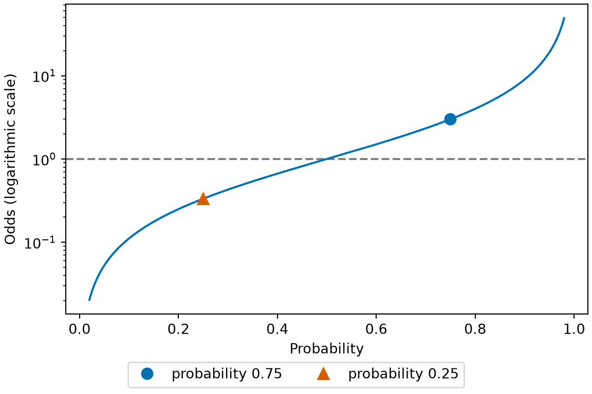
Figure 7: The odds of Example 6 against the probability, on a logarithmic scale. A probability and its complement have odds that are reciprocals, so they lie at equal distances on either side of the odds of \(1\).

R

(a)

Python

(b)

The log-odds, also called the logit, are defined there too.

ExmExample 7 (Log-odds of coronary heart disease in the WCGS data)

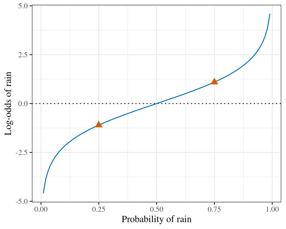
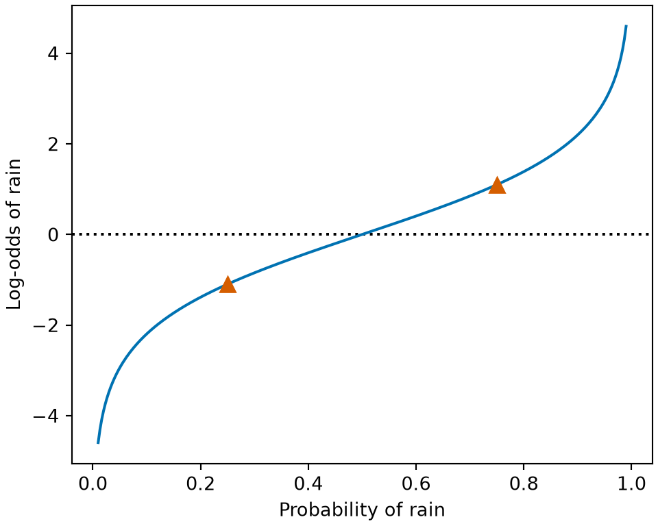
Example 7 (Log-odds of coronary heart disease in the WCGS data) In the WCGS data of Exercise 1, the proportion with coronary heart disease is \(\prob = 0.081\) and the odds are \(0.089\) (Example 6). The log-odds are \(\logodds = -2.422\). The log-odds are negative because the probability is below \(1/2\).

library(ggplot2)
lo_marks <- data.frame(prob = c(0.25, 0.75))
lo_marks$logodds <- log(lo_marks$prob / (1 - lo_marks$prob))
ggplot(data.frame(prob = c(0.01, 0.99)), aes(prob)) +
  geom_hline(yintercept = 0, linetype = "dotted") +
  geom_function(fun = function(p) log(p / (1 - p)), colour = "#0072B2") +
  geom_point(data = lo_marks, aes(prob, logodds), colour = "#D55E00", shape = 17, size = 3) +
  labs(x = "Probability of rain", y = "Log-odds of rain")

import matplotlib.pyplot as plt
import numpy as np

def log_odds_lo(prob):
    return np.log(prob / (1 - prob))

grid_lo = np.linspace(0.01, 0.99, 300)
marks_lo = np.array([0.25, 0.75])
fig, ax = plt.subplots(figsize=(5, 4), layout="constrained")
ax.axhline(0, color="black", linestyle=":");
ax.plot(grid_lo, log_odds_lo(grid_lo), color="#0072B2");
ax.plot(marks_lo, log_odds_lo(marks_lo), color="#D55E00", marker="^", markersize=8, linestyle="");
ax.set_xlabel("Probability of rain");
ax.set_ylabel("Log-odds of rain");
plt.show()

Figure 8: The log-odds of rain from Example 7 against its probability, with the example’s two probabilities marked. The log-odds are \(0\) at probability one half and change sign on either side of it.

R

(a)

Python

(b)

LemTheorem 4 (Probability from the log-odds)

Theorem 4 (Probability from the log-odds) If the log-odds of an event are \(\logodds\), its probability is

\[ \prob = \sigmoidf{\logodds} = \frac{1}{1 + \e{-\logodds}}. \]

Hence the logistic regression model \(\log \dfrac{\prob(\vpredvar)}{1 - \prob(\vpredvar)} = \dprod{\vcoef}{\vpredvar}\) is the same as \(\prob(\vpredvar) = \sigmoidf{\dprod{\vcoef}{\vpredvar}}\).

ProofProof

Proof. By Solution 21 and Solution 22.

ExmExample 8 (From log-odds to probability in the WCGS data)

Example 8 (From log-odds to probability in the WCGS data) The log-odds of coronary heart disease in the WCGS data are \(\logodds = -2.422\) (Example 7). These log-odds give \(\prob = \sigmoidf{\logodds} = 0.081\), the proportion of Example 6, as they must.

LemTheorem 5 (The odds multiplier of a coefficient)

Theorem 5 (The odds multiplier of a coefficient) In the logistic regression model \(\prob(\vpredvar) = \sigmoidf{\dprod{\vcoef}{\vpredvar}}\), increasing \(\predvar_j\) by one unit, holding the other predictors fixed, multiplies the odds by \(\e{\coef{j}}\).

ProofProof

Proof. By Theorem 4 the log-odds are \(\logodds = \dprod{\vcoef}{\vpredvar}\), so the odds are \(\e{\logodds}\). Increasing \(\predvar_j\) by one unit, with the other predictors fixed, changes the score from \(\logodds\) to \(\logodds + \coef{j}\). The odds therefore change from \(\e{\logodds}\) to \(\e{\logodds + \coef{j}} = \e{\logodds} \e{\coef{j}}\), a factor of \(\e{\coef{j}}\).

ExmExample 9 (The odds multiplier of body mass index)

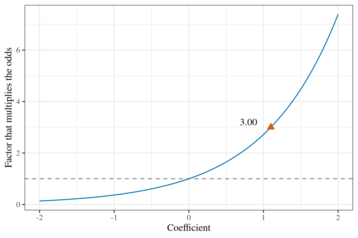
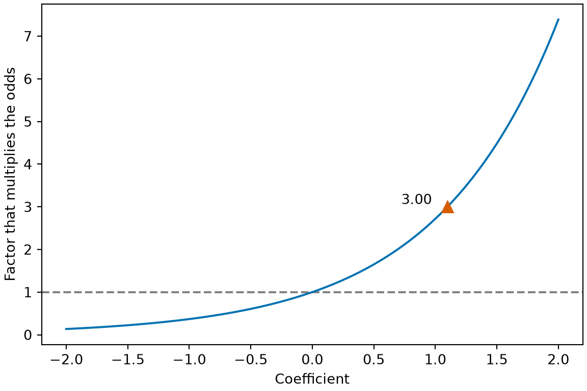
Example 9 (The odds multiplier of body mass index) In the model of Example 2, the coefficient of bmi is \(\coef{1} = 0.084\). One more unit of body mass index multiplies the odds of coronary heart disease by \(\e{\coef{1}} = 1.088\), an increase of about 8.8%.

library(ggplot2)
om_curve <- data.frame(coef = seq(-2, 2, length.out = 241))
om_curve$factor <- exp(om_curve$coef)
om_pt <- data.frame(coef = 1.099, factor = exp(1.099))
ggplot(om_curve, aes(coef, factor)) +
  geom_hline(yintercept = 1, linetype = "dashed", colour = "grey50") +
  geom_line(colour = "#0072B2") +
  geom_point(data = om_pt, colour = "#D55E00", shape = 17, size = 3) +
  geom_text(data = om_pt, aes(label = sprintf("%.2f", factor)), nudge_x = -0.3, nudge_y = 0.2) +
  labs(x = "Coefficient", y = "Factor that multiplies the odds")

import matplotlib.pyplot as plt
import numpy as np

coef_om = np.linspace(-2, 2, 241)
fig, ax = plt.subplots(figsize=(6, 4), layout="constrained")
ax.axhline(1, color="grey", linestyle="--");
ax.plot(coef_om, np.exp(coef_om), color="#0072B2");
ax.plot(1.099, np.exp(1.099), color="#D55E00", marker="^", markersize=8, linestyle="");
ax.annotate(f"{np.exp(1.099):.2f}", (1.099, np.exp(1.099)), xytext=(-34, 2),
            textcoords="offset points");
ax.set_xlabel("Coefficient");
ax.set_ylabel("Factor that multiplies the odds");
plt.show()

Figure 9: The factor by which a coefficient multiplies the odds, as in Example 9. A coefficient of \(0\) leaves the odds unchanged, and a coefficient of \(1.099\) triples them.

R

(a)

Python

(b)

CorCorollary 1 (The odds ratio of a coefficient)

Corollary 1 (The odds ratio of a coefficient) Let:

• \(\vpredvar\) be a vector of predictors in the logistic model \(\prob(\vpredvar) = \sigmoidf{\dprod{\vcoef}{\vpredvar}}\).
• \(\vpredvar'\) be the same vector with \(\predvar_j\) increased by one unit.

Then the odds ratio of \(\vpredvar'\) compared with \(\vpredvar\) is

\[ \ror = \e{\coef{j}}. \]

ProofProof

Proof. By Theorem 5 the odds at \(\vpredvar'\) are \(\e{\coef{j}}\) times the odds at \(\vpredvar\). The odds ratio is the odds at \(\vpredvar'\) divided by the odds at \(\vpredvar\). That quotient is \(\e{\coef{j}}\).

ExmExample 10 (The odds ratio for body mass index)

Example 10 (The odds ratio for body mass index) In the model of Example 2, take \(\vpredvar\) to be a man with \(\text{bmi} = 25\) and \(\vpredvar'\) a man with \(\text{bmi} = 26\).

wcgs_odds <- function(bmi) {
  p <- unname(predict(wcgs_logit, data.frame(bmi = bmi), type = "response"))
  p / (1 - p)
}
c(odds_25 = wcgs_odds(25), odds_26 = wcgs_odds(26), ratio = wcgs_odds(26) / wcgs_odds(25))

   odds_25    odds_26      ratio 
0.09055613 0.09851816 1.08792371 

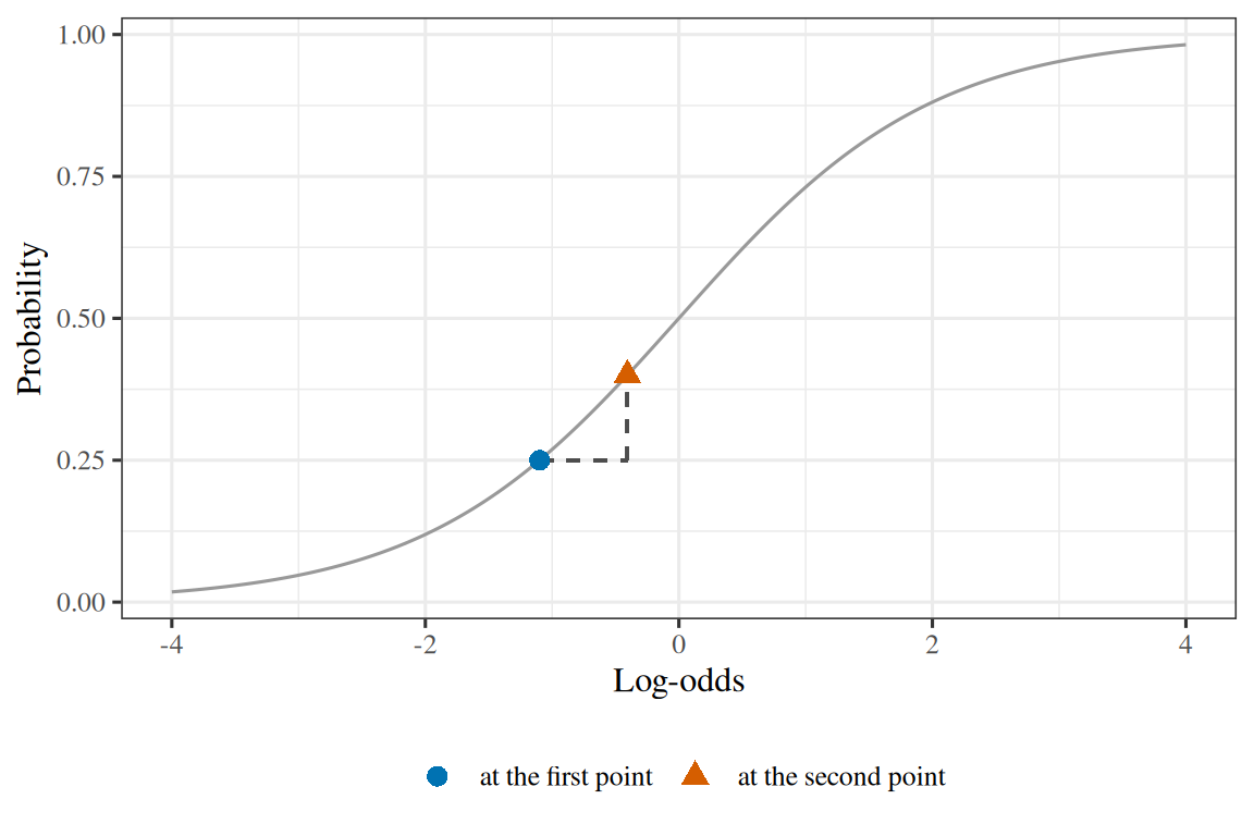
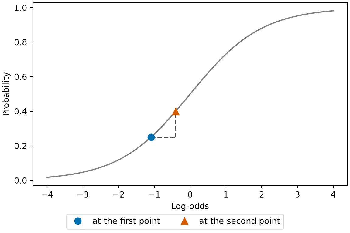
Their odds are \(0.0906\) and \(0.0985\), so the odds ratio is \(\ror = 1.088\). This equals \(\e{\coef{1}} = 1.088\), as Corollary 1 states.

library(ggplot2)
orc_curve <- data.frame(logodds = seq(-4, 4, length.out = 241))
orc_curve$prob <- plogis(orc_curve$logodds)
orc_pts <- data.frame(logodds = c(log(1 / 3), log(1 / 3) + 0.693))
orc_pts$prob <- plogis(orc_pts$logodds)
orc_pts$kind <- factor(c("at the first point", "at the second point"),
                       levels = c("at the first point", "at the second point"))
ggplot(orc_curve, aes(logodds, prob)) +
  geom_line(colour = "grey60") +
  geom_segment(
    x = orc_pts$logodds[1], xend = orc_pts$logodds[2], y = orc_pts$prob[1], yend = orc_pts$prob[1],
    linetype = "dashed", colour = "grey30"
  ) +
  geom_segment(
    x = orc_pts$logodds[2], xend = orc_pts$logodds[2], y = orc_pts$prob[1], yend = orc_pts$prob[2],
    linetype = "dashed", colour = "grey30"
  ) +
  geom_point(data = orc_pts, aes(colour = kind, shape = kind), size = 3) +
  scale_colour_manual(values = c("at the first point" = "#0072B2", "at the second point" = "#D55E00")) +
  scale_shape_manual(values = c("at the first point" = 16, "at the second point" = 17)) +
  labs(x = "Log-odds", y = "Probability", colour = NULL, shape = NULL)

import matplotlib.pyplot as plt
import numpy as np
from scipy.special import expit

logodds_orc = np.linspace(-4, 4, 241)
first_orc = np.log(1 / 3)
second_orc = first_orc + 0.693
fig, ax = plt.subplots(figsize=(6, 4), layout="constrained")
ax.plot(logodds_orc, expit(logodds_orc), color="grey");
ax.hlines(expit(first_orc), first_orc, second_orc, color="#4d4d4d", linestyle="--");
ax.vlines(second_orc, expit(first_orc), expit(second_orc), color="#4d4d4d", linestyle="--");
ax.plot(first_orc, expit(first_orc), color="#0072B2", marker="o", markersize=8, linestyle="",
        label="at the first point");
ax.plot(second_orc, expit(second_orc), color="#D55E00", marker="^", markersize=8, linestyle="",
        label="at the second point");
ax.set_xlabel("Log-odds");
ax.set_ylabel("Probability");
fig.legend(loc="outside lower center", ncol=2);
plt.show()

Figure 10: The two points of Example 10 on the logistic function. A coefficient of \(0.693\) moves the log-odds to the right by \(0.693\), which doubles the odds.

R

(a)

Python

(b)

LemTheorem 6 (Linear log odds give the sigmoid)

Theorem 6 (Linear log odds give the sigmoid) If the log odds of \(Y = 1\) are \(\logodds\), that is, \(\log\frac{p}{1-p} = \logodds\) for a probability \(p \in (0, 1)\), then

\[ p = \frac{\e{\logodds}}{1 + \e{\logodds}} = \frac{1}{1 + \e{-\logodds}} = \sigmoid(\logodds). \]

In particular, if the log odds are linear in the features, \(\logodds = \dprod{\vcoef}{\vx}\), then \(\Pr[Y = 1 \mid \vx] = \sigmoidf{\dprod{\vcoef}{\vx}}\).

ProofProof

Proof. This is the solution to Exercise 21: see Solution 21.

ExmExample 11 (From log-odds back to a probability)

Example 11 (From log-odds back to a probability) For the man with \(\text{bmi} = 25\) of Example 2, the odds of coronary heart disease are \(\odds = 0.0906\) (Example 10), so the log-odds are \(\logodds = \log \odds = -2.402\).

sg_z <- log(wcgs_odds(25))
c(log_odds = sg_z, sigmoid = plogis(sg_z), direct = wcgs_odds(25) / (1 + wcgs_odds(25)))

   log_odds     sigmoid      direct 
-2.40178544  0.08303665  0.08303665 

By Theorem 6, \(\prob = \sigmoidf{\logodds} = 1 / (1 + \e{-\logodds}) = 0.083\), which equals the probability \(\odds / (1 + \odds)\) that those odds always give.

library(ggplot2)
sgf_curve <- data.frame(z = seq(-4, 4, length.out = 241))
sgf_curve$p <- plogis(sgf_curve$z)
sgf_pt <- data.frame(z = sg_z, p = plogis(sg_z))
ggplot(sgf_curve, aes(z, p)) +
  geom_line(colour = "grey60") +
  geom_segment(
    data = sgf_pt, aes(x = z, xend = z, y = 0, yend = p),
    colour = "#D55E00", linetype = "dashed"
  ) +
  geom_segment(
    data = sgf_pt, aes(x = -4, xend = z, y = p, yend = p),
    colour = "#D55E00", linetype = "dashed"
  ) +
  geom_point(data = sgf_pt, colour = "#D55E00", shape = 17, size = 3) +
  labs(x = "Log odds", y = "Probability")

import matplotlib.pyplot as plt
import numpy as np
from scipy.special import expit

z_sgf = float(r.sg_z)
grid_sgf = np.linspace(-4, 4, 241)
fig, ax = plt.subplots(figsize=(6, 4), layout="constrained")
ax.plot(grid_sgf, expit(grid_sgf), color="grey");
ax.vlines(z_sgf, 0, expit(z_sgf), color="#D55E00", linestyle="--");
ax.hlines(expit(z_sgf), -4, z_sgf, color="#D55E00", linestyle="--");
ax.plot(z_sgf, expit(z_sgf), color="#D55E00", marker="^", markersize=8, linestyle="");
ax.set_xlabel("Log odds");
ax.set_ylabel("Probability");
plt.show()

Figure 11: The logistic function takes the log odds \(\log 3\) of Example 11 back to the probability \(3/4\).

R

(a)

Python

(b)

VideosWatch

• Hastie and Tibshirani fit logistic regression with several predictors [4], video 4.3.
• Starmer explains odds and log odds [11], odds ratios [12], and what the coefficients mean [13].

ReadingRead

GeeksforGeeks explains log odds [14].

4 Where the boundary is

Turning a probability into a decision means choosing a threshold. The set of points where the model is exactly at the threshold is its decision boundary (Definition 2), and for logistic regression it is a hyperplane.

DefDefinition 2 (Decision boundary)

Definition 2 (Decision boundary) The decision boundary of a classifier is the set of feature vectors where it is exactly undecided between two predictions. For a probabilistic classifier with threshold \(\thresh\), it is the set where the predicted probability equals \(\thresh\); for logistic regression at \(\thresh = 1/2\), it is \(\set{\vpredvar : \coef{0} + \dprod{\vcoef}{\vpredvar} = 0}\).

ExmExample 12 (A boundary in two features)

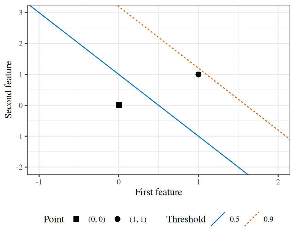
Example 12 (A boundary in two features) Let \(\coef{0} = -1\), \(\coef{1} = 2\), and \(\coef{2} = 1\). The boundary \(-1 + 2 \predvar_1 + \predvar_2 = 0\) is the line \(\predvar_2 = 1 - 2 \predvar_1\). The point \((1, 1)\) has score \(2\) and is on the side predicted \(1\), while \((0, 0)\) has score \(-1\) and is on the other side.

library(ggplot2)

xor_df <- expand.grid(x1 = c(-1, 1), x2 = c(-1, 1))
xor_df$class <- ifelse(xor_df$x1 * xor_df$x2 > 0, "Cross", "Circle")

ggplot(xor_df) +
  aes(x1, x2, shape = class, colour = class) +
  geom_hline(yintercept = 0, colour = "grey70") +
  geom_vline(xintercept = 0, colour = "grey70") +
  geom_point(size = 4, stroke = 1.2) +
  scale_shape_manual(values = c(Circle = 1, Cross = 4)) +
  scale_colour_manual(values = c(Circle = "#0072B2", Cross = "#D55E00")) +
  coord_fixed(xlim = c(-2, 2), ylim = c(-2, 2)) +
  labs(x = "Feature 1, x1", y = "Feature 2, x2", shape = NULL, colour = NULL)

import itertools

import matplotlib.pyplot as plt
import numpy as np

corners = np.array(list(itertools.product([-1, 1], repeat=2)))
is_cross = corners[:, 0] * corners[:, 1] > 0

fig, ax = plt.subplots(figsize=(3.8, 3.2), layout="constrained")
ax.axhline(0, color="lightgrey");
ax.axvline(0, color="lightgrey");
ax.scatter(*corners[~is_cross].T, marker="o", facecolors="none", s=70,
           edgecolors="#0072B2", linewidths=1.5, label="Circle");
ax.scatter(*corners[is_cross].T, marker="x", s=70, color="#D55E00",
           linewidths=1.5, label="Cross");
ax.set_xlim(-2, 2);
ax.set_ylim(-2, 2);
ax.set_aspect("equal");
ax.set_xlabel("Feature 1, x1");
ax.set_ylabel("Feature 2, x2");
fig.legend(loc="outside lower center", ncol=2, frameon=False);
plt.show()

Figure 12: Four points arranged so that the class is the sign of \(x_1 x_2\). No straight line in the plane separates the circles from the crosses.

R

(a)

Python

(b)

ExrExercise 24 (The boundary is a hyperplane)

Exercise 24 (The boundary is a hyperplane) A classifier must return a class label rather than a probability, so we apply a threshold to the predicted probability. Using the threshold \(1/2\), predict \(\hy = 1\) when \(p(\vx) = \sigmoid(\coef{0} + \dprod{\vcoef}{\vx}) > 1/2\).

Show that this rule is equivalent to a condition that is linear in \(\vx\), and state that condition.

SolutionSolution 24

Solution 24. \(\sigmoid\) is strictly increasing and \(\sigmoid(0) = 1/2\), so \(\sigmoid(\logodds) > 1/2 \iff \logodds > 0\). Hence

\[\hy = 1 \iff \coef{0} + \dprod{\vcoef}{\vx} > 0\]

which is linear in \(\vx\). The sigmoid has vanished entirely: it decides how confident the model is, and contributes nothing to which class is predicted.

ExrExercise 25 (The boundary is a hyperplane (part 2))

Exercise 25 (The boundary is a hyperplane (part 2)) Use the setup of Exercise 24.

The set of \(\vx\) where the predicted probability equals the threshold is the decision boundary. Identify this geometric set, and give its normal vector.

SolutionSolution 25

Solution 25. A hyperplane: the set \(\{\vx : \coef{0} + \dprod{\vcoef}{\vx} = 0\}\). In two dimensions it is a line, in three a plane, in \(\ninputvars\) dimensions a flat \((\ninputvars-1)\)-dimensional sheet.

Its normal vector is \(\vcoef\). That is the geometric content of Exercise 17: the direction of \(\vcoef\) is the direction perpendicular to the boundary, which is why rescaling \(\vcoef\) leaves the boundary alone.

ExrExercise 26 (The boundary is a hyperplane (part 3))

Exercise 26 (The boundary is a hyperplane (part 3)) Use the setup of Exercise 24.

Suppose instead the cost of a false negative is nine times the cost of a false positive, so you threshold at \(p > 0.1\) rather than \(p > 0.5\). Give the new boundary, and say precisely how it differs from the old one.

SolutionSolution 26

Solution 26. Threshold at \(p > t\) rather than \(p > 1/2\):

\[\sigmoid(\logodds) > t \iff \logodds > \sigmoid^{-1}(t) = \log\frac{t}{1-t}\]

so the boundary is \(\coef{0} + \dprod{\vcoef}{\vx} = \log\frac{t}{1-t}\).

At \(t = 0.1\) that is \(\log(1/9) = -2.197\). The boundary is the same hyperplane translated: same normal vector, same orientation, shifted along \(\vcoef\) by \(2.197/\norm{\vcoef}\) in the direction that enlarges the region predicted \(1\).

Two consequences follow. First, changing the threshold does not require refitting the model: one set of fitted probabilities supports every threshold, so two users with different misclassification costs can apply different thresholds to the same fitted model. Second, the cost ratio enters the boundary equation only through the constant term \(\log\frac{t}{1-t}\), so changing the threshold shifts the intercept of the boundary without changing \(\vcoef\).

ExrExercise 27 (The boundary is a hyperplane (part 4))

Exercise 27 (The boundary is a hyperplane (part 4)) Use the setup of Exercise 24.

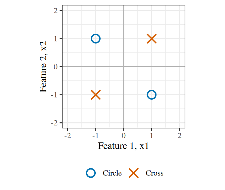
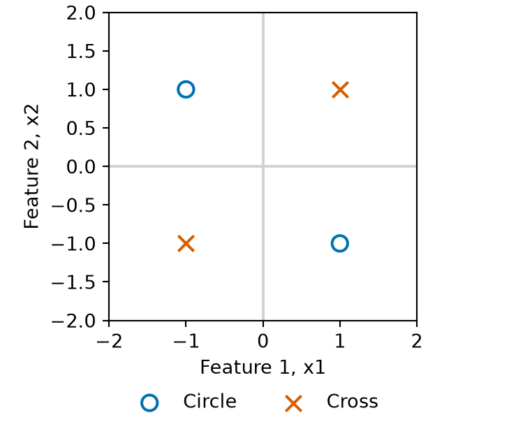
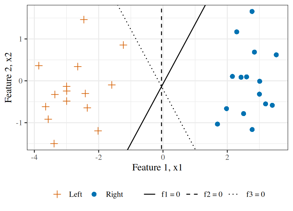
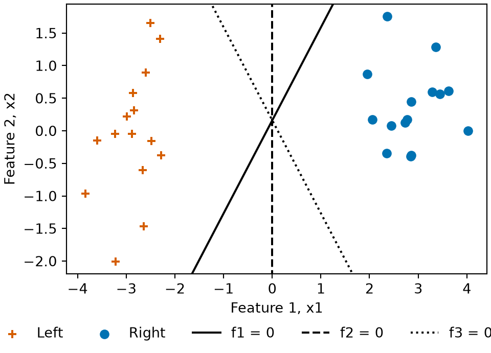
A colleague says logistic regression is “a linear model, so it can only draw straight boundaries, which makes it useless for the data in Figure 12”. The first clause is true and the conclusion does not follow. Explain why, and say what you would do to the features to separate those points.

SolutionSolution 27

Solution 27. The boundary is linear in the features, not in the raw measurements. Those coincide only when no nonlinear features are constructed from the measurements.

For Figure 12, the classes are separated by the sign of \(x_1 x_2\), so adding a third feature \(x_3 = x_1 x_2\) makes the data linearly separable in the three-dimensional feature space — the plane \(x_3 = 0\) separates the classes — while its intersection with the \((x_1, x_2)\) plane is the pair of coordinate axes, which no single line in two dimensions can represent.

This is the same construction linear regression uses when fitting a polynomial, and that neural networks automate by learning feature transformations from data.

ExrExercise 28 (The boundary is a hyperplane (part 5))

Exercise 28 (The boundary is a hyperplane (part 5)) Use the setup of Exercise 24.

Logistic regression and linear regression are both linear in \(\dprod{\vcoef}{\vx}\). State what is linear in each, and say which of the two has a linear relationship between features and the quantity actually reported.

SolutionSolution 28

Solution 28. In linear regression the prediction itself is linear in the features: \(\hy = \dprod{\vcoef}{\vx}\), and that is the number reported.

In logistic regression the log odds are linear in the features (Exercise 19), and the number reported is \(\sigmoid\) of that — which is not linear in anything.

So only linear regression has a linear relationship between features and the reported quantity. Calling logistic regression a linear model is a statement about its boundary and its log odds, and readers often misread it as a claim about its predictions.

LemTheorem 7 (The logistic regression boundary is a hyperplane)

Theorem 7 (The logistic regression boundary is a hyperplane) Let \(\coef{0}\) be the intercept and \(\vcoef \ne \vzero\) the vector of slopes of a logistic regression model. At threshold \(\thresh \in (0, 1)\), the decision boundary of the model is the hyperplane

\[ \coef{0} + \dprod{\vcoef}{\vpredvar} = \log \frac{\thresh}{1 - \thresh} \]

with normal vector \(\vcoef\). Changing the threshold translates the hyperplane and does not rotate it.

ProofProof

Proof. By Solution 24 to Solution 26.

ExmExample 13 (Moving the threshold)

Example 13 (Moving the threshold) For the model of Example 12, a threshold of \(\thresh = 0.9\) puts the boundary at \(-1 + 2 \predvar_1 + \predvar_2 = \log(0.9 / 0.1) = 2.197\). That is the same line, shifted by \(2.197 / \norm{\vcoef} = 0.983\) units along the normal vector \(\vcoef = (2, 1)\), in the direction that shrinks the region predicted \(1\).

library(ggplot2)
hb_coef <- c(-1, 2, 1)
hb_lines <- data.frame(
  threshold = c("0.5", "0.9"),
  intercept = (log(c(0.5, 0.9) / (1 - c(0.5, 0.9))) - hb_coef[1]) / hb_coef[3],
  slope = -hb_coef[2] / hb_coef[3]
)
hb_points <- data.frame(x1 = c(1, 0), x2 = c(1, 0), point = c("(1, 1)", "(0, 0)"))
ggplot() +
  geom_abline(
    data = hb_lines,
    aes(intercept = intercept, slope = slope, colour = threshold, linetype = threshold)
  ) +
  geom_point(data = hb_points, aes(x1, x2, shape = point), size = 3) +
  scale_colour_manual(values = c("0.5" = "#0072B2", "0.9" = "#D55E00")) +
  scale_shape_manual(values = c("(1, 1)" = 16, "(0, 0)" = 15)) +
  coord_cartesian(xlim = c(-1, 2), ylim = c(-2, 3)) +
  labs(
    x = "First feature", y = "Second feature",
    colour = "Threshold", linetype = "Threshold", shape = "Point"
  )

import matplotlib.pyplot as plt
import numpy as np

coef_hb = np.array([-1, 2, 1])
x1_hb = np.array([-1, 2])
fig, ax = plt.subplots(figsize=(5, 4), layout="constrained")
for threshold, colour, style in [(0.5, "#0072B2", "-"), (0.9, "#D55E00", "--")]:
    x2_hb = (np.log(threshold / (1 - threshold)) - coef_hb[0] - coef_hb[1] * x1_hb) / coef_hb[2]
    ax.plot(x1_hb, x2_hb, color=colour, linestyle=style, label=f"threshold {threshold}");
ax.plot(1, 1, color="black", marker="o", markersize=8, linestyle="", label="(1, 1)");
ax.plot(0, 0, color="black", marker="s", markersize=8, linestyle="", label="(0, 0)");
ax.set_xlim(-1, 2);
ax.set_ylim(-2, 3);
ax.set_xlabel("First feature");
ax.set_ylabel("Second feature");
fig.legend(loc="outside lower center", ncol=2);
plt.show()

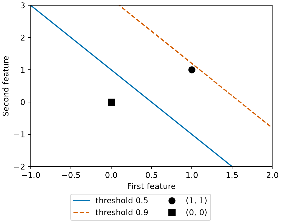
Figure 13: The decision boundary of Example 12 for the threshold \(0.5\) (solid) and the shifted boundary of Example 13 for \(0.9\) (dashed), with the two points of the first example. Raising the threshold moves the boundary up and shrinks the region of class \(1\), so the point \((1, 1)\) falls out of it.

R

(a)

Python

(b)

5 Fitting: where the cost comes from

The form of the model is specified, and the parameter vector \(\vcoef\) remains to be estimated. Logistic regression is a probability model, so maximum likelihood provides a criterion for choosing \(\vcoef\): the value that makes the observed labels most probable.

Maximum likelihood determines the loss function directly. Exercise 29, Exercise 30, and Exercise 31 derive the resulting log loss, and Exercise 32 and Exercise 33 show why squared-error loss on the probabilities is unsuitable.

ExrExercise 29 (Probability of a binary outcome in one formula)

Exercise 29 (Probability of a binary outcome in one formula) Exercise 19 specified the model: \(\Pr[Y = 1 \mid \vx] = \sigmoidf{\dprod{\vcoef}{\vx}}\). It did not specify how to estimate \(\vcoef\). Let \(\prob_i = \sigmoidf{\dprod{\vcoef}{\vx_i}}\) be the probability that the model assigns to observation \(i\) having label \(1\).

Express \(\Pr[Y_i = y_i \mid \vx_i]\) as a single formula that holds for both \(y_i = 0\) and \(y_i = 1\), and check it at each value.

SolutionSolution 29

Solution 29. \[\Pr[Y_i = y_i \mid \vx_i] = \prob_i^{y_i}\paren{1 - \prob_i}^{1 - y_i}\]

At \(y_i = 1\), the second factor is \((1-\prob_i)^0 = 1\) and the expression reads \(\prob_i\). At \(y_i = 0\), the first factor is \(\prob_i^0 = 1\) and the expression reads \(1 - \prob_i\). Each is the model’s assertion, so the single expression covers both cases.

The exponents select the factor corresponding to the observed outcome: each exponent is either \(0\) or \(1\), so one factor equals \(1\) and the other remains.

LemLemma 1 (Probability mass of one Bernoulli outcome)

Lemma 1 (Probability mass of one Bernoulli outcome) If \(\Outvar_i \mid \vpredvar_i \sim \Bernoulli\paren{\prob_i}\) and \(\outvar_i \in \set{0, 1}\), then

\[\Prf{\Outvar_i = \outvar_i \given \vpredvar_i} = \prob_i^{\outvar_i}\paren{1 - \prob_i}^{1 - \outvar_i}.\]

ProofProof

Proof. By Solution 29.

ExmExample 14 (The probability mass of one outcome)

Example 14 (The probability mass of one outcome) Take \(\prob_i = 0.8\). Lemma 1 gives the probabilities of the two outcomes, which match R’s dbinom:

p_bpmf <- 0.8
c(p_bpmf^1 * (1 - p_bpmf)^0, p_bpmf^0 * (1 - p_bpmf)^1)

[1] 0.8 0.2

dbinom(c(1, 0), size = 1, prob = p_bpmf)

[1] 0.8 0.2

ExrExercise 30 (Likelihood of the dataset)

Exercise 30 (Likelihood of the dataset) Using the single-observation probability from Exercise 29, express the likelihood \(L(\vcoef)\) of the full dataset in terms of the \(\prob_i = \sigmoidf{\dprod{\vcoef}{\vx_i}}\) and labels \(y_i\), and state the assumption required.

SolutionSolution 30

Solution 30. \[L(\vcoef) = \prodin \prob_i^{y_i}\paren{1 - \prob_i}^{1 - y_i}, \qquad \prob_i = \sigmoidf{\dprod{\vcoef}{\vx_i}}\]

Multiplying requires that the observations be conditionally independent given their features. Conditional independence is weaker than marginal independence of the \(Y_i\) — two patients from the same household may have correlated outcomes — but it rules out datasets in which \(y_1\) carries information about \(y_2\) beyond what \(\vx_2\) provides. Repeated measurements on the same subject, or students within a classroom, violate conditional independence and require a model with a shared random effect or cluster term.

LemLemma 2 (Likelihood of conditionally independent Bernoulli outcomes)

Lemma 2 (Likelihood of conditionally independent Bernoulli outcomes) If \(\Outvar_1, \dots, \Outvar_n\) are conditionally independent given \(\vpredvar_1, \dots, \vpredvar_n\) with \(\Outvar_i \mid \vpredvar_i \sim \Bernoulli\paren{\prob_i}\), where \(\prob_i\) is determined by the coefficients \(\vcoef\) and the observed outcomes are \(\outvar_i \in \set{0, 1}\), the likelihood is

\[L(\vcoef) = \prodin \prob_i^{\outvar_i}\paren{1 - \prob_i}^{1 - \outvar_i}.\]

ProofProof

Proof. By Solution 30.

ExmExample 15 (The likelihood of three outcomes)

Example 15 (The likelihood of three outcomes) Take the outcomes \((1, 0, 1)\) with \((\prob_1, \prob_2, \prob_3) = (0.9, 0.2, 0.7)\). Lemma 2 gives the product of the three probability masses:

y_bl <- c(1, 0, 1)
p_bl <- c(0.9, 0.2, 0.7)
prod(p_bl^y_bl * (1 - p_bl)^(1 - y_bl))

[1] 0.504

ExrExercise 31 (Log-likelihood of the dataset)

Exercise 31 (Log-likelihood of the dataset) Take the logarithm of the likelihood \(L(\vcoef)\) from Exercise 30 and simplify. Give two reasons to work with the log-likelihood \(\log L(\vcoef)\) rather than \(L(\vcoef)\).

SolutionSolution 31

Solution 31. \[ \begin{aligned} \llik(\vcoef) &= \log L(\vcoef) && \text{(definition of log-likelihood)} \\ &= \log\paren{\prodin \prob_i^{y_i}\paren{1 - \prob_i}^{1 - y_i}} && \text{(by @sol-bernoulli-likelihood)} \\ &= \sumin \log\paren{\prob_i^{y_i}\paren{1 - \prob_i}^{1 - y_i}} && \text{(log of a product)} \\ &= \sumin\sb{\log\paren{\prob_i^{y_i}} + \log\paren{\paren{1 - \prob_i}^{1 - y_i}}} && \text{(log of a product)} \\ &= \sumin\sb{y_i \log \prob_i + (1-y_i)\log\paren{1 - \prob_i}} && \text{(log of a power)} \end{aligned} \]

Two reasons.

Arithmetic. \(L(\vcoef)\) is a product of \(n\) numbers each below \(1\), so for \(n\) in the thousands it underflows to \(0\) in floating point and every candidate \(\vcoef\) evaluates to \(0\). The logarithm turns the product into a sum of terms of moderate magnitude.

Optimization. \(\log\) is strictly increasing, so it preserves the maximizer, and a sum differentiates term by term: the gradient of \(\llik(\vcoef)\) is the sum of \(n\) per-observation gradients, which simplifies Exercise 48 and enables stochastic gradient descent.

Maximizing \(\llik(\vcoef)\) is equivalent to minimizing \(-\llik(\vcoef)\), which is called the log loss or cross-entropy loss. The two names describe the same function, and no additional assumption is introduced: the log loss is the plausible loss under conditionally independent Bernoulli outcomes (Theorem 8).

LemLemma 3 (Log-likelihood of conditionally independent Bernoulli outcomes)

Lemma 3 (Log-likelihood of conditionally independent Bernoulli outcomes) Under the assumptions of Lemma 2, the log-likelihood is

\[\llik(\vcoef) = \sumin\sb{\outvar_i \log \prob_i + (1-\outvar_i)\log\paren{1 - \prob_i}}.\]

ProofProof

Proof. By Solution 31.

ExmExample 16 (The log-likelihood of three outcomes)

Example 16 (The log-likelihood of three outcomes) With the outcomes and probabilities of Example 15, Lemma 3 gives the log-likelihood as a sum, which equals the log of the likelihood:

y_bll <- c(1, 0, 1)
p_bll <- c(0.9, 0.2, 0.7)
sum(y_bll * log(p_bll) + (1 - y_bll) * log(1 - p_bll))

[1] -0.685179

log(prod(p_bll^y_bll * (1 - p_bll)^(1 - y_bll)))

[1] -0.685179

ExrExercise 32 (Negative log-likelihood on a positive observation)

Exercise 32 (Negative log-likelihood on a positive observation) Consider one observation with label \(y_i = 1\) in the log-likelihood of Exercise 31. Give its contribution to \(-\log L(\vcoef)\) at \(\prob_i = 0.9\), \(0.5\), \(0.1\), and \(0.01\), to three significant figures, and state what happens as \(\prob_i \to 0\).

SolutionSolution 32

Solution 32. With \(y_i = 1\), observation \(i\)’s contribution to \(-\log L(\vcoef)\) is \(-\log \prob_i\):

\(\prob_i\)	\(-\log \prob_i\)
\(0.9\)	\(0.105\)
\(0.5\)	\(0.693\)
\(0.1\)	\(2.30\)
\(0.01\)	\(4.61\)

As \(\prob_i \to 0\), the loss grows without bound. Assigning probability \(0\) to an outcome that occurs gives an infinite loss; the loss is unbounded above even though the predicted probability is in \((0,1)\).

ExrExercise 33 (Why squared error on the probabilities is unsuitable)

Exercise 33 (Why squared error on the probabilities is unsuitable) Under squared-error loss, the positive observation of Exercise 32 contributes \((\prob_i - y_i)^2\), which never exceeds \(1\) regardless of how small \(\prob_i\) is. Explain what that upper bound allows a fitted model to do without incurring a large loss, and state which of the two requirements in Exercise 4 the log loss satisfies.

SolutionSolution 33

Solution 33. Because the squared-error loss on a single observation is at most \(1\), the loss on one misclassified observation is bounded above by \(1\) even as \(\prob_i \to 0\). If allowing \(\prob_i \to 0\) on one observation with \(y_i = 1\) reduces the sum of squared errors across the remaining observations by more than \(1\), the total squared error decreases. Under the log loss, \(-\log \prob_i \to \infty\) as \(\prob_i \to 0\) (Solution 32), so no finite reduction in loss on the remaining observations can offset assigning \(\prob_i \to 0\) to an observation with \(y_i = 1\).

This unbounded penalty satisfies the second requirement of Exercise 4. The loss saturates on the correct side — \(-\log \prob_i\) approaches \(0\) with vanishing derivative as \(\prob_i \to 1\), so increasing the margin on an already well-classified observation reduces the loss by very little — and grows without bound on the wrong side.

One caveat: we should not overstate the argument. Squared error on a probability is the Brier score, and it is a proper scoring rule: its expected value is minimized by reporting the true probability, exactly as the log loss’s is. So the case against squared error here is not that it rewards dishonesty. Squared error has three faults instead: the boundedness above; the loss of the maximum-likelihood reading, which supplies standard errors and likelihood ratio tests for the fitted coefficients; and the vanishing gradient that Exercise 48 exhibits. Squared error on \(\prob_i\) is neither a plausible loss for Bernoulli outcomes nor a friendly loss when paired with the logistic function, whereas the log loss is both.

DefDefinition 3 (Cross-entropy loss (also called log loss))

Definition 3 (Cross-entropy loss (also called log loss)) For a label \(\outvar_i \in \set{0, 1}\) and a predicted probability \(\prob_i = \Prf{\Outvar_i = 1 \mid \vpredvar_i}\), the per-observation cross-entropy loss, also called the log loss, is

\[ \begin{aligned} \lossf{\outvar_i, \prob_i} &= C_i \\ &= -\outvar_i \log \prob_i - (1 - \outvar_i) \log (1 - \prob_i). \end{aligned} \]

Summed over the \(n\) observations, the total log loss is the negative log-likelihood of conditionally independent Bernoulli labels (Solution 31),

\[ \begin{aligned} C(\vcoef) &= \sumin C_i \\ &= \sumin \sb{ -\outvar_i \log \prob_i - (1 - \outvar_i) \log (1 - \prob_i) } \\ &= -\llik(\vcoef), \end{aligned} \]

and its average \(\empriskf{\vcoef} = \tfrac{1}{n} C(\vcoef)\) is the empirical risk. Different sources apply the name log loss or cross-entropy loss to the per-observation loss function \(\lossf{\outvar_i, \prob_i}\), to the sum \(C(\vcoef)\), or to the average \(\empriskf{\vcoef}\) [15].

ExmExample 17 (Log loss and squared error on a positive case)

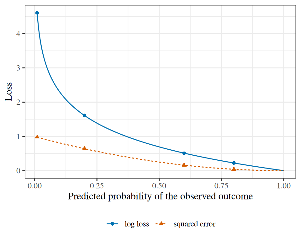
Example 17 (Log loss and squared error on a positive case) For an observation with \(\outvar_i = 1\), evaluate the log loss \(C_i = -\log \prob_i\) and the squared error \((\prob_i - \outvar_i)^2\) across \(\prob_i = 0.8, 0.6, 0.2, 0.01\):

R

prob_ll <- c(0.8, 0.6, 0.2, 0.01)
log_loss_ll <- -log(prob_ll)
sq_err_ll <- (prob_ll - 1)^2
round(
  data.frame(prob = prob_ll, log_loss = log_loss_ll, squared_error = sq_err_ll),
  3
)

Python

import numpy as np
import pandas as pd

prob_ll = np.array([0.8, 0.6, 0.2, 0.01])
print(pd.DataFrame({
    "prob": prob_ll,
    "log_loss": -np.log(prob_ll),
    "squared_error": (prob_ll - 1.0) ** 2,
}).round(3))

   prob  log_loss  squared_error
0  0.80     0.223           0.04
1  0.60     0.511           0.16
2  0.20     1.609           0.64
3  0.01     4.605           0.98

At \(\prob_i = 0.8\), both losses are small (0.223 and 0.04). At \(\prob_i = 0.01\), squared error reaches 0.98, just below its ceiling of \(1\), while the log loss reaches 4.61 and grows without bound as \(\prob_i \to 0\).

library(ggplot2)
ll_curve <- data.frame(prob = seq(0.01, 1, length.out = 300))
ll_long <- data.frame(
  prob = rep(ll_curve$prob, 2),
  loss = c(-log(ll_curve$prob), (ll_curve$prob - 1)^2),
  kind = rep(c("log loss", "squared error"), each = nrow(ll_curve))
)
ll_points <- data.frame(
  prob = rep(prob_ll, 2),
  loss = c(log_loss_ll, sq_err_ll),
  kind = rep(c("log loss", "squared error"), each = length(prob_ll))
)
ggplot(ll_long, aes(prob, loss, colour = kind, linetype = kind)) +
  geom_line() +
  geom_point(aes(shape = kind), data = ll_points) +
  scale_colour_manual(values = c("log loss" = "#0072B2", "squared error" = "#D55E00")) +
  labs(x = "Predicted probability of the observed outcome", y = "Loss", colour = NULL, linetype = NULL, shape = NULL)

import matplotlib.pyplot as plt
import numpy as np

p_ll = np.linspace(0.01, 1, 300)
fig, ax = plt.subplots(figsize=(5, 4), layout="constrained")
ax.plot(p_ll, -np.log(p_ll), color="#0072B2", linestyle="-", label="log loss");
ax.plot(p_ll, (p_ll - 1) ** 2, color="#D55E00", linestyle="--", label="squared error");
ax.plot(prob_ll, -np.log(prob_ll), color="#0072B2", marker="o", linestyle="");
ax.plot(prob_ll, (prob_ll - 1) ** 2, color="#D55E00", marker="^", linestyle="");
ax.set_xlabel("Predicted probability of the observed outcome");
ax.set_ylabel("Loss");
fig.legend(loc="outside lower center", ncol=2);
plt.show()

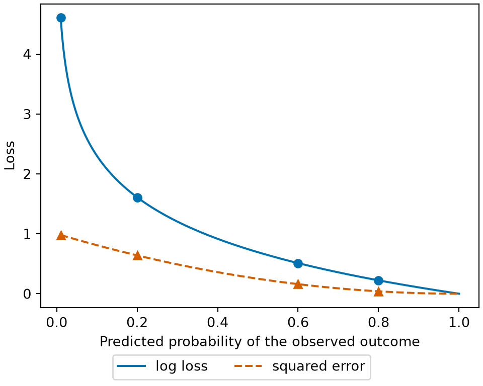
Figure 14: The log loss and the squared error of Example 17 for a positive case, as the probability given to the positive class moves from 0 to 1, with the four values of the example marked. The squared error stays below 1, while the log loss grows without bound as the probability approaches 0.

R

(a)

Python

(b)

LemTheorem 8 (Minimizing the log loss is maximum likelihood estimation)

Theorem 8 (Minimizing the log loss is maximum likelihood estimation) Suppose the outcomes \(\Outvar_1, \dots, \Outvar_n \in \set{0, 1}\) are conditionally independent given \(\vpredvar_1, \dots, \vpredvar_n\), with

\[ \Outvar_i \mid \vpredvar_i \sim \Bernoulli\paren{\prob_i}, \qquad \prob_i = \sigmoidf{\dprod{\vcoef}{\vpredvar_i}}. \]

Then minimizing the total log loss \(C(\vcoef)\) (or the empirical risk \(\empriskf{\vcoef} = \tfrac{1}{n} C(\vcoef)\)) with respect to \(\vcoef\) yields the maximum likelihood estimate \(\hvcoef\). The log loss is therefore the plausible loss for conditionally independent Bernoulli outcomes.

ProofProof

Proof. By assumption, the outcomes are conditionally independent with \(\Outvar_i \mid \vpredvar_i \sim \Bernoulli\paren{\prob_i}\), so Lemma 2 gives the likelihood and Lemma 3 gives the log-likelihood \(\llik(\vcoef)\), which is \(-C(\vcoef)\) by the definition of the log loss. Because \(\log\) is strictly increasing and \(n > 0\), maximizing the likelihood is equivalent to maximizing \(\llik(\vcoef)\), which is equivalent to minimizing \(C(\vcoef)\) or \(\tfrac{1}{n} C(\vcoef)\).

ExmExample 18 (Minimizing the log loss on the WCGS data recovers the maximum likelihood fit)

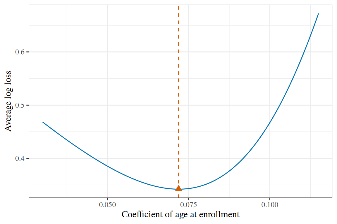
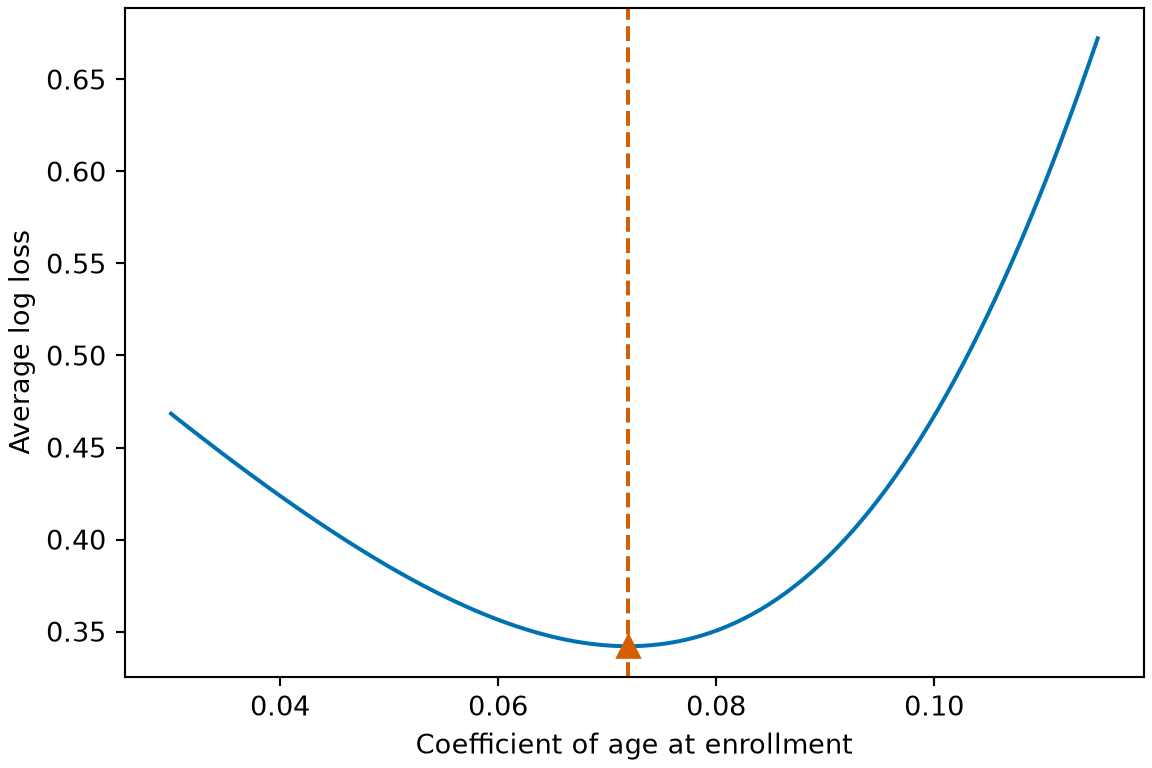
Example 18 (Minimizing the log loss on the WCGS data recovers the maximum likelihood fit) Take the WCGS data of Exercise 1 (data/wcgs.csv), whose column dibpat records each man’s behavior pattern, type A or type B. Subset to the men of type A (dibpat is "A"), so that a single curve with two coefficients describes them. Model coronary heart disease (chd) on age at enrollment (age) with \(\prob_i = \sigmoidf{\coef{0} + \coef{1}\,\text{age}_i}\). Minimize the average log loss (empirical risk) \(\empriskf{\vcoef} = \tfrac{1}{n} C(\vcoef)\) numerically from \(\vcoef = \vzero\), and compare with the maximum likelihood fit:

R

wcgs_mle <- subset(read.csv("data/wcgs.csv"), dibpat == "A")
y_wcgs <- wcgs_mle$chd
x_wcgs <- cbind(1, wcgs_mle$age)

mean_log_loss <- function(b) {
  p <- plogis(drop(x_wcgs %*% b))
  mean(-y_wcgs * log(p) - (1 - y_wcgs) * log(1 - p))
}

loss_fit <- optim(c(0, 0), mean_log_loss, control = list(reltol = 1e-14))
glm_fit <- coef(glm(chd ~ age, family = binomial, data = wcgs_mle))
round(rbind(log_loss_minimizer = loss_fit$par, mle = unname(glm_fit)), 6)

                        [,1]     [,2]
log_loss_minimizer -5.498861 0.071907
mle                -5.498862 0.071907

Python

import numpy as np
import pandas as pd
import statsmodels.api as sm
from scipy.optimize import minimize
from scipy.special import expit

wcgs_all = pd.read_csv("data/wcgs.csv")
wcgs_mle = wcgs_all[wcgs_all["dibpat"] == "A"]
y_wcgs = wcgs_mle["chd"].to_numpy(float)
x_wcgs = sm.add_constant(wcgs_mle["age"].to_numpy(float))

def mean_log_loss(b):
    p = expit(x_wcgs @ b)
    return np.mean(-y_wcgs * np.log(p) - (1.0 - y_wcgs) * np.log(1.0 - p))

loss_fit = minimize(
    mean_log_loss,
    x0=np.zeros(2),
    method="Nelder-Mead",
    options={"xatol": 1e-10, "fatol": 1e-14},
)
glm_fit = sm.GLM(y_wcgs, x_wcgs, family=sm.families.Binomial()).fit().params
print(pd.DataFrame({"intercept": [loss_fit.x[0], glm_fit[0]],
                    "age": [loss_fit.x[1], glm_fit[1]]},
                   index=["log_loss_minimizer", "mle"]).round(6))

                    intercept       age
log_loss_minimizer  -5.498862  0.071907
mle                 -5.498862  0.071907

The numerical minimizer of \(\empriskf{\vcoef}\) and the maximum likelihood estimate agree to within 3.4e-07, as Theorem 8 states.

library(ggplot2)
llm_slopes <- seq(0.03, 0.115, length.out = 111)
llm_curve <- data.frame(
  slope = llm_slopes,
  loss = vapply(llm_slopes, \(s) mean_log_loss(c(glm_fit[[1]], s)), numeric(1))
)
llm_pt <- data.frame(slope = loss_fit$par[2], loss = mean_log_loss(loss_fit$par))
ggplot(llm_curve, aes(slope, loss)) +
  geom_line(colour = "#0072B2") +
  geom_vline(xintercept = glm_fit[[2]], linetype = "dashed", colour = "#D55E00") +
  geom_point(data = llm_pt, colour = "#D55E00", shape = 17, size = 3) +
  labs(x = "Coefficient of age at enrollment", y = "Average log loss")

import matplotlib.pyplot as plt
import numpy as np

slopes_llm = np.linspace(0.03, 0.115, 111)
loss_llm = [mean_log_loss(np.array([glm_fit[0], s])) for s in slopes_llm]
fig, ax = plt.subplots(figsize=(6, 4), layout="constrained")
ax.plot(slopes_llm, loss_llm, color="#0072B2");
ax.axvline(glm_fit[1], color="#D55E00", linestyle="--");
ax.plot(loss_fit.x[1], mean_log_loss(loss_fit.x), color="#D55E00", marker="^", markersize=8,
        linestyle="");
ax.set_xlabel("Coefficient of age at enrollment");
ax.set_ylabel("Average log loss");
plt.show()

Figure 15: The average log loss of Example 18, for the type A men, as the coefficient of age at enrollment varies, with the intercept held at its fitted value. The numerical minimizer (triangle) and the maximum likelihood coefficient (dashed line) coincide.

R

(a)

Python

(b)

ExrExercise 34 (The same loss, written two ways)

Exercise 34 (The same loss, written two ways) Exercise 31 wrote the per-observation cost with labels \(y \in \{0, 1\}\):

\[C(\logodds, y) = -y\log\sigmoid(\logodds) - (1-y)\log\paren{1 - \sigmoid(\logodds)}, \qquad \logodds = \dprod{\vcoef}{\vx}\]

Much of the literature instead uses \(\tilde y \in \{-1, +1\}\), via \(\tilde y = 2y - 1\).

Show that \(C(\logodds, \outvar) = \log\paren{1 + \e{-\tilde \outvar \logodds}}\).

SolutionSolution 34

Solution 34. We check the two cases \(y = 1\) and \(y = 0\) separately.

If \(y = 1\), then \(\tilde y = +1\) and the second term of \(C\) vanishes:

\[ \begin{aligned} C &= -\log\sigmoid(\logodds) \\ &= -\log\frac{1}{1 + e^{-\logodds}} \\ &= \log\paren{1 + e^{-\logodds}} \\ &= \log\paren{1 + e^{-\tilde y \logodds}} \end{aligned} \]

If \(y = 0\), then \(\tilde y = -1\) and the first term vanishes. Using \(1 - \sigmoid(\logodds) = \sigmoid(-\logodds)\) from Exercise 8 gives

\[ \begin{aligned} C &= -\log\paren{1 - \sigmoid(\logodds)} \\ &= -\log\sigmoid(-\logodds) \\ &= \log\paren{1 + e^{\logodds}} \\ &= \log\paren{1 + e^{-\tilde y \logodds}} \end{aligned} \]

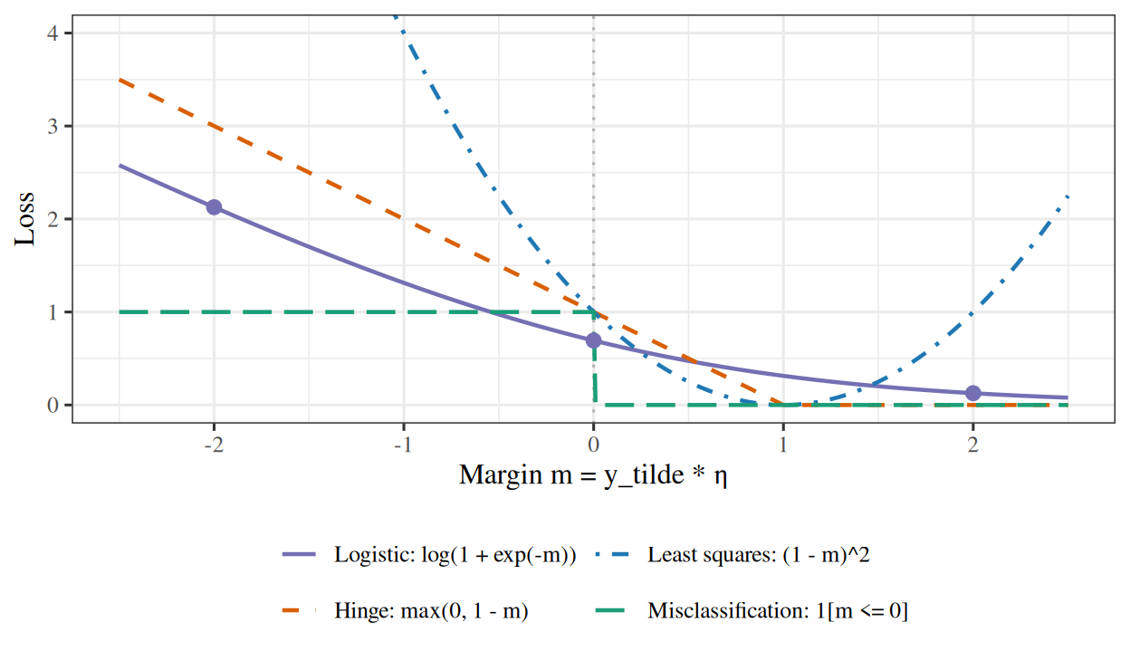
Both cases yield the same expression, so the two formulas represent the same loss function under the two label conventions. Under the \(\{-1, +1\}\) convention, the loss depends on \(\logodds\) and \(\tilde y\) only through their product \(m = \tilde y \logodds\). The margin \(m\) is positive if and only if the observation is on the correct side of the decision boundary of Exercise 24, and \(\abs{m}\) measures how far the score is from the boundary.

ExrExercise 35 (The same loss, written two ways (part 2))

Exercise 35 (The same loss, written two ways (part 2)) Use the setup of Exercise 34.

Let \(m = \tilde \outvar \logodds\) be the margin. Describe \(\log(1 + \e{-m})\) as a function of \(m\): its monotonicity, its value at \(m = 0\), and its behaviour as \(m \to +\infty\) and as \(m \to -\infty\). Give the value at \(m = 0\) and at \(m = \pm 2\) to three significant figures.

SolutionSolution 35

Solution 35. The function \(\log(1 + e^{-m})\) is strictly decreasing in \(m\) because \(e^{-m}\) is strictly decreasing. Larger margins therefore always yield smaller loss, and the loss orders observations by their signed margin.

\(m\)	\(\log(1 + e^{-m})\)
\(-2\)	\(2.13\)
\(0\)	\(0.693\)
\(+2\)	\(0.127\)

At \(m = 0\) the loss is \(\log 2 \approx 0.693\), which is the log loss of predicting probability \(\tfrac12\) for both classes.

As \(m \to +\infty\), the loss approaches \(0\) but remains strictly positive for every finite \(m\). Increasing the margin of an already correctly classified observation always reduces the loss slightly, which leads to the divergence under linear separation analyzed in Exercise 92.

As \(m \to -\infty\), \(\log(1 + e^{-m}) \approx \log e^{-m} = -m\), so the loss grows linearly with the magnitude of a negative margin, whereas squared error grows quadratically. A single severely misclassified observation therefore has bounded influence on the gradient under logistic loss, unlike under squared error, as seen in Exercise 3.

Comparing the derivatives with respect to \(\logodds\) makes this difference explicit. Fitting a linear predictor \(\logodds\) to \(\tilde y \in \{-1, +1\}\) by least squares uses the loss \((\tilde y - \logodds)^2 = (1 - m)^2\), whose derivative with respect to \(\logodds\) is \(2(\logodds - \tilde y)\), whereas the derivative of the logistic loss is \(-\tilde y\,\sigmoid(-m)\). Suppose \(\tilde y = +1\):

• At \(\logodds = -4\) (a confidently wrong prediction), the logistic derivative is \(-\sigmoid(4) \approx -0.98\), whereas the least-squares derivative is \(2(-4 - 1) = -10\).
• At \(\logodds = 4\) (a confidently correct prediction), the logistic derivative is \(-\sigmoid(-4) \approx -0.02\), which is near \(0\), whereas the least-squares derivative is \(2(4 - 1) = 6\).

Squared error continues to penalize predictions with \(\logodds = 4 > 1\) because \(\logodds \ne \tilde y\), and places large weight on observations with large negative margins. The logistic loss avoids both behaviors. Figure 16 plots the logistic, hinge, squared-error, and zero–one misclassification losses as functions of the margin \(m\).

ExrExercise 36 (The same loss, written two ways (part 3))

Exercise 36 (The same loss, written two ways (part 3)) Use the setup of Exercise 34.

Compare the logistic loss with the hinge loss \(\max(0,\, 1 - m)\), which support vector machines use. State one property that the hinge loss has and the logistic loss does not, and one property that the logistic loss has and the hinge loss does not.

SolutionSolution 36

Solution 36. The hinge loss \(\max(0, 1 - m)\) is identically \(0\) for all \(m \ge 1\). Observations with margin greater than \(1\) contribute zero gradient, so the fitted decision boundary of a support vector machine depends only on the observations with \(m \le 1\) (the support vectors). In contrast, the logistic loss is strictly positive for all finite \(m\), so every observation contributes to the fit, with weight decreasing exponentially as \(m \to +\infty\).

Conversely, the logistic loss is smooth everywhere, whereas the hinge loss has a corner at \(m = 1\) where it is not differentiable, requiring subgradient methods or constrained quadratic programming. Moreover, because the logistic loss is the negative log-likelihood of a Bernoulli model, minimizing it produces calibrated probability estimates \(\sigmoid(\logodds)\), whereas a support vector machine produces an uncalibrated score whose conversion to a probability requires an additional post-processing step.

ExrExercise 37 (The same loss, written two ways (part 4))

Exercise 37 (The same loss, written two ways (part 4)) Use the setup of Exercise 34.

What we actually care about is the misclassification rate, whose per-observation cost is \(\mathbb{1}[m \le 0]\). Say why it is not used for fitting. Then show that \[\mathbb{1}[m \le 0] \;\le\; \frac{1}{\log 2}\,\log\paren{1 + e^{-m}} \quad\text{for every } m\] and say what reducing the right-hand side therefore gains.

SolutionSolution 37

Solution 37. The zero–one misclassification loss \(\truthind(m \le 0)\) is piecewise constant: its derivative with respect to \(\vcoef\) is zero wherever it is differentiable and undefined at \(m = 0\), so gradient-based optimizers receive no directional signal. It is also non-convex, and minimizing the number of misclassified training points with a linear classifier is NP-hard in general.

To verify the upper bound \(\truthind(m \le 0) \le \log(1 + e^{-m}) / \log 2\), we check the two cases \(m \le 0\) and \(m > 0\):

• If \(m \le 0\), the left-hand side is \(1\), and since \(e^{-m} \ge 1\), we have \(\log(1 + e^{-m}) \ge \log 2\), so the right-hand side is at least \(\log 2 / \log 2 = 1\).
• If \(m > 0\), the left-hand side is \(0\), and the right-hand side is strictly positive because \(\log(1 + e^{-m}) > 0\) for every finite \(m\).

Thus the inequality holds for all \(m \in \reals\).

Averaging over the training set shows that the mean logistic loss divided by \(\log 2\) is an upper bound on the training misclassification rate. Minimizing the logistic loss therefore minimizes a smooth, convex surrogate upper bound on the zero–one error rate.

The bound is not tight for positive margins: at \(m = 2\), the rescaled logistic loss is \(0.127/\log 2 = 0.183\) even though the misclassification loss is \(0\), so a model can reduce its logistic loss by increasing positive margins without changing any classification decision.

LemTheorem 9 (The log loss depends on the margin alone)

Theorem 9 (The log loss depends on the margin alone) Let \(y \in \{0, 1\}\), \(\tilde y = 2y - 1 \in \{-1, +1\}\) and \(\logodds = \dprod{\vcoef}{\vx}\). Then the per-observation log loss,

\[ \lossf{y, \sigmoid(\logodds)} = -y\log\sigmoid(\logodds) - (1-y)\log\paren{1 - \sigmoid(\logodds)}, \]

equals \(\log\paren{1 + \e{-m}}\) with the margin \(m = \tilde y \logodds\). This loss is strictly decreasing in \(m\).

ProofProof

Proof. This is the solution to Exercise 34 and Exercise 35: see Solution 35.

ExmExample 19 (Evaluating the log loss from the score and from the margin)

Example 19 (Evaluating the log loss from the score and from the margin) Consider a linear score \(\logodds = 2\), so \(\prob = \sigmoid(2)\) is 0.881, and compare the log loss under the two labels \(y = 1\) (\(\tilde y = +1\), margin \(m = +2\)) and \(y = 0\) (\(\tilde y = -1\), margin \(m = -2\)):

R

z_mf <- 2
y_mf <- c(1, 0)
y_tilde_mf <- 2 * y_mf - 1
m_mf <- y_tilde_mf * z_mf
p_mf <- plogis(z_mf)

from_prob <- -y_mf * log(p_mf) - (1 - y_mf) * log(1 - p_mf)
from_margin <- log1p(exp(-m_mf))
round(data.frame(y = y_mf, y_tilde = y_tilde_mf, margin = m_mf,
                 from_prob = from_prob, from_margin = from_margin), 3)

Python

import numpy as np
import pandas as pd
from scipy.special import expit

z_mf = 2.0
y_mf = np.array([1, 0])
y_tilde_mf = 2 * y_mf - 1
m_mf = y_tilde_mf * z_mf
p_mf = expit(z_mf)

print(pd.DataFrame({
    "y": y_mf,
    "y_tilde": y_tilde_mf,
    "margin": m_mf,
    "from_prob": -y_mf * np.log(p_mf) - (1 - y_mf) * np.log(1 - p_mf),
    "from_margin": np.log1p(np.exp(-m_mf)),
}).round(3))

   y  y_tilde  margin  from_prob  from_margin
0  1        1     2.0      0.127        0.127
1  0       -1    -2.0      2.127        2.127

Both formulas return 0.127 on the correctly classified observation (\(m = +2\)) and 2.13 on the misclassified one (\(m = -2\)).

library(ggplot2)

m_grid <- seq(-2.5, 2.5, length.out = 501)
margin_df <- rbind(
  data.frame(
    m = m_grid,
    loss = log1p(exp(-m_grid)),
    kind = "Logistic: log(1 + exp(-m))"
  ),
  data.frame(
    m = m_grid,
    loss = pmax(0, 1 - m_grid),
    kind = "Hinge: max(0, 1 - m)"
  ),
  data.frame(
    m = m_grid,
    loss = (1 - m_grid)^2,
    kind = "Least squares: (1 - m)^2"
  ),
  data.frame(
    m = m_grid,
    loss = as.numeric(m_grid <= 0),
    kind = "Misclassification: 1[m <= 0]"
  )
)
margin_df$kind <- factor(
  margin_df$kind,
  levels = c(
    "Logistic: log(1 + exp(-m))",
    "Hinge: max(0, 1 - m)",
    "Least squares: (1 - m)^2",
    "Misclassification: 1[m <= 0]"
  )
)

logistic_pts <- data.frame(
  m = c(-2, 0, 2),
  loss = log1p(exp(-c(-2, 0, 2)))
)

ggplot(margin_df) +
  aes(m, loss, colour = kind, linetype = kind) +
  geom_vline(xintercept = 0, colour = "grey70", linetype = "dotted") +
  geom_line(linewidth = 0.8) +
  geom_point(
    data = logistic_pts,
    aes(m, loss),
    inherit.aes = FALSE,
    colour = "#7570b3",
    size = 2.4
  ) +
  scale_colour_manual(values = c(
    "Logistic: log(1 + exp(-m))" = "#7570b3",
    "Hinge: max(0, 1 - m)" = "#d95f02",
    "Least squares: (1 - m)^2" = "#1f78b4",
    "Misclassification: 1[m <= 0]" = "#1b9e77"
  )) +
  scale_linetype_manual(values = c(
    "Logistic: log(1 + exp(-m))" = "solid",
    "Hinge: max(0, 1 - m)" = "dashed",
    "Least squares: (1 - m)^2" = "dotdash",
    "Misclassification: 1[m <= 0]" = "longdash"
  )) +
  coord_cartesian(ylim = c(0, 4)) +
  guides(colour = guide_legend(nrow = 2), linetype = guide_legend(nrow = 2)) +
  labs(
    x = "Margin m = y_tilde * η",
    y = "Loss",
    colour = NULL,
    linetype = NULL
  ) +
  theme(legend.position = "bottom")

Figure 16: The log loss \(\log(1 + e^{-m})\), the hinge loss \(\max(0, 1 - m)\), the least-squares margin loss \((1 - m)^2\) and the misclassification loss \(\ind{m \le 0}\) as functions of the margin \(m = \tilde y \logodds\). Dots mark the three logistic-loss values tabulated in Solution 34: \((-2, 2.13)\), \((0, \log 2 \approx 0.693)\) and \((2, 0.127)\).

ExrExercise 38 (Three names for the same optimization)

Exercise 38 (Three names for the same optimization) The fit of Exercise 31 can be described three ways, and different fields use different ones.

Starting from \(\argmax_{\vcoef}\llik(\vcoef)\), derive the other two formulations: minimizing the negative log-likelihood, and empirical risk minimization \(\argmin_{\vcoef}\empriskf{\vcoef}\) with \(\emprisk = \tfrac1\nobs\sum_i \lossf{\outvar_i, \prob_i}\).

SolutionSolution 38

Solution 38. Maximizing \(\llik\) is minimizing \(-\llik\), and dividing by the positive constant \(n\) changes neither:

\[ \begin{aligned} \argmax_{\vcoef}\ \sum_i \sb{y_i\log\prob_i + (1-y_i)\log(1-\prob_i)} &= \argmin_{\vcoef}\ -\sum_i \sb{\cdots} \\ &= \argmin_{\vcoef}\ \frac1n \sum_i \lossf{y_i, \prob_i} \end{aligned} \]

ExrExercise 39 (Three names for the same optimization (part 2))

Exercise 39 (Three names for the same optimization (part 2)) Use the setup of Exercise 38.

State the per-observation loss \(\lossf{\outvar_i, \prob_i}\).

SolutionSolution 39

Solution 39. The per-observation loss is

\[\lossf{y, \prob} = -y\log\prob - (1-y)\log(1-\prob),\]

the log loss, also called the cross-entropy loss — Solution 42 says why.

ExrExercise 40 (Three names for the same optimization (part 3))

Exercise 40 (Three names for the same optimization (part 3)) Use the setup of Exercise 38.

Identify which step introduces the factor \(\tfrac1\nobs\).

SolutionSolution 40

Solution 40. The \(\tfrac1n\) enters at the last step and nowhere else.

ExrExercise 41 (Three names for the same optimization (part 4))

Exercise 41 (Three names for the same optimization (part 4)) Use the setup of Exercise 38.

State what the factor \(\tfrac1\nobs\) does and does not change, referring to Exercise 103.

SolutionSolution 41

Solution 41. It cannot move the minimizer, because scaling an objective by a positive constant leaves its argmin alone, and it cannot change the score equations, because those set a gradient to zero and zero scales to zero.

It does change every quantity that is not an argmin: the gradient’s size, and so any step size tuned against it; and the second derivative, and so any standard error computed from it. Exercise 103 is the same distinction seen from the opposite side, where a \(\tfrac1n\) had been attached to a log-likelihood that did not have one.

ExrExercise 42 (Three names for the same optimization (part 5))

Exercise 42 (Three names for the same optimization (part 5)) Use the setup of Exercise 38.

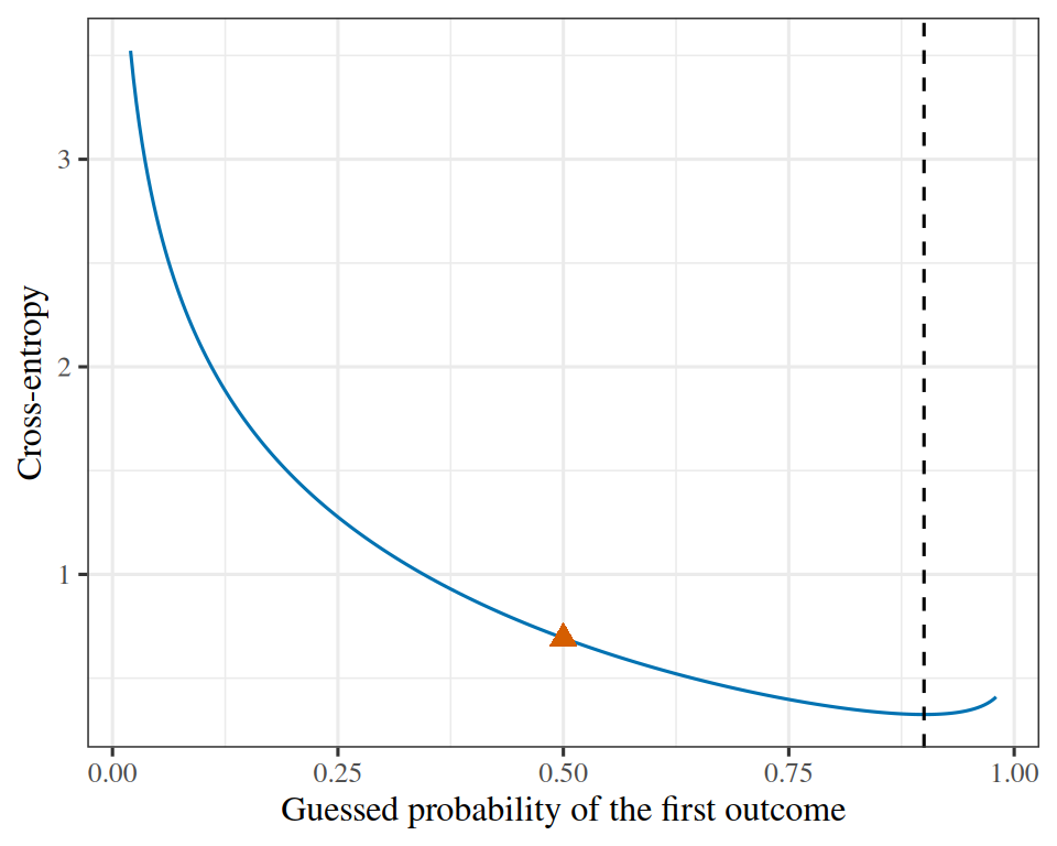
For distributions \(\vp\) and \(\vq\) over the same outcomes, the cross-entropy is \(H(\vp, \vq) = -\sum_j p_j \log q_j\). Let \(\vp = (1 - \outvar,\; \outvar)\) be the point-mass distribution at the observed label \(\outvar \in \{0, 1\}\), and let \(\vq = (1 - \prob,\; \prob)\). Show that \(H(\vp, \vq)\) equals the per-observation loss of Exercise 38.

SolutionSolution 42

Solution 42. The two distributions are over the two outcomes \(\{0, 1\}\), so the sum has two terms:

\[ \begin{aligned} H(\vp, \vq) &= -p_0\log q_0 - p_1 \log q_1 \\ &= -(1 - y)\log(1 - \prob) - y\log\prob, \end{aligned} \]

which is \(\lossf{y, \prob}\) exactly.

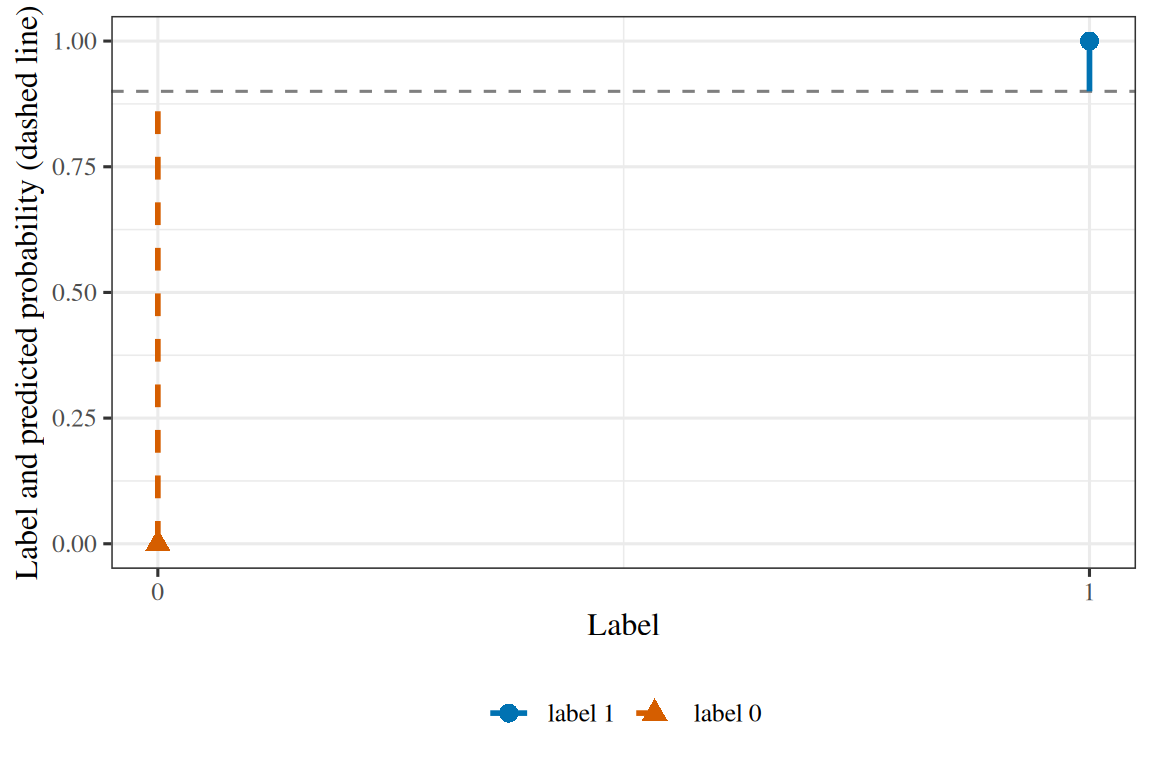
So the log loss is the cross-entropy between the label, read as a degenerate distribution putting all its mass on the observed outcome, and the distribution the model predicts. The three names in this exercise’s title are one calculation.

ExrExercise 43 (Three names for the same optimization (part 6))

Exercise 43 (Three names for the same optimization (part 6)) Use the setup of Exercise 38.

Show \(H(\vp, \vq) \ge H(\vp, \vp)\), with equality only when \(\vq = \vp\).

SolutionSolution 43

Solution 43. Subtract and collect:

\[ \begin{aligned} H(\vp, \vq) - H(\vp, \vp) &= \sum_j p_j \log\frac{p_j}{q_j} \\ &=: D_{\mathrm{KL}}(\vp \,\|\, \vq). \end{aligned} \]

This difference is the Kullback–Leibler divergence of \(\vq\) from \(\vp\).

Use \(\log x \le x - 1\), with equality only at \(x = 1\):

\[ \begin{aligned} -D_{\mathrm{KL}}(\vp\,\|\,\vq) &= \sum_j p_j \log\frac{q_j}{p_j} \\ &\le \sum_j p_j\paren{\frac{q_j}{p_j} - 1} \\ &= \sum_j q_j - \sum_j p_j \\ &= 1 - 1 \\ &= 0, \end{aligned} \]

so \(D_{\mathrm{KL}} \ge 0\) and \(H(\vp, \vq) \ge H(\vp, \vp)\). Equality needs \(q_j/p_j = 1\) wherever \(p_j > 0\), which for two distributions that both sum to one implies \(\vq = \vp\).

ExrExercise 44 (Three names for the same optimization (part 7))

Exercise 44 (Three names for the same optimization (part 7)) Use the setup of Exercise 38.

Evaluate \(H(\vp, \vp)\) for the \(\vp\) of Exercise 42.

SolutionSolution 44

Solution 44. Here \(\vp = (1-y, y)\) with \(y \in \{0,1\}\), so all its mass is on one outcome and

\[ \begin{aligned} H(\vp, \vp) &= -1\log 1 - 0\log 0 \\ &= 0, \end{aligned} \]

taking \(0\log 0 = 0\), its limit.

ExrExercise 45 (Three names for the same optimization (part 8))

Exercise 45 (Three names for the same optimization (part 8)) Use the setup of Exercise 38.

State the smallest achievable per-observation loss and when it is attained.

SolutionSolution 45

Solution 45. The smallest per-observation loss is therefore \(0\), achieved only when \(\prob = y\) exactly.

That is unreachable. \(\prob = \sigmoid(\logodds) \in (0,1)\) strictly for every finite \(\logodds\), by Exercise 7, so the loss is strictly positive on every observation no matter how well the model fits. It is the same open interval that made Exercise 92’s likelihood keep increasing toward its supremum without reaching it: the best available fit is always an approach to a lower bound that is never reached.

ExrExercise 46 (Three names for the same optimization (part 9))

Exercise 46 (Three names for the same optimization (part 9)) Use the setup of Exercise 38.

Show that a distribution over \(M\) outcomes has \(H(\vp, \vp) \in [0, \log M]\), and state which distributions attain the minimum and the maximum.

SolutionSolution 46

Solution 46. Each term \(-p_j \log p_j\) is non-negative for \(p_j \in [0,1]\), so \(H(\vp, \vp) \ge 0\), with equality only if every term vanishes — that is, every \(p_j\) is \(0\) or \(1\). So the minimum \(0\) is attained exactly at the degenerate distributions, one outcome certain.

For the upper end, compare against the uniform \(\vu\) with \(u_j = 1/M\) and use Solution 43’s inequality:

\[ \begin{aligned} 0 &\le D_{\mathrm{KL}}(\vp\,\|\,\vu) \\ &= \sum_j p_j \log\paren{p_j M} \\ &= -H(\vp, \vp) + \log M, \end{aligned} \]

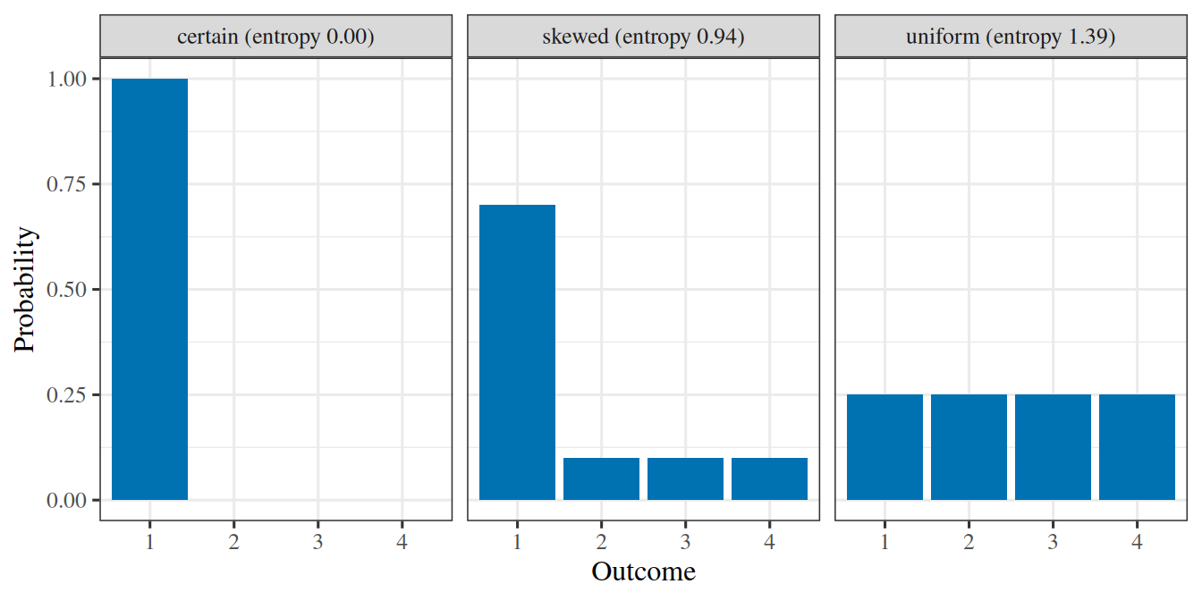
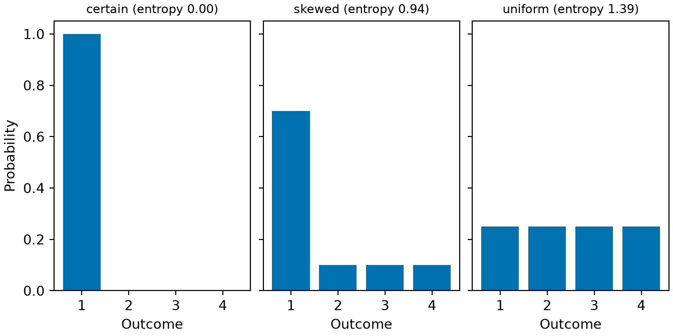
so \(H(\vp, \vp) \le \log M\), with equality exactly when \(\vp = \vu\). A certain outcome has zero entropy. The uniform distribution has the maximum entropy.

ExrExercise 47 (Three names for the same optimization (part 10))

Exercise 47 (Three names for the same optimization (part 10)) Use the setup of Exercise 38.

\(\lpnorm{2}\) regularization replaces \(\emprisk\) by \(\emprisk + \regpar\sumto{k}{\ninputvars}\coef{k}^2\), summing from \(k = 1\) so that the intercept \(\coef{0}\) is unpenalized. Determine how penalizing \(\coef{0}\) would alter the intercept score equation of Exercise 52, and use that result to explain why \(\coef{0}\) is left unpenalized.

SolutionSolution 47

Solution 47. Differentiate the objective \(\empriskf{\vcoef} + \regpar\sum_{k \ge 1}\coef{k}^2\) with respect to \(\coef{0}\). Unpenalized, the intercept column of \(\design(\mx)\) is ones, so

\[ \begin{aligned} \frac{\partial \emprisk}{\partial\coef{0}} &= -\frac1n\sum_i\paren{y_i - \prob_i} \\ &= 0 \end{aligned} \quad\Longrightarrow\quad \sum_i \prob_i = \sum_i y_i, \]

which is Exercise 52: the fitted probabilities sum to the observed number of positive outcomes.

Now add \(\regpar\coef{0}^2\) to the objective. The stationarity condition becomes \(-\tfrac1n\sum_i(y_i - \prob_i) + 2\regpar\coef{0} = 0\), that is

\[\sum_i \prob_i = \sum_i y_i - 2n\regpar\hcoef{0} .\]

Aggregate calibration no longer holds, and the difference between \(\sum_i \prob_i\) and \(\sum_i y_i\) does not depend on the predictors. Because the penalty shrinks \(\hcoef{0}\) toward \(0\), and \(\coef{0} = 0\) corresponds to a baseline probability of \(\tfrac12\), shrinking \(\coef{0}\) biases the average predicted probability toward \(\tfrac12\): rare outcomes are systematically over-predicted and common outcomes are systematically under-predicted.

A second reason is invariance to predictor location. A penalty on a slope \(\coef{k}\) penalizes large rates of change with respect to \(x_k\). The intercept is not a rate of change. Centering a predictor, \(x_k \mapsto x_k - \bar x_k\), changes \(\hcoef{0}\) and leaves every slope unchanged, so penalizing \(\coef{0}\) makes the fitted probabilities depend on the choice of origin for the predictors. Standardizing the predictors puts the slopes on a common scale, while the intercept still depends on the overall outcome prevalence.

LemTheorem 10 (Cross-entropy is smallest at the true distribution)

Theorem 10 (Cross-entropy is smallest at the true distribution) For distributions \(\vp\) and \(\vq\) over the same outcomes with \(q_j > 0\) wherever \(p_j > 0\),

\[ H(\vp, \vq) \ge H(\vp, \vp), \]

with equality only when \(\vq = \vp\). A term with \(p_j = 0\) contributes \(0\), by the convention \(0 \log 0 = 0\). If \(q_j = 0\) for some \(j\) with \(p_j > 0\), then \(H(\vp, \vq) = \infty\) and the inequality holds trivially. The difference is the Kullback–Leibler divergence \(D_{\mathrm{KL}}(\vp \,\|\, \vq) \ge 0\).

ProofProof

Proof. This is the solution to Exercise 43: see Solution 43.

ExmExample 20 (Cross-entropy against a wrong guess)

Example 20 (Cross-entropy against a wrong guess) Let \(\vp = (0.9, 0.1)\) be the true distribution and \(\vq = (0.5, 0.5)\) a guess.

ce_p <- c(0.9, 0.1)
ce_q <- c(0.5, 0.5)
ce_pq <- -sum(ce_p * log(ce_q))
ce_pp <- -sum(ce_p * log(ce_p))
c(H_pq = ce_pq, H_pp = ce_pp, KL = ce_pq - ce_pp)

     H_pq      H_pp        KL 
0.6931472 0.3250830 0.3680642 

Here \(H(\vp, \vq) = 0.693 \ge H(\vp, \vp) = 0.325\), as Theorem 10 says. The gap \(D_{\mathrm{KL}}(\vp \,\|\, \vq) = 0.368\) is positive because \(\vq \ne \vp\).

library(ggplot2)
ce_curve <- data.frame(q1 = seq(0.02, 0.98, length.out = 300))
ce_curve$ce <- -(ce_p[1] * log(ce_curve$q1) + ce_p[2] * log(1 - ce_curve$q1))
ggplot(ce_curve, aes(q1, ce)) +
  geom_line(colour = "#0072B2") +
  geom_vline(xintercept = ce_p[1], linetype = "dashed") +
  geom_point(
    data = data.frame(q1 = ce_q[1], ce = ce_pq),
    colour = "#D55E00", shape = 17, size = 3
  ) +
  labs(x = "Guessed probability of the first outcome", y = "Cross-entropy")

import matplotlib.pyplot as plt
import numpy as np

p_ce = np.array([0.9, 0.1])
q1_ce = np.linspace(0.02, 0.98, 300)
fig, ax = plt.subplots(figsize=(5, 4), layout="constrained")
ax.plot(q1_ce, -(p_ce[0] * np.log(q1_ce) + p_ce[1] * np.log(1 - q1_ce)), color="#0072B2");
ax.axvline(p_ce[0], color="black", linestyle="--");
ax.plot(0.5, -(p_ce[0] * np.log(0.5) + p_ce[1] * np.log(0.5)), color="#D55E00", marker="^", markersize=9, linestyle="");
ax.set_xlabel("Guessed probability of the first outcome");
ax.set_ylabel("Cross-entropy");
plt.show()

Figure 17: The cross-entropy \(H(\vp, \vq)\) of Example 20 as the guess \(\vq = (q_1, 1 - q_1)\) varies, when the truth is \(\vp = (0.9, 0.1)\). It is lowest where the guess equals the truth (dashed), and the guess \((0.5, 0.5)\) of the example (triangle) lies above that minimum.

R

(a)

Python

(b)

LemTheorem 11 (The range of the entropy)

Theorem 11 (The range of the entropy) A distribution \(\vp\) over \(M\) outcomes has

\[ 0 \le H(\vp, \vp) \le \log M. \]

The minimum \(0\) holds exactly when one outcome is certain, and the maximum \(\log M\) exactly when \(\vp\) is uniform.

ProofProof

Proof. This is the solution to Exercise 46: see Solution 46.

ExmExample 21 (Entropy of three distributions over four outcomes)

Example 21 (Entropy of three distributions over four outcomes)  

en_entropy <- function(p) -sum(ifelse(p > 0, p * log(p), 0))
en_dists <- list(
  certain = c(1, 0, 0, 0),
  skewed = c(0.7, 0.1, 0.1, 0.1),
  uniform = rep(0.25, 4)
)
vapply(en_dists, en_entropy, numeric(1))

 certain   skewed  uniform 
0.000000 0.940448 1.386294 

With \(M = 4\) outcomes, Theorem 11 puts the entropy between \(0\) and \(\log 4 = 1.386\). The certain distribution has entropy \(0\), the uniform distribution has entropy \(\log 4\), and the skewed distribution has entropy at 0.94, in-between the other two.

library(ggplot2)
enf <- do.call(rbind, lapply(names(en_dists), function(nm) {
  data.frame(
    distribution = sprintf("%s (entropy %.2f)", nm, en_entropy(en_dists[[nm]]) + 0),
    outcome = factor(1:4),
    prob = en_dists[[nm]]
  )
}))
enf$distribution <- factor(enf$distribution, levels = unique(enf$distribution))
ggplot(enf, aes(outcome, prob)) +
  geom_col(fill = "#0072B2") +
  facet_wrap(vars(distribution)) +
  labs(x = "Outcome", y = "Probability")

import matplotlib.pyplot as plt
import numpy as np

def entropy_enf(p):
    p = np.asarray(p, float)
    return -np.sum(np.where(p > 0, p * np.log(np.where(p > 0, p, 1)), 0))

dists_enf = {
    "certain": [1, 0, 0, 0],
    "skewed": [0.7, 0.1, 0.1, 0.1],
    "uniform": [0.25] * 4,
}
fig, axes = plt.subplots(1, 3, figsize=(7, 3.5), sharey=True, layout="constrained")
for ax, (name, p) in zip(axes, dists_enf.items()):
    ax.bar(range(1, 5), p, color="#0072B2");
    ax.set_title(f"{name} (entropy {entropy_enf(p) + 0.0:.2f})", fontsize=9);
    ax.set_xticks(range(1, 5));
    ax.set_xlabel("Outcome");
axes[0].set_ylabel("Probability");
plt.show()

Figure 18: The three distributions of Example 21 put their probability on four outcomes. The entropy rises from \(0\), when one outcome has all of the probability, to \(\log 4\), when the distribution spreads it evenly.

R

(a)

Python

(b)

5.1 Where cross-entropy comes from

Cross-entropy is not a machine learning invention. It comes from Claude Shannon’s 1948 theory of communication [16], where it measures the average number of bits per symbol required when encoding a source with a code designed for another distribution.

For a source that emits symbol \(j\) with probability \(p_j\), no uniquely decodable code averages fewer than \(H(\vp, \vp)\) bits per symbol, the base-\(2\) entropy of Theorem 11. A code built for a distribution \(\vq\) uses on average about the base-\(2\) cross-entropy \(H(\vp, \vq)\) bits per symbol. The difference \(D_{\mathrm{KL}}(\vp \,\|\, \vq)\) of Theorem 10 is the average number of extra bits per symbol required by using \(\vq\) instead of \(\vp\), and it is zero if and only if \(\vq = \vp\). For the source-coding theorems behind these bounds, see Source Coding in Information Theory for Data Science.

Minimizing cross-entropy over \(\vq\) brings \(\vq\) closer to \(\vp\), and fitting a logistic regression does this at each observation. The reference distribution \(\vp\) places probability \(1\) on the observed label and \(0\) on the other outcome, while the model’s distribution \(\vq\) is \((1 - \prob, \prob)\). A distribution that places probability \(1\) on a single outcome has entropy \(0\), so for a labeled training point the cross-entropy and the Kullback–Leibler divergence are equal.

The base of the logarithm chooses the unit of information. Base \(2\) measures information in bits, and the natural logarithm measures it in nats. Since \(\log_2 z = \ln z / \ln 2\), switching between them multiplies every term by a positive constant, so it does not change the minimizer. Throughout this chapter \(\log\) denotes the natural logarithm, so the losses are measured in nats.

VideosWatch

• Weinberger fits logistic regression by maximum likelihood, from 30:50 [10], Lecture 11.
• Starmer also fits logistic regression by maximum likelihood [17].
• He explains cross-entropy [18] as a loss for a neural network’s classifier.

ReadingRead

GeeksforGeeks explains binary cross-entropy [19].

6 The gradient

There is no closed-form expression for \(\hvcoef\), so we compute it iteratively by the methods of the gradient descent chapter. Those methods require the gradient of the log loss. Exercise 48 shows that the derivative of the logistic function cancels in this gradient, leaving an expression of the same form as in linear regression.

ExrExercise 48 (The gradient, and the factor that cancels)

Exercise 48 (The gradient, and the factor that cancels) Let \(z_i = \dprod{\vcoef}{\vx_i}\), \(\prob_i = \sigmoid(z_i)\), and \(C_i = -y_i\log \prob_i - (1-y_i)\log(1 - \prob_i)\) be observation \(i\)’s contribution to the log loss of Exercise 31.

Show that \(\dfrac{\partial C_i}{\partial z_i} = \prob_i - \outvar_i\). Use \(\sigmoid' = \sigmoid(1-\sigmoid)\) from Exercise 9, and do not split into cases.

SolutionSolution 48

Solution 48. Differentiate the two terms and substitute \(\sigmoid'(z_i) = \prob_i(1 - \prob_i)\):

\[ \begin{aligned} \frac{\partial C_i}{\partial z_i} &= -y_i\,\frac{\sigmoid'(z_i)}{\prob_i} + (1 - y_i)\,\frac{\sigmoid'(z_i)}{1 - \prob_i} \\ &= -y_i\,\frac{\prob_i(1-\prob_i)}{\prob_i} + (1 - y_i)\,\frac{\prob_i(1-\prob_i)}{1 - \prob_i} \end{aligned} \]

The \(\prob_i\) cancels in the first term and the \(1 - \prob_i\) in the second:

\[ \begin{aligned} &= -y_i\paren{1 - \prob_i} + \paren{1 - y_i}\prob_i \\ &= -y_i + y_i\prob_i + \prob_i - y_i\prob_i \\ &= \prob_i - y_i \end{aligned} \]

The derivative of the cost with respect to the score is the residual: predicted probability minus observed label. Nothing is left of the exponentials, and nothing is left of \(\sigmoid'\).

ExrExercise 49 (The gradient, and the factor that cancels (part 2))

Exercise 49 (The gradient, and the factor that cancels (part 2)) Use the setup of Exercise 48.

Hence give \(\grad_{\vcoef} C\) for the whole dataset, first as a sum over observations and then in matrix form, where \(\design(\mx)\) is the \(\nobs \times (\ninputvars+1)\) design matrix and \(\vprob\) is the vector of fitted probabilities.

SolutionSolution 49

Solution 49. \(z_i = \dprod{\vcoef}{\vx_i}\), so \(\grad_{\vcoef} z_i = \vx_i\), and the chain rule gives

\[ \begin{aligned} \grad_{\vcoef} C &= \suminf{\prob_i - y_i}\vx_i \\ &= X^\top\paren{\vprob - \vy} \end{aligned} \]

Least squares has gradient \(\design(\mx)^\top(\design(\mx)\vcoef - \vy)\), which is the same expression with \(\vprob\) in place of the linear fit \(\design(\mx)\vcoef\). The two models have identical gradient structure: design matrix transposed, times residual. Only the link from \(\vcoef\) to the fitted value differs, and that difference is exactly what stops the equation having a closed-form solution — see why we cannot just solve for it.

One observation at a time, the residual shows what each point does to a descent step \(\vcoef \leftarrow \vcoef - \learnrate\,\grad_{\vcoef} C\):

• If \(y_i = 0\) and \(\prob_i \approx 0\), or \(y_i = 1\) and \(\prob_i \approx 1\), the residual is near zero, and the point barely changes the gradient.
• If \(y_i = 1\) and \(\prob_i \approx 0\), the step adds in about \(\learnrate\,\vx_i\) — a larger inner product gives a larger prediction.
• If \(y_i = 0\) and \(\prob_i \approx 1\), the step subtracts about \(\learnrate\,\vx_i\) — a smaller inner product gives a smaller prediction.

The magnitude of the residual, \(\abs{\prob_i - \outvar_i}\), is the probability that the model assigns to the opposite label \(1 - \outvar_i\). Each observation therefore contributes to the gradient in the direction of its feature vector \(\vx_i\), weighted by the model’s predicted probability of misclassifying that observation.

ExrExercise 50 (The gradient, and the factor that cancels (part 3))

Exercise 50 (The gradient, and the factor that cancels (part 3)) Use the setup of Exercise 48.

Exercise 48 has a factor that cancels. Differentiate the squared-error cost \(S_i = \tfrac{1}{2}\paren{\prob_i - \outvar_i}^2\) with respect to \(z_i\) instead, and compare the two derivatives at \(z_i = 8\) with \(\outvar_i = 0\), an observation for which the predicted probability is close to \(1\) while the observed label is \(0\). Report the ratio.

SolutionSolution 50

Solution 50. By the chain rule,

\[ \begin{aligned} \frac{\partial S_i}{\partial z_i} &= \paren{\prob_i - y_i}\sigmoid'(z_i) \\ &= \paren{\prob_i - y_i}\prob_i\paren{1 - \prob_i} \end{aligned} \]

The factor \(\sigmoid'(z_i)\) remains in the derivative because squared error has no logarithm to cancel it.

At \(z_i = 8\) with \(y_i = 0\):

\[ \begin{aligned} \prob_i &= \sigmoid(8) \\ &= 0.99966, \end{aligned} \]

so

• log loss: \(\prob_i - \outvar_i = 0.99966\)
• squared error: \(0.99966 \times 0.99966 \times 0.00033535 = 3.351 \times 10^{-4}\)

The log-loss derivative is about \(2983\) times larger than the squared-error derivative.

Although the model assigns probability \(0.9997\) to the wrong class, squared error produces a gradient of only \(3.35 \times 10^{-4}\), so gradient descent makes negligible progress. This vanishing-gradient behavior makes squared error unsuitable for saturating outputs, whereas in Solution 48 the factor \(1/\prob_i\) from differentiating the logarithm cancels \(\sigmoid'(z_i)\).

Exercise 10 showed that \(\sigmoid\) is nearly flat far from the decision boundary. Log loss is constructed so that this flatness does not diminish the gradient on misclassified observations.

ExrExercise 51 (The gradient, and the factor that cancels (part 4))

Exercise 51 (The gradient, and the factor that cancels (part 4)) Use the setup of Exercise 48.

Show that \(\norm{\grad_{\vcoef} C_i} < \norm{\vx_i}\) for every \(\vcoef\), and say what that guarantees.

SolutionSolution 51

Solution 51. Because \(\grad_{\vcoef} C_i = (\prob_i - y_i)\vx_i\), we have \(\norm{\grad_{\vcoef} C_i} = \abs{\prob_i - y_i} \cdot \norm{\vx_i}\). Since \(\prob_i \in (0,1)\) by Exercise 7 and \(\outvar_i \in \{0,1\}\), \(\abs{\prob_i - \outvar_i} < 1\) and the bound follows.

This bound guarantees that no single observation can produce a gradient larger in norm than \(\norm{\vx_i}\), regardless of how large the classification error is. The contribution of any single observation to a gradient step is bounded by the norm of its feature vector, which is one reason to standardize features on different scales before fitting.

Applying the same bound to the second derivative yields an explicit step-size condition. The Hessian is \(\design(\mx)^\top W \design(\mx)\) with \(W = \diagf{\prob_i(1-\prob_i)}\), and Exercise 10 showed that every \(\prob_i(1-\prob_i) \le 1/4\). Every eigenvalue of the Hessian is therefore at most \(\tfrac{1}{4}\eigval_{\max}\paren{X^\top X}\) for all \(\vcoef\).

This uniform curvature bound determines a safe step size. The step-size bound shows the stability condition \(\learnrate < 2/\eigval_{\max}\paren{\grad^2 C}\) for a quadratic objective. Using the uniform upper bound \(\tfrac{1}{4}\eigval_{\max}\paren{X^\top X}\) on the eigenvalues of \(\grad^2 C\) gives

\[\learnrate < \frac{8}{\eigval_{\max}\paren{X^\top X}}\]

Exercise 64 evaluates this bound on a small dataset where it gives \(\learnrate < 4/3\), compared with the exact local stability threshold of \(3/2\). In practice, a line search chooses step sizes adaptively without computing \(\eigval_{\max}\paren{X^\top X}\).

ExrExercise 52 (The gradient, and the factor that cancels (part 5))

Exercise 52 (The gradient, and the factor that cancels (part 5)) Use the setup of Exercise 48.

At the maximum the gradient vanishes, giving the score equations \(\design(\mx)^\top(\vprob - \vy) = \vzero\). Suppose the first column of \(\design(\mx)\) is a column of ones, and the second is a binary indicator \(\predvar_{i} \in \{0, 1\}\) for membership of some group. State in words what each of those two equations says about the fitted model.

SolutionSolution 52

Solution 52. The column of ones gives \(\sum_i \prob_i = \sum_i \outvar_i\): the sum of the fitted probabilities equals the observed number of positive outcomes. A logistic regression with an intercept is therefore calibrated in aggregate on the training set: if \(30\) of \(100\) training observations have \(y_i = 1\), the fitted probabilities sum to \(30\).

The binary indicator gives \(\sum_{i \,:\, x_i = 1} \prob_i = \sum_{i \,:\, x_i = 1} y_i\), so the same equality holds within the subgroup where \(x_i = 1\). Subtracting this subgroup equation from the intercept equation shows that it also holds in the complementary subgroup where \(x_i = 0\).

Each indicator feature therefore enforces aggregate calibration within the subgroup it defines, and a categorical predictor encoded with indicator variables forces the fitted probabilities to match the observed positive counts in every level of the predictor. The model cannot be miscalibrated in aggregate on any subgroup represented in the design matrix, though it can be miscalibrated on subgroups defined by variables omitted from the model, which motivates checking calibration across held-out subgroup definitions.

DefDefinition 4 (Residual of a logistic regression)

Definition 4 (Residual of a logistic regression) The residual of observation \(i\) in logistic regression is its predicted probability minus its label,

\[ \prob_i - \outvar_i, \qquad \prob_i = \sigmoidf{\dprod{\vcoef}{\vpredvar_i}}. \]

It is the negative of the response residual \(\outvar_i - \prob_i\), and it is in \((-1, 1)\).

ExmExample 22 (Residuals of two men in the WCGS data)

Example 22 (Residuals of two men in the WCGS data) The first man in data/wcgs.csv with coronary heart disease has \(\outvar_i = 1\) and fitted probability \(\prob_i = 0.069\), so his residual is \(\prob_i - \outvar_i = -0.931\). The first man without it has \(\outvar_i = 0\) and \(\prob_i = 0.134\), so his residual is \(0.134\).

library(ggplot2)
lrv_pts <- data.frame(
  label = c(1, 0),
  prob = 0.9,
  kind = factor(c("label 1", "label 0"), levels = c("label 1", "label 0"))
)
ggplot(lrv_pts, aes(x = label, y = label, colour = kind)) +
  geom_hline(yintercept = 0.9, linetype = "dashed", colour = "grey50") +
  geom_segment(aes(xend = label, y = label, yend = prob, linetype = kind), linewidth = 1) +
  geom_point(aes(shape = kind), size = 3) +
  scale_x_continuous(breaks = c(0, 1)) +
  scale_colour_manual(values = c("label 1" = "#0072B2", "label 0" = "#D55E00")) +
  scale_shape_manual(values = c("label 1" = 16, "label 0" = 17)) +
  scale_linetype_manual(values = c("label 1" = "solid", "label 0" = "dashed")) +
  labs(
    x = "Label", y = "Label and predicted probability (dashed line)",
    colour = NULL, shape = NULL, linetype = NULL
  )

import matplotlib.pyplot as plt

fig, ax = plt.subplots(figsize=(6, 4), layout="constrained")
ax.axhline(0.9, color="grey", linestyle="--");
ax.vlines(1, 0.9, 1, color="#0072B2", linestyle="-", linewidth=2);
ax.plot(1, 1, color="#0072B2", marker="o", markersize=8, linestyle="", label="label 1");
ax.vlines(0, 0, 0.9, color="#D55E00", linestyle="--", linewidth=2);
ax.plot(0, 0, color="#D55E00", marker="^", markersize=8, linestyle="", label="label 0");
ax.set_xticks([0, 1]);
ax.set_xlabel("Label");
ax.set_ylabel("Label and predicted probability (dashed line)");
fig.legend(loc="outside lower center", ncol=2);
plt.show()

Figure 19: The two points of Example 22, which share the probability \(0.9\) that the model gives to a label of \(1\). The vertical distance from the dashed line to each point is the size of its residual: small for the label \(1\), large for the label \(0\).

R

(a)

Python

(b)

LemTheorem 12 (Derivative of the log loss with respect to the score)

Theorem 12 (Derivative of the log loss with respect to the score) Let \(z_i = \dprod{\vcoef}{\vpredvar_i}\) and \(\prob_i = \sigmoidf{z_i}\). Observation \(i\)’s contribution to the log loss of Definition 3 has derivative

\[ \derivf{C_i}{z_i} = \prob_i - \outvar_i, \]

the residual of Definition 4.

ProofProof

Proof. By Solution 48.

ExmExample 23 (The residual of a man with a body mass index of 25)

Example 23 (The residual of a man with a body mass index of 25) A man with \(\text{bmi} = 25\) has \(\prob_i = 0.083\) in the model of Example 2 (Example 3). If he has coronary heart disease, \(\outvar_i = 1\) and \(\derivf{C_i}{z_i} = \prob_i - 1 = -0.917\). If he does not, \(\outvar_i = 0\) and the derivative is \(\prob_i = 0.083\): the derivative is about \(11\) times as large in magnitude when the label is \(1\), because the model had judged his disease unlikely.

library(ggplot2)
lrf_bars <- data.frame(
  label = factor(c("label 1", "label 0"), levels = c("label 1", "label 0")),
  derivative = c(plogis(2) - 1, plogis(2) - 0)
)
ggplot(lrf_bars, aes(label, derivative, fill = label, linetype = label)) +
  geom_hline(yintercept = 0, colour = "grey40") +
  geom_col(colour = "black", width = 0.6) +
  scale_fill_manual(values = c("label 1" = "#0072B2", "label 0" = "#D55E00")) +
  scale_linetype_manual(values = c("label 1" = "solid", "label 0" = "dashed")) +
  labs(x = NULL, y = "Derivative of the loss", fill = NULL, linetype = NULL)

import matplotlib.pyplot as plt
from scipy.special import expit

fig, ax = plt.subplots(figsize=(6, 4), layout="constrained")
ax.axhline(0, color="grey");
ax.bar(["label 1"], [expit(2) - 1], color="#0072B2", edgecolor="black", width=0.6);
ax.bar(["label 0"], [expit(2) - 0], color="#D55E00", edgecolor="black", linestyle="--", width=0.6);
ax.set_ylabel("Derivative of the loss");
plt.show()

Figure 20: The derivative of the loss for the two points of Example 23, which have the same score. The point with the label \(0\) is much farther from the probability the model gives it, so its derivative is much larger.

R

(a)

Python

(b)

LemTheorem 13 (Gradient of the log loss)

Theorem 13 (Gradient of the log loss) The gradient of the log loss of Definition 3 with respect to \(\vcoef\) is

\[ \grad C(\vcoef) = \sumin \paren{\prob_i - \outvar_i} \vpredvar_i = \tp{\design} \paren{\vprob - \voutvar}, \]

where \(\design\) is the design matrix, with the constant column of ones that absorbs the intercept, and \(\vprob\) is the vector of fitted probabilities.

ProofProof

Proof. By Theorem 12 and the chain rule, as in Solution 49.

ExmExample 24 (The gradient at zero coefficients)

Example 24 (The gradient at zero coefficients) Consider six points with predictor values \(1, \dots, 6\) and labels \(0, 0, 1, 0, 1, 1\), evaluated at \(\vcoef = \vzero\). Every fitted probability is then \(\prob_i = \sigmoidf{0} = 1/2\). The intercept entry of \(\tp{\design} \paren{\vprob - \voutvar}\) is \(\sumin \paren{1/2 - \outvar_i} = 0\). The slope entry is \(\sumin \paren{1/2 - \outvar_i} \predvar_i = -3.5\). The negative slope entry says that the loss falls as the slope increases, so a first step of gradient descent raises the slope.

library(ggplot2)
lgg_pts <- data.frame(
  x = 1:6,
  label = factor(c(0, 0, 1, 0, 1, 1), levels = c(1, 0))
)
ggplot(lgg_pts, aes(x, as.numeric(as.character(label)), colour = label)) +
  geom_hline(yintercept = 0.5, linetype = "dashed", colour = "grey50") +
  geom_segment(
    aes(xend = x, yend = 0.5, linetype = label), linewidth = 1
  ) +
  geom_point(aes(shape = label), size = 3) +
  scale_colour_manual(values = c("1" = "#0072B2", "0" = "#D55E00")) +
  scale_shape_manual(values = c("1" = 16, "0" = 17)) +
  scale_linetype_manual(values = c("1" = "solid", "0" = "dashed")) +
  scale_x_continuous(breaks = 1:6) +
  labs(x = "Predictor", y = "Label", colour = "Label", shape = "Label", linetype = "Label")

import matplotlib.pyplot as plt
import numpy as np

x_lgg = np.arange(1, 7)
y_lgg = np.array([0, 0, 1, 0, 1, 1])
fig, ax = plt.subplots(figsize=(6, 4), layout="constrained")
ax.axhline(0.5, color="grey", linestyle="--");
for label_lgg, colour, marker, style in [(1, "#0072B2", "o", "-"), (0, "#D55E00", "^", "--")]:
    keep_lgg = y_lgg == label_lgg
    ax.vlines(x_lgg[keep_lgg], 0.5, y_lgg[keep_lgg], color=colour, linestyle=style, linewidth=2);
    ax.plot(x_lgg[keep_lgg], y_lgg[keep_lgg], color=colour, marker=marker, markersize=8,
            linestyle="", label=f"label {label_lgg}");
ax.set_xticks(x_lgg);
ax.set_xlabel("Predictor");
ax.set_ylabel("Label");
fig.legend(loc="outside lower center", ncol=2);
plt.show()

Figure 21: The six points of Example 24, with the fitted probability \(1/2\) that they all have at zero coefficients (dashed line). Each vertical segment is the distance between a point’s label and that probability, which is the size of its residual.

R

(a)

Python

(b)

LemTheorem 14 (Hessian of the log loss)

Theorem 14 (Hessian of the log loss) The Hessian of the log loss of Definition 3 with respect to \(\vcoef\) is

\[ \begin{aligned} \grad^2 C(\vcoef) &= \sumin \prob_i \paren{1 - \prob_i} \vpredvar_i \tp{\vpredvar_i} \\ &= \tp{\design} W \design, \end{aligned} \]

where \(W\) is the diagonal matrix with entries \(\prob_i \paren{1 - \prob_i}\). Because each \(\prob_i \paren{1 - \prob_i} > 0\), \(\tp{\design} W \design\) is positive semidefinite for every \(\vcoef\), so \(C(\vcoef)\) is convex and therefore a friendly loss.

ProofProof

Proof. By Theorem 13, \(\grad C(\vcoef) = \sumin \paren{\prob_i - \outvar_i} \vpredvar_i\). Only \(\prob_i\) depends on \(\vcoef\), and by Theorem 2 and the chain rule its gradient is \(\prob_i \paren{1 - \prob_i} \vpredvar_i\). Differentiating each term of the sum gives \(\prob_i \paren{1 - \prob_i} \vpredvar_i \tp{\vpredvar_i}\), and the sum of these is \(\tp{\design} W \design\).

ExmExample 25 (The Hessian at zero coefficients)

Example 25 (The Hessian at zero coefficients) For the six points of Example 24 at \(\vcoef = \vzero\), every \(\prob_i = 1/2\), so \(W = \tfrac14 I\).

# the six points, with the column of ones for the intercept
x <- 1:6
design <- cbind(1, x)
# fitted probabilities at zero coefficients, and their weights p (1 - p)
p <- rep(1 / 2, 6)
w <- p * (1 - p)
# the Hessian: design' W design
crossprod(design, w * design)

           x
  1.50  5.25
x 5.25 22.75

The intercept entry is \(\tfrac14 \cdot 6 = 1.5\), the off-diagonal entry is \(\tfrac14 \sum_i \predvar_i = 5.25\), and the slope entry is \(\tfrac14 \sum_i \predvar_i^2 = 22.75\).

library(ggplot2)
hsf_x <- 1:6
hsf_design <- cbind(1, hsf_x)
hsf_h <- crossprod(hsf_design, (1 / 4) * hsf_design)
hsf_cells <- expand.grid(row = c("intercept", "slope"), col = c("intercept", "slope"))
hsf_cells$value <- as.vector(hsf_h)
ggplot(hsf_cells, aes(col, row, fill = value)) +
  geom_tile(colour = "white") +
  geom_text(aes(label = value), colour = "black", size = 5) +
  scale_fill_gradient(low = "#F0E442", high = "#56B4E9") +
  scale_y_discrete(limits = c("slope", "intercept")) +
  labs(x = "Column", y = "Row", fill = "Entry")

import matplotlib.pyplot as plt
from matplotlib.colors import LinearSegmentedColormap
import numpy as np

x_hsf = np.arange(1, 7)
design_hsf = np.column_stack([np.ones(6), x_hsf])
h_hsf = design_hsf.T @ (0.25 * design_hsf)
fig, ax = plt.subplots(figsize=(6, 4), layout="constrained")
im = ax.imshow(h_hsf, cmap=LinearSegmentedColormap.from_list("hsf", ["#F0E442", "#56B4E9"]))
for i in range(2):
    for j in range(2):
        ax.text(j, i, f"{h_hsf[i, j]:g}", ha="center", va="center", fontsize=14);
ax.set_xticks([0, 1], ["intercept", "slope"]);
ax.set_yticks([0, 1], ["intercept", "slope"]);
ax.set_xlabel("Column");
ax.set_ylabel("Row");
fig.colorbar(im, ax=ax, label="Entry");
plt.show()

Figure 22: The Hessian of Example 25 at zero coefficients. The slope entry is far larger than the intercept entry because it sums the squared values of the feature.

R

(a)

Python

(b)

LemTheorem 15 (The residuals are orthogonal to every predictor at a minimizer)

Theorem 15 (The residuals are orthogonal to every predictor at a minimizer) At any finite minimizer \(\hat{\vcoef}\) of the log loss, the gradient vanishes:

\[ \tp{\design} \paren{\vprob - \voutvar} = \vzero. \]

Each column of \(\design\) is orthogonal to the residuals, and the column of ones makes the residuals sum to zero.

ProofProof

Proof. The log loss is differentiable and \(\hat{\vcoef}\) minimizes it over all coefficient vectors, so its gradient is zero there. By Theorem 13, that gradient is \(\tp{\design} \paren{\vprob - \voutvar}\). The \(j\)th entry of this vector is the dot product of the \(j\)th column of \(\design\) with the residuals, and the entry for the column of ones is \(\sumin \paren{\prob_i - \outvar_i}\).

ExmExample 26 (Residuals at the fitted coefficients)

Example 26 (Residuals at the fitted coefficients) Fit a logistic regression with an intercept to the six points of Example 24, and compute \(\tp{\design} \paren{\vprob - \voutvar}\).

# the six points
x <- 1:6
y <- c(0, 0, 1, 0, 1, 1)
# the fit, and its design matrix with the column of ones
fit <- glm(y ~ x, family = binomial)
design <- model.matrix(fit)
# the residuals: fitted probabilities minus labels
residual <- fitted(fit) - y
# the gradient, rounded to six decimals
round(drop(crossprod(design, residual)), 6)

(Intercept)           x 
          0           0 

Both entries are zero to six decimals, as Theorem 15 requires.

library(ggplot2)
lst_pts <- data.frame(
  x = x,
  label = factor(y, levels = c(1, 0)),
  y = y,
  fitted = fitted(fit)
)
lst_curve <- data.frame(x = seq(1, 6, length.out = 100))
lst_curve$prob <- predict(fit, newdata = lst_curve, type = "response")
ggplot(lst_pts, aes(x, y, colour = label)) +
  geom_line(data = lst_curve, aes(y = prob), colour = "grey50") +
  geom_segment(aes(xend = x, yend = fitted, linetype = label), linewidth = 1) +
  geom_point(aes(shape = label), size = 3) +
  scale_colour_manual(values = c("1" = "#0072B2", "0" = "#D55E00")) +
  scale_shape_manual(values = c("1" = 16, "0" = 17)) +
  scale_linetype_manual(values = c("1" = "solid", "0" = "dashed")) +
  scale_x_continuous(breaks = 1:6) +
  labs(x = "Predictor", y = "Label and fitted probability", colour = "Label", shape = "Label",
       linetype = "Label")

import matplotlib.pyplot as plt

points_lst = r.lst_pts
curve_lst = r.lst_curve
fig, ax = plt.subplots(figsize=(6, 4), layout="constrained")
ax.plot(curve_lst["x"], curve_lst["prob"], color="grey");
for label_lst, colour, marker, style in [(1, "#0072B2", "o", "-"), (0, "#D55E00", "^", "--")]:
    keep_lst = points_lst["y"] == label_lst
    sub_lst = points_lst[keep_lst]
    ax.vlines(sub_lst["x"], sub_lst["fitted"], sub_lst["y"], color=colour, linestyle=style,
              linewidth=2);
    ax.plot(sub_lst["x"], sub_lst["y"], color=colour, marker=marker, markersize=8,
            linestyle="", label=f"label {label_lst}");
ax.set_xticks(range(1, 7));
ax.set_xlabel("Predictor");
ax.set_ylabel("Label and fitted probability");
fig.legend(loc="outside lower center", ncol=2);
plt.show()

Figure 23: The six points of Example 26 and their fitted probability (curve). Each vertical segment is the residual of one point. The solid segments and the dashed segments have the same total length, which is what a gradient of zero says about the intercept.

R

(a)

Python

(b)

ExrExercise 53 (Fitting by gradient descent, in code)

Exercise 53 (Fitting by gradient descent, in code) Simulate \(n = 400\) observations with two standard normal features \(x_1, x_2\) and labels drawn from \(\Pr[Y = 1 \mid \vx] = \sigmoid(-0.5 + 2x_1 - 1.5x_2)\), so the coefficients that produced the data are known to be \(\vcoef = (-0.5, 2, -1.5)\).

In Python, R or Julia, minimize the mean log loss \(J(\vcoef) = \tfrac1\nobs\sum_i C_i\) by gradient descent from \(\vcoef = \vzero\), with step size \(\learnrate = 0.5\) for \(10{,}000\) steps, using the gradient of Exercise 49. Say how that gradient’s sign and scale relate to the \(\tp{\design(\mx)}(\vy - \vprob)\) of Exercise 31’s log-likelihood.

SolutionSolution 53

Solution 53. The gradient of \(J\) is \(\tp{X}(\vprob - \vy)/n\), which is the log-likelihood’s \(\tp{X}(\vy - \vprob)\) with its sign flipped, because we are descending the negative log-likelihood rather than ascending the log-likelihood, and divided by \(n\). Dividing by \(\nobs\) changes no minimizer, as Exercise 38 showed, and makes a sensible step size independent of how much data there is.

Python

import numpy as np

sigmoid = lambda z: 0.5 * (1 + np.tanh(0.5 * z))

rng = np.random.default_rng(0)
n = 400
x1, x2 = rng.normal(size=n), rng.normal(size=n)
X = np.column_stack([np.ones(n), x1, x2])
y = (rng.random(n) < sigmoid(-0.5 + 2 * x1 - 1.5 * x2)).astype(float)

def J(b):
    p = sigmoid(X @ b)
    return -np.mean(y * np.log(p) + (1 - y) * np.log(1 - p))

def grad_J(b):
    return X.T @ (sigmoid(X @ b) - y) / n

beta = np.zeros(3)
for _ in range(10_000):
    beta = beta - 0.5 * grad_J(beta)

print(beta.round(2))          # true values: [-0.5, 2, -1.5]

[-0.54  1.95 -1.18]

print(J(beta).round(4))

0.4294

R

sigmoid <- function(z) 0.5 * (1 + tanh(0.5 * z))

set.seed(0)
n <- 400
x1 <- rnorm(n)
x2 <- rnorm(n)
X <- cbind(1, x1, x2) # nolint: object_name_linter. X matches the prose.
y <- as.numeric(runif(n) < sigmoid(-0.5 + 2 * x1 - 1.5 * x2))

J <- function(b) { # nolint: object_name_linter.
  p <- sigmoid(drop(X %*% b))
  -mean(y * log(p) + (1 - y) * log(1 - p))
}

grad_J <- function(b) drop(t(X) %*% (sigmoid(drop(X %*% b)) - y) / n) # nolint

beta <- c(0, 0, 0)
for (step in seq_len(10000)) beta <- beta - 0.5 * grad_J(beta)

round(beta, 2)                # true values: c(-0.5, 2, -1.5)

         x1    x2 
-0.53  1.98 -1.46 

round(J(beta), 4)

[1] 0.4201

Julia

using Random, LinearAlgebra, Statistics

sigmoid(z) = 0.5 .* (1 .+ tanh.(0.5 .* z));

Random.seed!(0);
n = 400;
x1, x2 = randn(n), randn(n);
X = [ones(n) x1 x2];
y = Float64.(rand(n) .< sigmoid(-0.5 .+ 2 .* x1 .- 1.5 .* x2));

function J(b)
    p = sigmoid(X * b)
    -mean(y .* log.(p) .+ (1 .- y) .* log.(1 .- p))
end;

grad_J(b) = X' * (sigmoid(X * b) .- y) ./ n;

beta = zeros(3);
for _ in 1:10_000
    global beta = beta - 0.5 .* grad_J(beta)
end

println(round.(beta, digits = 2))   # true values: [-0.5, 2, -1.5]

[-0.48, 1.97, -1.62]

println(round(J(beta), digits = 4))

0.4069

# @sol-fit-by-gradient-descent-part2: the Python estimate, its standard error, and the R estimate
py_beta <- py$beta
py_grad <- max(abs(py$grad_J(py_beta)))
py_fit <- glm(py$y ~ py$X[, 2] + py$X[, 3], family = binomial)
py_se <- summary(py_fit)$coefficients[3, "Std. Error"]
py_z <- abs(py_beta[3] - (-1.5)) / py_se
r_beta <- beta

# @sol-fit-by-gradient-descent-part3: the two sigmoid forms in double precision
sig_tanh <- function(z) 0.5 * (1 + tanh(0.5 * z))
sig_exp <- function(z) 1 / (1 + exp(-z))
far <- seq(-60, 0, by = 0.01)
tanh_far <- sig_tanh(far)
tanh_floor <- min(tanh_far[tanh_far > 0])
tanh_zero_from <- max(far[tanh_far == 0])
exp_at_700 <- sig_exp(-700)
near <- seq(-10, 10, by = 0.001)
abs_gap <- max(abs(sig_tanh(near) - sig_exp(near)))
rel_gap <- abs(sig_tanh(near) - sig_exp(near)) / sig_exp(near)
worst_z <- near[which.max(rel_gap)]
worst_p <- sig_exp(worst_z)
worst_ulps <- abs(sig_tanh(worst_z) - worst_p) / 2^(floor(log2(worst_p)) - 52)
fmt <- function(v, d = 2) formatC(v, format = "e", digits = d)

ExrExercise 54 (Fitting by gradient descent, in code (part 2))

Exercise 54 (Fitting by gradient descent, in code (part 2)) Use the setup of Exercise 53.

Compare the fitted coefficients with \((-0.5, 2, -1.5)\). If one of them differs from the true value by more than you expected, determine whether the optimizer terminated before converging or whether the difference comes from another source, and explain how to check.

SolutionSolution 54

Solution 54. The Python version recovers \((-0.54, 1.95, -1.18)\) against the \((-0.5, 2, -1.5)\) from which the data were generated. The iteration has converged: the largest entry of the gradient at the final iterate is 2.22e-16. That value -1.18 is the maximum likelihood estimate for this sample of \(400\) points.

The discrepancy from \(-1.5\) is sampling error: the standard error on that coefficient is 0.164, so -1.18 is 1.96 standard errors from \(-1.5\). The R tab illustrates this with an independent sample: it draws \(400\) observations from R’s random number generator and estimates -1.46 for the same coefficient. The difference in the Python estimate comes from the random sample rather than the optimizer.

ExrExercise 55 (Fitting by gradient descent, in code (part 3))

Exercise 55 (Fitting by gradient descent, in code (part 3)) Use the setup of Exercise 53.

Express the sigmoid as \(\tfrac12\paren{1 + \tanh(\logodds/2)}\) rather than \(1/(1 + \e{-\logodds})\). Exercise 11 shows that these are the same mathematical function. State whether they are the same floating-point computation.

SolutionSolution 55

Solution 55. They are not the same floating-point computation.

ExrExercise 56 (Fitting by gradient descent, in code (part 4))

Exercise 56 (Fitting by gradient descent, in code (part 4)) Use the setup of Exercise 53.

Compare their numerical behavior for large negative \(\logodds\).

SolutionSolution 56

Solution 56. The tanh form loses relative accuracy for negative \(\logodds\) much earlier than the exponential form.

The exponential form evaluates \(e^{-\logodds}\), which overflows to \(+\infty\) below about \(\logodds = -709\); dividing \(1\) by \(+\infty\) still returns \(0\). The tanh form never overflows, but loses relative accuracy for negative \(\logodds\). Adding \(1\) to \(\tanh(\logodds/2)\) rounds onto the floating-point grid near \(1\), so the smallest positive value it can return is 5.55e-17, and for \(\logodds \le -38.13\) it returns \(0\). By contrast, the exponential form evaluates to 9.9e-305 at \(\logodds = -700\).

In a loss function that evaluates \(\log(p)\), rounding \(p\) to \(0\) turns \(-700\) into \(-\infty\). That underflow does not occur in this simulation, where \(|\logodds|\) remains below \(10\), though the two forms still differ in relative error. In absolute terms the two forms differ by at most 2.22e-16 over \(|\logodds| \le 10\). In relative terms, which govern the accuracy of \(\log(p)\), the difference grows as \(p\) approaches \(0\): the maximum relative difference over \(|\logodds| \le 10\) is 5.81e-13, at \(\logodds = -9.987\), where \(p\) is 4.60e-05 and the two floating-point values differ by 3941 units in the last place (ulps). This loss of significant digits comes from catastrophic cancellation when adding \(1\) to \(\tanh(\logodds/2) \approx -1\), though it leaves more than enough digits over \(|\logodds| \le 10\). For extreme negative scores, neither intermediate probability should be formed: evaluating the log-likelihood directly from \(\logodds\) (for example, via \(\logodds - \log(1 + e^\logodds)\) for \(\logodds < 0\)) avoids forming \(p\) altogether.

ExrExercise 57 (Fitting by gradient descent, in code (part 5))

Exercise 57 (Fitting by gradient descent, in code (part 5)) Use the setup of Exercise 53.

Name the library call you would use instead in each language, and check whether it fits the same objective by default.

SolutionSolution 57

Solution 57. In practice you would call a library: glm(y ~ x1 + x2, family = binomial) in R, or LogisticRegression from scikit-learn in Python. Beware the Python one: scikit-learn applies an \(\lpnorm{2}\) penalty by default, so it fits the regularized problem of Exercise 47 and will not reproduce these numbers until you turn the penalty off.

7 A fit small enough to do by hand

For a balanced dataset of six patients in two groups, the maximum likelihood estimate has a closed-form solution. Solving this six-patient problem in full provides an exact benchmark for testing step sizes, Newton’s method, and standard errors in the exercises that follow.

ExrExercise 58 (A logistic regression you can fit by hand)

Exercise 58 (A logistic regression you can fit by hand) We randomize six patients to control or treatment, and record whether each recovers. Code the group as \(x_i = -1\) for control and \(x_i = +1\) for treatment, and let \(y_i = 1\) mean recovery.

group	\(x\)	\(n\)	recovered
control	\(-1\)	\(3\)	\(1\)
treatment	\(+1\)	\(3\)	\(2\)

Fit \(\Pr[Y = 1 \mid x] = \sigmoid(\coef{0} + \coef{1} x)\).

Give the design matrix \(\design(\mx)\), and evaluate \(\grad_{\vcoef}\,\ell = \design(\mx)^\top(\vy - \vprob)\) at \(\vcoef = \vzero\). Interpret each of its two components.

SolutionSolution 58

Solution 58. Order the patients control-first, and take the three control outcomes to be \(y = 0, 0, 1\) and the three treatment outcomes \(y = 0, 1, 1\):

\[X = \begin{bmatrix} 1 & -1 \\ 1 & -1 \\ 1 & -1 \\ 1 & 1 \\ 1 & 1 \\ 1 & 1 \end{bmatrix}, \qquad \vy = \begin{bmatrix} 0 \\ 0 \\ 1 \\ 0 \\ 1 \\ 1\end{bmatrix}\]

At \(\vcoef = \vzero\) every \(\prob_i = \sigmoid(0) = 1/2\), so \(\vy - \vprob = \pt{-\tfrac12, -\tfrac12, \tfrac12, -\tfrac12, \tfrac12, \tfrac12}\) and

\[\tp{X}\paren{\vy - \vprob} = \begin{bmatrix} 0 \\ 1 \end{bmatrix}\]

The intercept component is \(\sum_i (y_i - \prob_i) = 3 - 6 \times \tfrac12 = 0\). Three of six patients recovered, and the model at \(\vcoef = \vzero\) already predicts three, so there is nothing to correct: the starting point happens to be calibrated in aggregate, in the sense of Exercise 52.

The slope component is \(\sum_i x_i(y_i - \prob_i) = 1\), and it is positive. That says the residual is correlated with the feature: the group coded \(+1\) has more recoveries than the current model predicts and the group coded \(-1\) has fewer, so increasing \(\coef{1}\) will improve the fit. The gradient already shows the treatment effect before anything has been fitted.

ExrExercise 59 (A logistic regression you can fit by hand (part 2))

Exercise 59 (A logistic regression you can fit by hand (part 2)) Use the setup of Exercise 58.

Give the log loss at \(\vcoef = \vzero\), exactly and to four significant figures. Why is this the value for any dataset of six observations at \(\vcoef = \vzero\)?

SolutionSolution 59

Solution 59. Every \(\prob_i = 1/2\), so every observation contributes \(-\log \tfrac12 = \log 2\) whatever its label, and

\[ \begin{aligned} -\llik(\vzero) &= 6\log 2 \\ &= 4.159 \end{aligned} \]

So the value does not depend on the data. At \(\vcoef = \vzero\) the model predicts \(1/2\) for everyone, so it scores \(\log 2\) per observation regardless of the outcomes, and the total is \(n \log 2\). That makes \(n\log 2\) the natural reference point: a model that knows nothing achieves it, and we measure the fitted model’s improvement in Solution 63 against it.

ExrExercise 60 (A logistic regression you can fit by hand (part 3))

Exercise 60 (A logistic regression you can fit by hand (part 3)) Use the setup of Exercise 58.

Argue from the shape of the data that \(\ecoef{0} = 0\), then use the score equation for \(\coef{1}\) to find \(\ecoef{1}\) exactly.

SolutionSolution 60

Solution 60. The two groups have equal size and symmetric coding \(x = \pm 1\). Let \(\prob_+ = \sigmoid(\coef{0} + \coef{1})\) and \(\prob_- = \sigmoid(\coef{0} - \coef{1})\). The intercept score equation is \(3\prob_- + 3\prob_+ = 1 + 2 = 3\), which simplifies to \(\prob_- + \prob_+ = 1\). By Exercise 8, \(\prob_- = 1 - \prob_+\) holds if and only if \(\coef{0} - \coef{1} = -(\coef{0} + \coef{1})\), which implies \(\hcoef{0} = 0\).

With \(\hcoef{0} = 0\) we have \(\prob_- = 1 - \prob_+\). The slope score equation is

\[ \begin{aligned} \sum_i x_i\paren{y_i - \prob_i} &= -\paren{1 - 3\prob_-} + \paren{2 - 3\prob_+} \\ &= 0 \\ &\Longrightarrow 1 + 3\prob_- - 3\prob_+ = 0 \end{aligned} \]

Substituting \(\prob_- = 1 - \prob_+\) gives \(1 + 3 - 6\prob_+ = 0\), so \(\prob_+ = \tfrac{2}{3}\) and \(\prob_- = \tfrac{1}{3}\). Then

\[ \begin{aligned} \hcoef{1} &= \logit\paren{\tfrac{2}{3}} \\ &= \log\frac{2/3}{1/3} \\ &= \log 2 \\ &= 0.6931 \end{aligned} \]

ExrExercise 61 (A logistic regression you can fit by hand (part 4))

Exercise 61 (A logistic regression you can fit by hand (part 4)) Use the setup of Exercise 58.

Give the fitted probabilities, and verify both score equations.

SolutionSolution 61

Solution 61. The fitted probability vector is \(\hat{\vprob} = \paren{\tfrac13, \tfrac13, \tfrac13, \tfrac23, \tfrac23, \tfrac23}\).

Intercept: \(\sum_i \prob_i = 3 \times \tfrac13 + 3 \times \tfrac23 = 1 + 2 = 3 = \sum_i \outvar_i\).

Slope: \(\sum_i \predvar_i \prob_i = -1 + 2 = 1\) and \(\sum_i \predvar_i \outvar_i = -1 + 2 = 1\), so their difference is zero.

Here \(\prob_- = 1/3\) equals the proportion of recoveries in the control group (\(1\) of \(3\)), and \(\prob_+ = 2/3\) equals the proportion of recoveries in the treatment group (\(2\) of \(3\)): the fitted probabilities equal the observed group proportions. With one binary predictor and an intercept, the two score equations require the sum of fitted probabilities to match the observed count in each group, and because there are two parameters for two groups, the model has as many free parameters as group proportions and reproduces them exactly.

ExrExercise 62 (A logistic regression you can fit by hand (part 5))

Exercise 62 (A logistic regression you can fit by hand (part 5)) Use the setup of Exercise 58.

The treatment group’s odds of recovery are \(2:1\) and the control group’s are \(1:2\), so the odds ratio between the groups is \(4\). But \(\e{\ecoef{1}} = 2\). Explain the difference between \(\e{\ecoef{1}}\) and the odds ratio, and say what \(\ecoef{1}\) would have been under the coding \(\predvar \in \{0, 1\}\).

SolutionSolution 62

Solution 62. The slope \(\coef{1}\) is the change in log-odds per one-unit increase in \(\predvar\), and the two groups are separated by two units under the \(\predvar \in \{-1, +1\}\) coding. The treatment-versus-control odds ratio is therefore \(e^{2\hcoef{1}} = e^{2\log 2} = 4\), whereas \(e^{\hcoef{1}} = 2\) is the odds ratio for a one-unit increase from \(x = -1\) to \(x = 0\) (or from \(x = 0\) to \(x = +1\)).

Under the indicator coding \(x \in \{0, 1\}\), the two groups are separated by one unit, so \(\hcoef{1} = \log 4 = 1.386\) and \(e^{\hcoef{1}} = 4\) is directly the between-group odds ratio. The intercept also changes to \(\logit(1/3) = -\log 2\), so that the fitted probability for the control group (\(\predvar = 0\)) remains \(1/3\).

The fitted probabilities are identical under both codings; only the parameterization differs. Encoding a two-level predictor as a \(\{0,1\}\) indicator makes \(\e{\hcoef{1}}\) equal the between-group odds ratio directly.

ExrExercise 63 (A logistic regression you can fit by hand (part 6))

Exercise 63 (A logistic regression you can fit by hand (part 6)) Use the setup of Exercise 58.

Give the log loss at \(\hvcoef\), and use the drop from Exercise 59 to test \(H_0: \coef{1} = 0\) with a likelihood ratio test. Say what the result implies for the trial.

SolutionSolution 63

Solution 63. Four observations have outcomes matching the majority in their group (two treated patients who recovered and two control patients who did not) and contribute \(-\log\tfrac23\) each, while the remaining two observations contribute \(-\log\tfrac13\) each:

\[ \begin{aligned} -\llikf{\hvcoef} &= 4\log\tfrac32 + 2\log 3 \\ &= 6\log 3 - 4\log 2 \\ &= 3.819 \end{aligned} \]

The reduction in negative log-likelihood from Solution 59 is \(6\log 2 - \paren{6\log 3 - 4\log 2} = 10\log 2 - 6\log 3 = 0.3398\), so the likelihood ratio between the fitted model and the null model is \(\e{0.3398} = 1.405\).

The likelihood ratio test statistic is twice the change in log-likelihood, \(G^2 = 2 \times 0.3398 = 0.6796\), which against the \(\chi^2_1\) distribution gives \(p = 0.41\).

The six-patient trial therefore provides very little statistical evidence against the null hypothesis. Although a fourfold odds ratio (\(\e{2\hcoef{1}} = 4\)) is a large point estimate, six observations are far too few to distinguish it from random variation: the estimate \(\hcoef{1} = 0.693\) has a standard error of \(\sqrt{3}/2 = 0.866\) — larger than the estimate itself — because the observed information matrix is \(\tp{\design(\mx)} W \design(\mx) = \tfrac{2}{9}\stprod{\design(\mx)} = \tfrac{4}{3}I\), with \(W_{ii} = \tfrac13 \times \tfrac23 = \tfrac29\) for every observation.

ExrExercise 64 (Choosing the step size for the fit you just did by hand)

Exercise 64 (Choosing the step size for the fit you just did by hand) Exercise 58 has an exact solution, \(\hvcoef = (0, \log 2)\), so we can compute the exact error of gradient ascent at every step. Run gradient ascent on the log-likelihood,

\[\vcoef_{t+1} = \vcoef_t + \learnrate\,X^\top\paren{\vy - \vprob_t},\]

starting from \(\vcoef_0 = \vzero\).

Show that \(\coef{0}\) stays at \(0\) for every step, whatever \(\learnrate\) is, so the iteration is one-dimensional.

SolutionSolution 64

Solution 64. The intercept column of \(X\) is all ones, so the first component of the gradient is \(\sum_i (y_i - \prob_i)\). Suppose \(\coef{0} = 0\) at some step. Then \(z_i = \coef{1} x_i\), so the three controls all have \(\prob = \sigmoid(-\coef{1})\) and the three treated all have \(\prob = \sigmoid(\coef{1})\), and Exercise 8 gives \(\sigmoid(-\coef{1}) + \sigmoid(\coef{1}) = 1\). So \(\sum_i \prob_i = 3\), while

\[ \begin{aligned} \sum_i y_i &= 1 + 2 \\ &= 3, \end{aligned} \]

and the component is exactly zero. The intercept therefore does not move; since it starts at \(0\), it stays there for every step and every \(\learnrate\).

This is the same symmetry Exercise 60 used to argue \(\hcoef{0} = 0\), now used for the whole trajectory rather than just the endpoint.

ExrExercise 65 (Choosing the step size for the fit you just did by hand (part 2))

Exercise 65 (Choosing the step size for the fit you just did by hand (part 2)) Use the setup of Exercise 64.

Show that the remaining component of the gradient is \[g(\coef{1}) = 4 - 6\,\sigmoid(\coef{1}),\]

SolutionSolution 65

Solution 65. The second component is \(\sum_i x_i (y_i - \prob_i)\), which with the same substitution is

\[ \begin{aligned} -\sb{1 - 3\sigmoid(-\coef{1})} + \sb{2 - 3\sigmoid(\coef{1})} &= 1 + 3\sb{\sigmoid(-\coef{1}) - \sigmoid(\coef{1})} \\ &= 1 + 3\sb{1 - 2\sigmoid(\coef{1})} \\ &= 4 - 6\,\sigmoid(\coef{1}). \end{aligned} \]

ExrExercise 66 (Choosing the step size for the fit you just did by hand (part 3))

Exercise 66 (Choosing the step size for the fit you just did by hand (part 3)) Use the setup of Exercise 64.

Check it against the value Exercise 58 found at \(\vcoef = \vzero\).

SolutionSolution 66

Solution 66. At \(\coef{1} = 0\) this is \(4 - 3 = 1\), which is what Exercise 58 found, and at \(\coef{1} = \log 2\) it is \(4 - 4 = 0\), which is the score equation. The whole run is the scalar iteration \(\coef{1} \leftarrow \coef{1} + \learnrate\sb{4 - 6\sigmoid(\coef{1})}\).

ExrExercise 67 (Choosing the step size for the fit you just did by hand (part 4))

Exercise 67 (Choosing the step size for the fit you just did by hand (part 4)) Use the setup of Exercise 64.

Set \(\learnrate = \tfrac12\) and give \(\coef{1}\) after each of five steps, to six decimal places. Tabulate the error \(\coef{1} - \log 2\) alongside, and the ratio of successive errors. What value does that ratio approach?

SolutionSolution 67

Solution 67. With \(\learnrate = \tfrac12\):

step	\(\coef{1}\)	\(\coef{1} - \log 2\)	ratio to previous
1	\(0.500000\)	\(-0.193147\)	—
2	\(0.632622\)	\(-0.060525\)	\(0.3134\)
3	\(0.673371\)	\(-0.019776\)	\(0.3267\)
4	\(0.686598\)	\(-0.006549\)	\(0.3312\)
5	\(0.690969\)	\(-0.002178\)	\(0.3326\)

The error keeps its sign — every iterate approaches \(\log 2 = 0.693147\) from below — and shrinks by a factor approaching \(1/3\). Solution 70 derives that factor of \(1/3\).

ExrExercise 68 (Choosing the step size for the fit you just did by hand (part 5))

Exercise 68 (Choosing the step size for the fit you just did by hand (part 5)) Use the setup of Exercise 64.

Now set \(\learnrate = 2\) and give five steps.

SolutionSolution 68

Solution 68. With \(\learnrate = 2\), five steps give

\[2.000000,\quad -0.569565,\quad 3.094388,\quad -0.385540,\quad 2.756962.\]

ExrExercise 69 (Choosing the step size for the fit you just did by hand (part 6))

Exercise 69 (Choosing the step size for the fit you just did by hand (part 6)) Use the setup of Exercise 64.

Does the sequence of iterates diverge? Prove your answer, using the bound on \(\norm{\grad C_i}\) from Exercise 51.

SolutionSolution 69

Solution 69. It overshoots the maximizer at each step, but it does not diverge.

Exercise 51 bounds each observation’s gradient by \(\norm{\vx_i}\), and here that makes the scalar gradient bounded: \(\sigmoid \in (0,1)\) strictly, so

\[g(\coef{1}) = 4 - 6\sigmoid(\coef{1}) \in (-2, 4)\]

for every \(\coef{1} \in \reals\). A single step therefore changes \(\coef{1}\) by more than \(-2\learnrate\) and less than \(4\learnrate\), whatever the current value.

That bound confines the iterates to a compact interval. Let \(m = \log 2\) be the fixed point, let \(J = [m - 2\learnrate,\; m + 4\learnrate]\), and consider any \(\coef{1} \in J\). If \(\coef{1} \ge m\) then \(\sigmoid(\coef{1}) \ge \tfrac23\), so \(g(\coef{1}) \le 0\) and the step is downward: the new value is at most \(\coef{1} \le m + 4\learnrate\) and at least \(\coef{1} - 2\learnrate \ge m - 2\learnrate\). If instead \(\coef{1} \le m\) then \(g(\coef{1}) \ge 0\), and the two inequalities hold in the opposite direction: the new value is at least \(\coef{1} \ge m - 2\learnrate\) and at most \(\coef{1} + 4\learnrate \le m + 4\learnrate\). In both cases the next iterate is in \(J\).

We start at \(\coef{1} = 0\), which is in \(J\) whenever \(2\learnrate \ge \log 2\), so for \(\learnrate = 2\) the sequence remains in \([-3.307, 8.693]\) for all \(t\). All five iterates for \(\learnrate = 2\) are inside this interval.

ExrExercise 70 (Choosing the step size for the fit you just did by hand (part 7))

Exercise 70 (Choosing the step size for the fit you just did by hand (part 7)) Use the setup of Exercise 64.

Linearize the update map of Exercise 64 about \(\hcoef{1} = \log 2\) and find its derivative there.

SolutionSolution 70

Solution 70. Let the update map be \(T(\coef{1}) = \coef{1} + \learnrate\sb{4 - 6\sigmoid(\coef{1})}\). Then

\[ \begin{aligned} T'(\coef{1}) &= 1 - 6\learnrate\,\sigmoid'(\coef{1}) \\ &= 1 - 6\learnrate\,\sigmoid(\coef{1})\sb{1 - \sigmoid(\coef{1})}, \end{aligned} \]

using \(\sigmoid' = \sigmoid(1-\sigmoid)\) from Exercise 9. At the fixed point \(\sigmoid = \tfrac23\), so

\[ \begin{aligned} \sigmoid' &= \tfrac23 \cdot \tfrac13 \\ &= \tfrac29 \end{aligned} \]

and

\[ \begin{aligned} T'(\log 2) &= 1 - 6\learnrate \cdot \tfrac29 \\ &= 1 - \tfrac43 \learnrate. \end{aligned} \]

ExrExercise 71 (Choosing the step size for the fit you just did by hand (part 8))

Exercise 71 (Choosing the step size for the fit you just did by hand (part 8)) Use the setup of Exercise 64.

For which \(\learnrate\) does the iteration converge?

SolutionSolution 71

Solution 71. Near \(\log 2\) the error is multiplied by \(1 - \tfrac43 \learnrate\) at each step, so the iteration converges locally when \(\abs{1 - \tfrac43 \learnrate} < 1\), which holds when

\[0 < \learnrate < \tfrac32.\]

ExrExercise 72 (Choosing the step size for the fit you just did by hand (part 9))

Exercise 72 (Choosing the step size for the fit you just did by hand (part 9)) Use the setup of Exercise 64.

Check that your answer accounts for both Exercise 67 and Exercise 68.

SolutionSolution 72

Solution 72. Both earlier parts follow from this derivative. At \(\learnrate = \tfrac12\) the multiplier is \(1 - \tfrac23 = \tfrac13\): positive, so the error keeps its sign, and equal to \(1/3\), matching the ratio observed in Solution 67. At \(\learnrate = 2\) it is \(1 - \tfrac83 = -\tfrac53\): negative, so the error alternates in sign at every step, and larger than \(1\) in magnitude, so the fixed point is unstable. Together with Solution 69, this determines the behaviour at \(\learnrate = 2\): the sequence can neither converge to \(\log 2\) nor leave \(J\).

ExrExercise 73 (Choosing the step size for the fit you just did by hand (part 10))

Exercise 73 (Choosing the step size for the fit you just did by hand (part 10)) Use the setup of Exercise 64.

The step-size bound in Exercise 51 gives \(\learnrate < 8 / \eigval_{\max}(\design(\mx)^\top \design(\mx))\). Evaluate it here, compare it with the exact threshold from Exercise 71, and account for the difference between the two numbers.

SolutionSolution 73

Solution 73. \(\design(\mx)\) has an intercept column of ones and an \(\predvar\) column of \((-1,-1,-1,+1,+1,+1)\), which are orthogonal, so

\[\stprod{X} = \begin{pmatrix} 6 & 0 \\ 0 & 6 \end{pmatrix}, \qquad \eigval_{\max}\paren{\stprod{X}} = 6,\]

and the bound gives \(\learnrate < 8/6 = 4/3\). The exact threshold is \(3/2\), so the bound is conservative by a factor of \(\tfrac{3}{2} \div \tfrac{4}{3} = \tfrac98\).

The difference comes from the inequality \(W_{ii} \le 1/4\). Equality holds only where \(\prob_i = 1/2\), whereas at the maximum likelihood estimate the fitted probabilities are \(1/3\) and \(2/3\), so every \(W_{ii} = \tfrac13 \cdot \tfrac23 = \tfrac29\). The Hessian at the maximum is therefore \(\tfrac29 \stprod{X} = \tfrac43 I\) rather than \(\tfrac14 \stprod{X} = \tfrac32 I\), and \(2/\eigval_{\max}\) of the Hessian at the optimum is \(3/2\). The ratio \(\tfrac98\) equals \(\tfrac14 \div \tfrac29\).

The bound is a worst case over all \(\vcoef\), and it is loose by the factor by which \(\prob_i(1 - \prob_i)\) at the optimum falls below \(1/4\). A fit that separates the classes well has fitted probabilities near \(0\) and \(1\), small curvature at the optimum, and therefore a larger stable step size — which is the saturation of Exercise 10 viewed in terms of step size. The same small derivative that slows gradient ascent in the tails also prevents overshooting from growing unboundedly.

ExrExercise 74 (Choosing the step size for the fit you just did by hand (part 11))

Exercise 74 (Choosing the step size for the fit you just did by hand (part 11)) Use the setup of Exercise 64.

Run \(\learnrate = 2\) for a few thousand steps. Describe its long-run behaviour.

SolutionSolution 74

Solution 74. It approaches a period-\(2\) cycle: after a few hundred steps \(\coef{1}\) alternates between \(-0.468955\) and \(2.912682\). The sequence neither converges to a single point nor grows without bound; it approaches a pair of points that map to each other under \(T\).

The bifurcation occurs at \(\learnrate = 3/2\), where the multiplier of Solution 70 equals \(-1\). Just above \(3/2\) the cycle is narrow — at \(\learnrate = 1.51\) the two points are \(0.458381\) and \(0.947953\), on either side of \(\log 2\) — and it widens as \(\learnrate\) increases.

ExrExercise 75 (Choosing the step size for the fit you just did by hand (part 12))

Exercise 75 (Choosing the step size for the fit you just did by hand (part 12)) Use the setup of Exercise 64.

State what the corresponding behaviour would be for the least-squares cost of the gradient descent chapter.

SolutionSolution 75

Solution 75. Least squares behaves differently. There the objective is quadratic, so the update is linear, with the error multiplied by \(1 - 2\learnrate\eigval\) at every step and no higher-order terms. When \(\abs{1 - 2\learnrate\eigval} > 1\), the error is multiplied by that factor at every step: the sequence diverges geometrically, and the iterates grow without bound.

The logistic loss does not diverge in this way, for the reason shown in Solution 69. Because the fitted probabilities are in \((0, 1)\), the gradient is bounded on \(\reals\), so an oversized step produces a bounded oscillation rather than divergence to infinity. An excessive step size therefore manifests differently in the two problems: least squares overflows, whereas logistic regression oscillates between finite values without converging.

8 Newton’s method

Gradient ascent uses the first derivative and requires a user-chosen step size. Newton’s method also uses the second derivative, which determines both the direction and the length of the step. For a model with a modest number of coefficients it converges in a few iterations, and standard statistical software uses it by default.

ExrExercise 76 (Newton’s method, and why it is a weighted least squares fit)

Exercise 76 (Newton’s method, and why it is a weighted least squares fit) Exercise 64 needed five steps and a chosen step size to reach three decimal places. Newton’s method uses the curvature instead, and needs neither.

Expand \(\llik\) to second order about \(\vcoef_t\) and maximize the quadratic exactly.

SolutionSolution 76

Solution 76. Exercise 48 gave \(\grad\ell = X^\top(\vy - \vprob)\) and \(\grad^2\ell = -X^\top W X\), so the second-order expansion about \(\vcoef_t\) is

\[\ell(\vcoef_t + \vd) \approx \ell(\vcoef_t) + \vd^\top X^\top(\vy - \vprob_t) - \tfrac12 \vd^\top X^\top W_t X\,\vd .\]

This expansion is a concave quadratic in \(\vd\). Differentiating and setting to zero gives \(X^\top(\vy - \vprob_t) = X^\top W_t X\,\vd\).

ExrExercise 77 (Newton’s method, and why it is a weighted least squares fit (part 2))

Exercise 77 (Newton’s method, and why it is a weighted least squares fit (part 2)) Use the setup of Exercise 76.

Show that the resulting update is \[\vcoef_{t+1} = \vcoef_t + \paren{\tp{X} W_t X}^{-1} \tp{X}\paren{\vy - \vprob_t},\] with \(W_t = \diagf{\prob_i(1-\prob_i)}\) as in Exercise 51.

SolutionSolution 77

Solution 77. Solving for \(\vd\) gives \(\vd = (X^\top W_t X)^{-1}X^\top(\vy - \vprob_t)\), which is the stated update.

ExrExercise 78 (Newton’s method, and why it is a weighted least squares fit (part 3))

Exercise 78 (Newton’s method, and why it is a weighted least squares fit (part 3)) Use the setup of Exercise 76.

Say what is missing compared with gradient ascent.

SolutionSolution 78

Solution 78. What is missing is \(\learnrate\). Gradient ascent takes the gradient as a direction and then needs a separate decision about how far to step, which is the subject of Exercise 64. Newton’s method determines the step length from the curvature: it takes the exact maximizer of the local quadratic, so no tuning parameter remains.

ExrExercise 79 (Newton’s method, and why it is a weighted least squares fit (part 4))

Exercise 79 (Newton’s method, and why it is a weighted least squares fit (part 4)) Use the setup of Exercise 76.

Define the working response \(\vz_t = \design(\mx)\vcoef_t + W_t^{-1}(\vy - \vprob_t)\) and show that the update of Exercise 76 is exactly \[\vcoef_{t+1} = \paren{\tp{\design(\mx)} W_t \design(\mx)}^{-1} \tp{\design(\mx)} W_t \vz_t,\] the weighted least squares fit of \(\vz_t\) on \(\design(\mx)\) with weights \(W_t\). So the algorithm is called iteratively reweighted least squares. Evaluate \(\vz_0\) for Exercise 58’s six patients at \(\vcoef_0 = \vzero\), and say how to interpret the six numbers.

SolutionSolution 79

Solution 79. Substituting the definition of \(\vz_t\) and splitting the product gives

\[ \begin{aligned} X^\top W_t \vz_t &= X^\top W_t X\vcoef_t + X^\top W_t W_t^{-1}(\vy - \vprob_t) \\ &= X^\top W_t X\vcoef_t + X^\top(\vy - \vprob_t). \end{aligned} \]

Multiplying through by \((\design(\mx)^\top W_t \design(\mx))^{-1}\) gives \(\vcoef_t + (\design(\mx)^\top W_t \design(\mx))^{-1}\design(\mx)^\top(\vy - \vprob_t)\), which is the update from Solution 77. Every Newton step is therefore a weighted least squares fit of a response that changes at each iteration, with weights that also change at each iteration, as the name iteratively reweighted least squares states.

For Exercise 58 at \(\vcoef_0 = \vzero\): \(X\vcoef_0 = \vzero\), every \(\prob_i = \tfrac12\), so \(W_0 = \tfrac14 I\) and

\[ \begin{aligned} \vz_0 &= \vzero + 4\paren{\vy - \tfrac12} \\ &= (2, -2, -2, 2, 2, -2)^\top, \end{aligned} \]

taking the patients in the order (control: recovered, failed, failed; treatment: recovered, recovered, failed).

Those six numbers are on the log-odds scale rather than the probability scale. Each value is the current linear prediction plus the residual converted to log-odds by dividing by \(d\prob/dz = \prob(1-\prob) = \tfrac14\). It is a linear approximation of the log-odds that would have produced this observation, and fitting a line to those approximations produces the step. Regressing \(\vz_0\) on \(\design(\mx)\) with weights \(\tfrac14\) returns \((0, \tfrac23)\), which is the Newton step that Exercise 58 computed.

ExrExercise 80 (Newton’s method, and why it is a weighted least squares fit (part 5))

Exercise 80 (Newton’s method, and why it is a weighted least squares fit (part 5)) Use the setup of Exercise 76.

Run four Newton steps on Exercise 58 from \(\vcoef_0 = \vzero\). Tabulate \(\coef{1}\) and the error \(\abs{\coef{1} - \log 2}\).

SolutionSolution 80

Solution 80.

step	\(\coef{1}\)	error \(\abs{\coef{1} - \log 2}\)	previous error squared
\(1\)	\(0.666666666667\)	\(2.648 \times 10^{-2}\)	—
\(2\)	\(0.693033399004\)	\(1.138 \times 10^{-4}\)	\(7.012 \times 10^{-4}\)
\(3\)	\(0.693147178402\)	\(2.157 \times 10^{-9}\)	\(1.295 \times 10^{-8}\)
\(4\)	\(0.693147180560\)	\(2.2 \times 10^{-16}\)	\(4.655 \times 10^{-18}\)

The intercept stays at zero throughout, by the symmetry argument from Exercise 64.

ExrExercise 81 (Newton’s method, and why it is a weighted least squares fit (part 6))

Exercise 81 (Newton’s method, and why it is a weighted least squares fit (part 6)) Use the setup of Exercise 76.

Compare each error with the square of the one before it.

SolutionSolution 81

Solution 81. Each error is close to a fixed multiple of the square of the preceding error: \(1.138 \times 10^{-4} \div 7.012 \times 10^{-4} = 0.162\), and \(2.157 \times 10^{-9} \div 1.295 \times 10^{-8} = 0.167\).

ExrExercise 82 (Newton’s method, and why it is a weighted least squares fit (part 7))

Exercise 82 (Newton’s method, and why it is a weighted least squares fit (part 7)) Use the setup of Exercise 76.

Estimate the constant relating them.

SolutionSolution 82

Solution 82. The constant is approximately \(1/6\).

The row for step 4 departs from the pattern only because \(2.2 \times 10^{-16}\) is the smallest floating-point spacing near \(0.693\). The method reached floating-point roundoff at step 3 and could not improve further.

ExrExercise 83 (Newton’s method, and why it is a weighted least squares fit (part 8))

Exercise 83 (Newton’s method, and why it is a weighted least squares fit (part 8)) Use the setup of Exercise 76.

Derive that constant as a closed-form expression. For Newton’s method applied to \(g(\coef{1}) = 0\), the error satisfies \(e_{t+1} \approx \abs{g''/2g'} e_t^2\) near the root. Evaluate it at \(\hcoef{1} = \log 2\) using \(\sigmoid'' = \sigmoid(1-\sigmoid)(1-2\sigmoid)\), and check it against Exercise 82.

SolutionSolution 83

Solution 83. The score is \(g(\coef{1}) = 4 - 6\sigmoid(\coef{1})\), so

\[g'(\coef{1}) = -6\,\sigmoid(1-\sigmoid), \qquad g''(\coef{1}) = -6\,\sigmoid(1-\sigmoid)(1-2\sigmoid).\]

At \(\hcoef{1} = \log 2\) we have \(\sigmoid = \tfrac23\), hence \(\sigmoid(1-\sigmoid) = \tfrac29\) and \(1 - 2\sigmoid = -\tfrac13\), giving \(g' = -\tfrac43\) and \(g'' = \tfrac49\). So

\[ \begin{aligned} \abs{\frac{g''}{2g'}} &= \frac{4/9}{8/3} \\ &= \frac{1}{6}, \end{aligned} \]

which confirms the value observed in Solution 82. As a check, \(\tfrac16 \paren{1.138 \times 10^{-4}}^2 = 2.158 \times 10^{-9}\), compared with the \(2.157 \times 10^{-9}\) observed.

The factor \(1 - 2\sigmoid\) is the only factor in \(g''\) that can vanish, and it vanishes at \(\sigmoid = \tfrac12\). A fit whose probabilities are near \(\tfrac12\) has a nearly quadratic log-likelihood, and Newton’s method solves a nearly quadratic problem in a single step.

ExrExercise 84 (Newton’s method, and why it is a weighted least squares fit (part 9))

Exercise 84 (Newton’s method, and why it is a weighted least squares fit (part 9)) Use the setup of Exercise 76.

Compare the two algorithms on this problem: give the error after three steps, the error after five steps, and the number of arithmetic operations per step as a function of \(\nobs\) and \(\ninputvars\).

SolutionSolution 84

Solution 84.

	after 3 steps	after 5 steps	arithmetic per step
gradient ascent, \(\learnrate = \tfrac12\)	\(2 \times 10^{-2}\)	\(2 \times 10^{-3}\)	\(O(n\ninputvars)\)
Newton’s method	\(2 \times 10^{-9}\)	the floating-point limit	\(O\paren{n\ninputvars^2 + \ninputvars^3}\)

Gradient ascent multiplies the error by \(1/3\) at each step, so it gains about half a decimal digit per step. Newton’s method squares the error at each step, so the number of correct digits doubles at each step: one, then four, then nine, at which point it reaches the floating-point limit. It also requires no step-size parameter and cannot oscillate from an improperly chosen step size.

ExrExercise 85 (Newton’s method, and why it is a weighted least squares fit (part 10))

Exercise 85 (Newton’s method, and why it is a weighted least squares fit (part 10)) Use the setup of Exercise 76.

State when Newton’s method requires less total computation than gradient ascent.

SolutionSolution 85

Solution 85. The trade-off is the computation of the Hessian. Forming \(X^\top W X\) takes \(O(n\ninputvars^2)\) operations and solving the linear system takes \(O(\ninputvars^3)\) operations, compared with \(O(n\ninputvars)\) operations for a gradient step. One Newton step requires roughly as much arithmetic as \(\ninputvars\) gradient steps, so Newton’s method requires less total work whenever it saves more than \(\ninputvars\) steps. For \(\ninputvars\) in the tens or hundreds — as in most regressions in this course — Newton’s method requires far less total work, which is why glm uses it.

ExrExercise 86 (Newton’s method, and why it is a weighted least squares fit (part 11))

Exercise 86 (Newton’s method, and why it is a weighted least squares fit (part 11)) Use the setup of Exercise 76.

State why neural networks use first-order methods instead.

SolutionSolution 86

Solution 86. Newton’s method becomes infeasible when \(\ninputvars\) is very large. A neural network can have \(\ninputvars\) in the millions, so \(X^\top W X\) has \(10^{12}\) or more entries and cannot be held in RAM or factorized. The chapter on neural networks therefore returns to first-order methods and to the step-size selection problem that Newton’s method avoids.

ExrExercise 87 (Newton’s method, and why it is a weighted least squares fit (part 12))

Exercise 87 (Newton’s method, and why it is a weighted least squares fit (part 12)) Use the setup of Exercise 76.

\(W_t\) depends on \(\vcoef_t\) but not on \(\vy\). Say what follows for the relationship between the observed information and the Fisher information, and hence for the relationship between Newton’s method and Fisher scoring.

SolutionSolution 87

Solution 87. The weight matrix \(W_t\) is computed from the fitted probabilities, which depend on \(\vcoef_t\) and \(\design(\mx)\) alone. No response \(\outvar_i\) appears in the Hessian \(-\design(\mx)^\top W \design(\mx)\).

The Hessian is therefore constant with respect to the randomness in \(\vY\), so taking its expectation over \(\vY\) leaves it unchanged. The observed information and the Fisher information are the same matrix at every \(\vcoef\) and for every dataset.

Newton’s method uses the observed information and Fisher scoring uses the expected information, so for logistic regression the two algorithms are identical. This equality is a property of the logit link — the canonical link for the Bernoulli family — rather than of binary regression in general. If the same data are fitted with a probit or complementary log-log link, the two information matrices differ and the two algorithms take different steps.

There is a second consequence. Because \(W\) has non-negative diagonal entries, \(X^\top W X\) is positive semi-definite and the Hessian \(-X^\top W X\) is negative semi-definite everywhere. The log-likelihood is therefore concave, as Exercise 96 used, which guarantees that any stationary point found by Newton’s method is a global maximizer.

RemarkRemark 2 (Fisher information is the curvature of the Kullback–Leibler divergence)

Remark 2 (Fisher information is the curvature of the Kullback–Leibler divergence). The expected (Fisher) information is also the second derivative of the Kullback–Leibler divergence of the model with parameter \(\vcoef\) from the model with the true parameter, taken at the true parameter (proved in the sds notes). The expected cross-entropy loss of this chapter equals that divergence plus the entropy of the true distribution, which does not depend on \(\vcoef\). So the two have the same curvature, and Fisher scoring steps using the curvature of the quantity that logistic regression minimizes on average.

VideosWatch

Andrew Ng fits logistic regression by Newton’s method, from 1:05:57 [9], Lecture 3.

VideosWatch

Hastie and Tibshirani fit logistic regression in code in their Python lab [4].

ReadingRead

GeeksforGeeks explains Newton’s method [20].

9 How sure are the coefficients?

A fitted coefficient is one draw from a sampling distribution, like any estimate. The curvature of the log-likelihood that Newton’s method uses to compute its step also determines how tightly \(\hvcoef\) is estimated: a log-likelihood sharply peaked at \(\hvcoef\) yields small standard errors, and a flat one leaves a wide range of plausible values.

RemarkRemark 3 (Inference for logistic regression)

Remark 3 (Inference for logistic regression). The statistics notes treat the deviance, the null deviance, the likelihood ratio test of the slopes, and the Wald interval for a fitted logistic coefficient in Inference for Logistic Regression. That page shows that the drop from the null deviance to the deviance is the likelihood ratio statistic. It also applies the central limit theorem for maximum likelihood estimators to show that, for a large sample, the fitted coefficients \(\hvcoef\) are approximately Gaussian with mean \(\vcoef\) and covariance \(\inv{\tp{\design} W \design}\), where \(W\) is the weight matrix of Theorem 14. In that result the weights \(\prob_i \paren{1 - \prob_i}\) are computed from the true probabilities; the standard errors, like the Newton step, replace them with the weights computed from the fitted probabilities.

10 Fitting on real data

Software fits the model without hand calculation. The next exercise applies it to a dataset where the outcome is difficult to predict.

ExrExercise 88 (Predicting the direction of the stock market)

Exercise 88 (Predicting the direction of the stock market) The Smarket data hold the daily returns of the S&P 500 index on 1250 trading days from 2001 to 2005 [21, Sec. 4.7]. For each day, the data give the returns on each of the five previous trading days (Lag1 to Lag5), the number of shares traded that day (Volume), that day’s own return (Today), and whether the index went up or down that day (Direction). Direction is Down exactly when Today is negative, so Today is not a predictor.

Fit a logistic regression for the probability that the market goes up, using the five lagged returns and the volume as predictors. Fit it on the days before 2005 only, then predict the direction for each day in 2005. Threshold the predicted probability at \(0.5\).

How often is the prediction correct on the 2005 days?

SolutionSolution 88

Solution 88.

Python

import numpy as np
import pandas as pd
import statsmodels.api as sm
import statsmodels.formula.api as smf

smarket_py = pd.read_csv("data/smarket.csv")
print(smarket_py.head(3))

   Year   Lag1   Lag2   Lag3   Lag4   Lag5  Volume  Today Direction
0  2001  0.381 -0.192 -2.624 -1.055  5.010  1.1913  0.959        Up
1  2001  0.959  0.381 -0.192 -2.624 -1.055  1.2965  1.032        Up
2  2001  1.032  0.959  0.381 -0.192 -2.624  1.4112 -0.623      Down

smarket_py["up"] = (smarket_py["Direction"] == "Up").astype(int)
train_py = smarket_py["Year"] < 2005

fit_py = smf.glm(
    "up ~ Lag1 + Lag2 + Lag3 + Lag4 + Lag5 + Volume",
    data=smarket_py[train_py],
    family=sm.families.Binomial(),
).fit()
p_py = fit_py.predict(smarket_py[~train_py])
pred_py = np.where(p_py > 0.5, "Up", "Down")
actual_py = smarket_py.loc[~train_py, "Direction"]

print(pd.crosstab(pred_py, actual_py, rownames=["predicted"], colnames=["actual"]))

actual     Down  Up
predicted          
Down         77  97
Up           34  44

print("accuracy:", round(float(np.mean(pred_py == actual_py)), 3))

accuracy: 0.48

print("always Up:", round(float(np.mean(actual_py == "Up")), 3))

always Up: 0.56

def wald_ci_py(p, n):
    # A 95% interval for a proportion: p plus or minus 1.96 standard errors.
    half = 1.96 * np.sqrt(p * (1 - p) / n)
    return round(float(p - half), 3), round(float(p + half), 3)

print(wald_ci_py(float(np.mean(pred_py == actual_py)), len(actual_py)))

(0.418, 0.542)

R

smarket <- read.csv("data/smarket.csv")
str(smarket)

'data.frame':   1250 obs. of  9 variables:
 $ Year     : int  2001 2001 2001 2001 2001 2001 2001 2001 2001 2001 ...
 $ Lag1     : num  0.381 0.959 1.032 -0.623 0.614 ...
 $ Lag2     : num  -0.192 0.381 0.959 1.032 -0.623 ...
 $ Lag3     : num  -2.624 -0.192 0.381 0.959 1.032 ...
 $ Lag4     : num  -1.055 -2.624 -0.192 0.381 0.959 ...
 $ Lag5     : num  5.01 -1.055 -2.624 -0.192 0.381 ...
 $ Volume   : num  1.19 1.3 1.41 1.28 1.21 ...
 $ Today    : num  0.959 1.032 -0.623 0.614 0.213 ...
 $ Direction: chr  "Up" "Up" "Down" "Up" ...

smarket <- dplyr::mutate(smarket, up = as.integer(Direction == "Up"))
train <- smarket$Year < 2005

fit <- glm(
  up ~ Lag1 + Lag2 + Lag3 + Lag4 + Lag5 + Volume,
  data = dplyr::filter(smarket, train),
  family = binomial
)
p <- predict(fit, dplyr::filter(smarket, !train), type = "response")
pred <- ifelse(p > 0.5, "Up", "Down")
actual <- smarket$Direction[!train]

table(predicted = pred, actual = actual)

         actual
predicted Down Up
     Down   77 97
     Up     34 44

accuracy <- mean(pred == actual)
always_up <- mean(actual == "Up")
c(accuracy = accuracy, always_up = always_up)

 accuracy always_up 
0.4801587 0.5595238 

# A 95% interval for an accuracy: the proportion plus or minus 1.96 standard errors,
# which is accurate when the number of test days is in the hundreds.
wald_ci <- function(p, n) {
  p + c(lower = -1, upper = 1) * qnorm(0.975) * sqrt(p * (1 - p) / n)
}
ci_accuracy <- wald_ci(accuracy, length(actual))
ci_always_up <- wald_ci(always_up, length(actual))
# Both rules are scored on the same days, so the paired difference in
# correctness, day by day, has a t interval for its mean.
paired_ci <- function(a, b) {
  d <- as.integer(a) - as.integer(b)
  mean(d) + c(lower = -1, upper = 1) * qt(0.975, length(d) - 1) * sd(d) / sqrt(length(d))
}
ci_vs_up <- paired_ci(pred == actual, actual == "Up")

The model predicts the right direction on 48% of the 252 days in 2005 (95% interval [41.8, 54.2]%).

ExrExercise 89 (Predicting the direction of the stock market (part 2))

Exercise 89 (Predicting the direction of the stock market (part 2)) Use the setup of Exercise 88.

How does that compare with always predicting “Up”?

SolutionSolution 89

Solution 89. Always predicting “Up” is right on 56% of them ([49.8, 62.1]%). Each interval is the proportion plus or minus 1.96 standard errors, \(\sqrt{\hat p (1 - \hat p) / n}\) each. The two rules are scored on the same days, so their difference is taken day by day: the model’s accuracy minus the constant rule’s is -7.9 percentage points (95% interval [-18.2, 2.3]), an interval that includes 0. The intervals reflect sampling variation across the test days in 2005 rather than across the training set. The fitted model does worse than a rule that ignores every predictor on these days, but the interval shows that these days alone do not establish that it is worse. Its predicted probabilities are all between 0.44 and 0.53, so the model never separates one day from another with any confidence. Figure 24 shows that the days that went up and the days that went down receive almost the same predictions.

library(ggplot2)
ggplot(tibble::tibble(p = p, actual = actual), aes(p, actual)) +
  geom_jitter(height = 0.15, width = 0, colour = "grey40") +
  geom_vline(xintercept = 0.5, linetype = "dashed") +
  labs(x = "predicted probability of Up", y = "actual direction")

Figure 24: Predicted probability that the market goes up, for each trading day in 2005, by what the market actually did. The dashed line is the threshold of 0.5.

ExrExercise 90 (Fitting the stock market model by gradient descent)

Exercise 90 (Fitting the stock market model by gradient descent) Exercise 88 fitted the 2001 to 2004 Smarket days with a library routine. Fit the same model with the gradient descent of Exercise 53. Standardize the six predictors with the training days’ means and standard deviations, start from \(\vcoef = \vzero\), and use step size \(\learnrate = 0.5\) for \(2{,}000\) steps.

How close are the coefficients to the library fit, after you convert them back to the original units?

SolutionSolution 90

Solution 90.

Python

cols = ["Lag1", "Lag2", "Lag3", "Lag4", "Lag5", "Volume"]
tr = smarket_py[train_py]
mu, sd = tr[cols].mean(), tr[cols].std()
Xs_py = np.column_stack([np.ones(len(tr)), ((tr[cols] - mu) / sd).to_numpy()])
Xte_py = np.column_stack(
    [np.ones((~train_py).sum()), ((smarket_py.loc[~train_py, cols] - mu) / sd).to_numpy()]
)
y_tr_py = tr["up"].to_numpy()
sig = lambda z: 0.5 * (1 + np.tanh(0.5 * z))

b_py = np.zeros(Xs_py.shape[1])
for _ in range(2000):
    b_py = b_py - 0.5 * Xs_py.T @ (sig(Xs_py @ b_py) - y_tr_py) / len(y_tr_py)

slopes_py = b_py[1:] / sd.to_numpy()
intercept_py = b_py[0] - np.sum(slopes_py * mu.to_numpy())
print("gradient descent:", np.round(np.r_[intercept_py, slopes_py], 3))

gradient descent: [ 0.191 -0.054 -0.046  0.007  0.006 -0.004 -0.116]

print("library fit:     ", fit_py.params.round(3).to_numpy())

library fit:      [ 0.191 -0.054 -0.046  0.007  0.006 -0.004 -0.116]

same_py = (sig(Xte_py @ b_py) > 0.5) == (p_py.to_numpy() > 0.5)
print("same predictions:", same_py.mean())

same predictions: 1.0

R

cols <- c("Lag1", "Lag2", "Lag3", "Lag4", "Lag5", "Volume")
smarket_train <- smarket |>
  dplyr::filter(train) |>
  dplyr::select(dplyr::all_of(cols))
smarket_test <- smarket |>
  dplyr::filter(!train) |>
  dplyr::select(dplyr::all_of(cols))
mu <- colMeans(smarket_train)
sdev <- apply(smarket_train, 2, sd)
# nolint start: object_name_linter.
Xs <- cbind(1, scale(smarket_train, mu, sdev))
Xte <- cbind(1, scale(smarket_test, mu, sdev))
# nolint end
y_tr <- smarket$up[train]
sig <- function(z) 0.5 * (1 + tanh(0.5 * z))

b <- rep(0, ncol(Xs))
for (i in 1:2000) {
  b <- b - 0.5 * drop(t(Xs) %*% (sig(drop(Xs %*% b)) - y_tr)) / length(y_tr)
}

slopes <- b[-1] / sdev
coef_gd <- c(b[1] - sum(slopes * mu), slopes)
rbind(gradient_descent = coef_gd, library_fit = coef(fit))

                                  Lag1        Lag2        Lag3        Lag4
gradient_descent 0.1912126 -0.05417829 -0.04580533 0.007200118 0.006440875
library_fit      0.1912126 -0.05417829 -0.04580533 0.007200118 0.006440875
                         Lag5    Volume
gradient_descent -0.004222672 -0.116257
library_fit      -0.004222672 -0.116257

same <- mean((sig(drop(Xte %*% b)) > 0.5) == (p > 0.5))
same

[1] 1

The two sets of coefficients agree to 4.3e-10 or better.

ExrExercise 91 (Fitting the stock market model by gradient descent (part 2))

Exercise 91 (Fitting the stock market model by gradient descent (part 2)) Use the setup of Exercise 90.

Do the two fits make the same predictions on the 2005 days?

SolutionSolution 91

Solution 91. The two fits make the same prediction on 100% of the 2005 days. Gradient descent reaches the library’s answer because the log loss is convex, and standardizing the predictors keeps every coefficient on a similar scale, so one step size works for all of them.

ReadingRead

The lab for this chapter in ISLP_labs fits the same model, and then fits linear discriminant analysis, quadratic discriminant analysis (Section 13), and nearest neighbors [21].

11 When the coefficients diverge

Everything so far assumed that a finite maximizer of the likelihood exists. When a hyperplane separates the classes without error, no finite maximizer exists. This case occurs frequently in small samples: fitting software still returns finite numbers after stopping at its iteration limit, and the Wald test gives the opposite of the conclusion from the likelihood ratio test.

ExrExercise 92 (When the data separate perfectly)

Exercise 92 (When the data separate perfectly) A second trial, six patients, with a dose \(x\) and recovery \(y\):

\(x\)	\(-3\)	\(-2\)	\(-1\)	\(+1\)	\(+2\)	\(+3\)
\(y\)	\(0\)	\(0\)	\(0\)	\(1\)	\(1\)	\(1\)

Every patient below dose \(0\) failed and every patient above it recovered. The data are separated: a single threshold classifies all six correctly.

Argue as in Exercise 60 that \(\hcoef{0} = 0\), and show that the log-likelihood then reduces to \[\llik(\coef{1}) = 2\log\sigmoid(\coef{1}) + 2\log\sigmoid(2\coef{1}) + 2\log\sigmoid(3\coef{1}).\] Show that \(\llik\) is strictly increasing, and find \(\sup_{\coef{1}} \llik(\coef{1})\). Determine whether the supremum is attained.

SolutionSolution 92

Solution 92. The design is symmetric — the three \(\outvar = 0\) doses are the negatives of the three \(\outvar = 1\) doses — so the intercept score \(\sum_i(\outvar_i - \prob_i)\) vanishes at \(\coef{0} = 0\) for the same reason as in Exercise 60.

With \(\coef{0} = 0\), the six contributions are \(\log\sigmoid(3\coef{1})\), \(\log\sigmoid(2\coef{1})\), \(\log\sigmoid(\coef{1})\), \(\log\sigmoid(\coef{1})\), \(\log\sigmoid(2\coef{1})\), and \(\log\sigmoid(3\coef{1})\), using \(1 - \sigmoid(-\logodds) = \sigmoid(\logodds)\) for the three failures, which gives the stated \(\llik\). Differentiating gives

\[ \begin{aligned} \score(\coef{1}) &= 2\sb{1 - \sigmoid(\coef{1})} + 4\sb{1 - \sigmoid(2\coef{1})} + 6\sb{1 - \sigmoid(3\coef{1})} \\ &= 2\sigmoid(-\coef{1}) + 4\sigmoid(-2\coef{1}) + 6\sigmoid(-3\coef{1}) \\ &> 0 \end{aligned} \]

for every \(\coef{1}\), since \(\sigmoid\) is strictly positive. Thus \(\llik\) is strictly increasing, and as \(\coef{1} \to \infty\) each \(\sigmoid \to 1\) and each \(\log \sigmoid \to 0\), so \(\sup \llik = 0\) and the likelihood has supremum \(1\).

That supremum is not attained. Because \(\sigmoid(\logodds) < 1\) strictly for every finite \(\logodds\), \(\llik(\coef{1}) < 0\) at every finite \(\coef{1}\). There is no maximum likelihood estimate. The likelihood has no finite maximizer: it increases strictly toward its supremum without reaching it, as \(\coef{1} \to \infty\).

ExrExercise 93 (When the data separate perfectly (part 2))

Exercise 93 (When the data separate perfectly (part 2)) Use the setup of Exercise 92.

Now prove this result in general, without direct arithmetic. Suppose some \(\vcoef\) satisfies \(\dprod{\vcoef}{\vx_i} > 0\) for every observation with \(\outvar_i = 1\) and \(\dprod{\vcoef}{\vx_i} < 0\) for every observation with \(\outvar_i = 0\). Show that replacing \(\vcoef\) by \(c\vcoef\) for any \(c > 1\) strictly increases the likelihood, and state what that implies about maximizing the likelihood.

SolutionSolution 93

Solution 93. By the margin form of Theorem 9, the log-likelihood is \(\llik(\vcoef) = \sum_i \log\sigmoidf{\tilde \outvar_i\,\dprod{\vcoef}{\vx_i}}\) with \(\tilde \outvar_i = 2\outvar_i - 1 \in \{-1, +1\}\).

The separation hypothesis states that every margin is strictly positive: \(\tilde y_i \dprod{\vcoef}{\vx_i} > 0\) for all \(i\). Scaling to \(c\vcoef\) multiplies every margin by \(c\), so for \(c > 1\) each margin strictly increases, and because \(\sigmoid\) is strictly increasing, every term of the sum strictly increases. Hence \(\llik(c\vcoef) > \llik(\vcoef)\).

No \(\vcoef\) can be a maximizer, because \(2\vcoef\) always achieves a strictly larger log-likelihood. The supremum of the log-likelihood is \(0\), so the supremum of the likelihood is \(1\). Both are approached along the ray \(c \to \infty\), and neither is attained at any finite \(\vcoef\). Solution 92 was this same argument for a specific six-point dataset.

ExrExercise 94 (When the data separate perfectly (part 3))

Exercise 94 (When the data separate perfectly (part 3)) Use the setup of Exercise 92.

The observed information for \(\coef{1}\) is \(I(\coef{1}) = \sum_i \predvar_i^2\,\prob_i(1 - \prob_i)\). Evaluate it at \(\coef{1} = 1, 2, 5, 10, 20\), and give the standard error \(1/\sqrt{I}\) at each. Describe what a fitting routine reports if it terminates when the gradient norm falls below a tolerance.

SolutionSolution 94

Solution 94. With \(\coef{0} = 0\), \(I(\coef{1})\) depends on \(\coef{1}\) alone, so it can be evaluated directly at the five values:

sep <- tibble::tibble(x = c(-3, -2, -1, 1, 2, 3), y = c(0, 0, 0, 1, 1, 1))
sep_info <- function(b1) {
  p <- plogis(b1 * sep$x)
  sum(sep$x^2 * p * (1 - p))
}
sep_b1 <- c(1, 2, 5, 10, 20)
sep_i <- vapply(sep_b1, sep_info, numeric(1))
sep_se <- 1 / sqrt(sep_i)

# Typeset a number for the page: plain if it is not tiny,
# and as $m \times 10^{e}$ when its exponent is -4 or lower.
sep_num <- function(v, digits = 3) {
  v <- signif(v, digits)
  e <- floor(log10(abs(v)))
  if (e > -4) {
    return(format(v))
  }
  sprintf("$%s \\times 10^{%d}$", format(signif(v / 10^e, digits)), e)
}
sep_nums <- function(v, digits = 3) {
  vapply(v, sep_num, "", digits = digits)
}

knitr::kable(
  tibble::tibble(
    b1 = sep_b1,
    info = sep_nums(sep_i),
    se = sep_nums(sep_se)
  ),
  col.names = c("$\\coef{1}$", "$I(\\coef{1})$", "$\\mathrm{SE} = 1/\\sqrt{I}$"),
  align = "r"
)

\(\coef{1}\)	\(I(\coef{1})\)	\(\mathrm{SE} = 1/\sqrt{I}\)
1	2.05	0.699
2	0.396	1.59
5	0.0137	8.55
10	\(9.08 \times 10^{-5}\)	105
20	\(4.12 \times 10^{-9}\)	15600

The information approaches zero because \(I\) is a weighted sum of \(\prob_i(1-\prob_i)\) and every \(\prob_i\) approaches \(0\) or \(1\), where that product vanishes.

A fitting routine that stops when the gradient is small will therefore terminate, even though it has not found a maximum. The gradient is small because the curvature has vanished, and the routine halts wherever its stopping tolerance and iteration limit stop it. Fitting these six points with R’s glm:

sep_fit <- glm(y ~ x, family = binomial, data = sep)

parameters::parameters(sep_fit) |> parameters::print_md(digits = 3)

Parameter	Log-Odds	SE	95% CI	z	p
(Intercept)	-9.065e-08	48419.140	(-94899.770, 94899.770)	-1.872e-12	> .999
x	23.268	48418.863	(-94875.958, 94922.495)	4.806e-04	> .999

sep_b1_hat <- coef(sep_fit)[["x"]]
sep_p_hat <- summary(sep_fit)$coefficients["x", "Pr(>|z|)"]
# The slope's p-value, formatted by insight::format_p()
sep_p_printed <- insight::format_p(sep_p_hat)

R warns, “fitted probabilities numerically 0 or 1 occurred”, meaning some fitted probabilities are indistinguishable from \(0\) or \(1\), and stops after 24 iterations. The reported value \(23.27\) is an artifact of the stopping tolerance rather than an estimate of a finite parameter. Running the same fit with a tighter tolerance:

sep_tight <- suppressWarnings(
  glm(y ~ x, family = binomial, data = sep,
      control = glm.control(epsilon = 1e-14, maxit = 100))
)
c(slope = coef(sep_tight)[["x"]], iterations = sep_tight$iter)

     slope iterations 
  30.68281   32.00000 

returns \(30.68\) after 32 iterations.

ExrExercise 95 (When the data separate perfectly (part 4))

Exercise 95 (When the data separate perfectly (part 4)) Use the setup of Exercise 92.

The Wald statistic for \(H_0: \coef{1} = 0\) is \(z = \hcoef{1}\sqrt{I(\hcoef{1})}\). Evaluate it at the same five values. Separately, compute the likelihood ratio statistic \(G^2 = 2\sb{\sup\llik - \llik(0)}\) and its \(p\)-value. The two tests yield opposite conclusions. State which test is valid, and explain why the other test fails.

SolutionSolution 95

Solution 95. The Wald statistic \(z = \hcoef{1}\sqrt{I(\hcoef{1})}\) behaves non-monotonically:

sep_z <- sep_b1 * sqrt(sep_i)
sep_p <- 2 * pnorm(-sep_z)
sep_wald <- rbind(
  "$z$" = sep_nums(sep_z),
  "$p$" = sep_nums(sep_p)
)
colnames(sep_wald) <- paste0("$\\coef{1} = ", sep_b1, "$")
knitr::kable(sep_wald, align = "r")

	\(\coef{1} = 1\)	\(\coef{1} = 2\)	\(\coef{1} = 5\)	\(\coef{1} = 10\)	\(\coef{1} = 20\)
\(z\)	1.43	1.26	0.584	0.0953	0.00128
\(p\)	0.153	0.208	0.559	0.924	0.999

sep_peak <- optimize(
  \(b1) b1 * sqrt(sep_info(b1)),
  interval = c(0, 10),
  maximum = TRUE
)
sep_g2 <- 12 * log(2)
sep_g2_p <- pchisq(sep_g2, df = 1, lower.tail = FALSE)

It rises to about \(1.44\) near \(\coef{1} = 1.12\) and then decreases toward zero. It never reaches conventional significance thresholds along the path, and as the fit improves, the Wald test reports weaker significance. R’s fit in Solution 94 assigns the slope a \(p\)-value of \(0.9996\), which formats as \(p > .999\), on data where the dose predicts the outcome without error.

The likelihood ratio test gives the opposite conclusion. Because

\[ \begin{aligned} \llik(0) &= 6\log\tfrac12 \\ &= -6\log 2, \end{aligned} \]

and \(\sup\llik = 0\), we have

\[ \begin{aligned} G^2 &= 2\sb{0 - (-6\log 2)} \\ &= 12\log 2 \\ &= 8.3178, \end{aligned} \]

which against \(\chi^2_1\) gives \(p = 0.0039\). This value equals R’s null deviance in the same fit, \(8.3178\), with residual deviance \(3.1 \times 10^{-10}\).

Use the likelihood ratio test. The Wald statistic measures how many standard errors \(\hcoef{1}\) is from zero, and both the numerator and denominator diverge: the coefficient grows without bound, but the standard error grows faster, so their ratio approaches zero. The Wald statistic uses the curvature at \(\hcoef{1}\), out in the flat tail where the curvature vanishes, rather than the change in log-likelihood between \(0\) and \(\hcoef{1}\), which measures how much better the separated fit explains the data. This phenomenon is the Hauck–Donner effect, described by Hauck and Donner in 1977.

Consequently, on a separated or nearly separated dataset, a large reported standard error does not indicate weak evidence; it is a symptom of separation.

ExrExercise 96 (When the data separate perfectly (part 5))

Exercise 96 (When the data separate perfectly (part 5)) Use the setup of Exercise 92.

Add a ridge penalty and maximize \(\llik(\coef{1}) - \tfrac{\regpar}{2}\coef{1}^2\) instead. Show that a maximizer exists for every \(\regpar > 0\). Find \(\hcoef{1}\) for \(\regpar = 1\), \(\regpar = 0.1\) and \(\regpar = 0.01\), and explain what the penalty achieves and what trade-off it introduces.

SolutionSolution 96

Solution 96. We maximize \(f(\coef{1}) = \llik(\coef{1}) - \tfrac{\regpar}{2}\coef{1}^2\).

Every \(\log\sigmoid\) is negative, so \(\llik \le 0\) everywhere, and therefore \(f(\coef{1}) \le -\tfrac{\regpar}{2}\coef{1}^2 \to -\infty\) as \(|\coef{1}| \to \infty\). A continuous function that tends to \(-\infty\) in both directions attains its maximum, so a maximizer exists. It is also unique: \(\llik\) is concave because its Hessian is \(-\tp{X} W X\) with \(W\) positive definite, and \(-\tfrac{\regpar}{2}\coef{1}^2\) is strictly concave, so \(f\) is strictly concave.

Setting \(f' = 0\) gives \(2\sigmoid(-\coef{1}) + 4\sigmoid(-2\coef{1}) + 6\sigmoid(-3\coef{1}) = \regpar\coef{1}\). For \(\coef{1} < 0\) the left-hand side is positive and \(\regpar\coef{1}\) is negative, so any root must be positive. For \(\coef{1} \ge 0\) the left-hand side decreases from \(6\) at \(\coef{1} = 0\) toward \(0\), while the right-hand side increases from \(0\), so the two curves intersect at a unique point. Solving numerically:

sep_lambda <- c(1, 0.1, 0.01)
sep_ridge_fit <- function(lambda) {
  uniroot(
    \(b1) 2 * plogis(-b1) + 4 * plogis(-2 * b1) + 6 * plogis(-3 * b1) - lambda * b1,
    interval = c(0, 100),
    tol = 1e-10
  )$root
}
sep_ridge <- vapply(sep_lambda, sep_ridge_fit, numeric(1))
sep_ridge_tbl <- rbind("$\\hcoef{1}$" = round(sep_ridge, 3))
colnames(sep_ridge_tbl) <- paste0("$\\lambda = ", sep_lambda, "$")
knitr::kable(sep_ridge_tbl, align = "r")

	\(\lambda = 1\)	\(\lambda = 0.1\)	\(\lambda = 0.01\)
\(\hcoef{1}\)	1.104	2.295	3.946

The penalty yields a finite, unique maximizer with a finite standard error and a well-defined Wald statistic.

However, the resulting value depends strongly on the choice of \(\regpar\). The maximizer increases by a factor of 3.6 when \(\regpar\) decreases by a factor of \(100\), and it diverges as \(\regpar \to 0\) because the data alone do not bound the slope. The penalty does not supply information missing from the likelihood; it imposes a prior preference for smaller coefficients and reports the resulting penalized maximizer.

That regularization is appropriate when prior knowledge rules out very large coefficients, but the dependence on \(\regpar\) should be stated explicitly. The conclusion from the data is not that \(\hcoef{1} = 2.295\), but that the six patients are separated by dose, the association is statistically significant at \(p = 0.0039\), and the magnitude of the slope is not identified by this dataset alone.

LemTheorem 16 (Separable data have no maximum likelihood estimate)

Theorem 16 (Separable data have no maximum likelihood estimate) Suppose some \(\vcoef\) has \(\dprod{\vcoef}{\vx_i} > 0\) for every observation with \(y_i = 1\) and \(\dprod{\vcoef}{\vx_i} < 0\) for every observation with \(y_i = 0\). Then \(\llik(c\vcoef) > \llik(\vcoef)\) for every \(c > 1\), so the likelihood of the logistic regression has no maximizer. The supremum of the log-likelihood \(\llik\) is \(0\), so the supremum of the likelihood is \(1\). Both are approached along the ray \(c \to \infty\) and attained nowhere.

ProofProof

Proof. This is the solution to Exercise 93: see Solution 93.

ExmExample 27 (The likelihood keeps rising along a ray)

Example 27 (The likelihood keeps rising along a ray) Consider the six patients of Exercise 92, with doses \(-3, -2, -1, 1, 2, 3\) and recoveries \(0, 0, 0, 1, 1, 1\). The slope \(\coef{1} = 1\) separates them. Scale it by \(c = 1, 2, 5, 10\), with \(\coef{0} = 0\).

sp_x <- c(-3, -2, -1, 1, 2, 3)
sp_y <- c(0, 0, 0, 1, 1, 1)
sp_llik <- function(b1) sum(dbinom(sp_y, 1, plogis(b1 * sp_x), log = TRUE))
sp_c <- c(1, 2, 5, 10)
data.frame(c = sp_c, loglik = vapply(sp_c, sp_llik, numeric(1)))

As Theorem 16 says, the log-likelihood rises at every step, from -0.978 at \(c = 1\) to -9.08e-05 at \(c = 10\). It approaches its supremum \(0\) and never reaches it, so the likelihood approaches its supremum \(1\) and never reaches that either.

library(ggplot2)
sep_grid <- data.frame(c = seq(0, 10, length.out = 300))
sep_grid$loglik <- vapply(sep_grid$c, sp_llik, numeric(1))
sep_marks <- data.frame(c = sp_c, loglik = vapply(sp_c, sp_llik, numeric(1)))
ggplot(sep_grid, aes(c, loglik)) +
  geom_hline(yintercept = 0, linetype = "dotted") +
  geom_line(colour = "#0072B2") +
  geom_point(data = sep_marks, colour = "#D55E00", shape = 17, size = 2.5) +
  labs(x = "Slope c", y = "Log-likelihood")

import matplotlib.pyplot as plt
import numpy as np

x_sep = np.array([-3, -2, -1, 1, 2, 3])
y_sep = np.array([0, 0, 0, 1, 1, 1])

def llik_sep(b1):
    p = 1 / (1 + np.exp(-b1 * x_sep))
    return np.sum(y_sep * np.log(p) + (1 - y_sep) * np.log(1 - p))

c_sep = np.linspace(0, 10, 300)
marks_sep = np.array([1, 2, 5, 10])
fig, ax = plt.subplots(figsize=(5, 4), layout="constrained")
ax.axhline(0, color="black", linestyle=":");
ax.plot(c_sep, [llik_sep(c) for c in c_sep], color="#0072B2");
ax.plot(marks_sep, [llik_sep(c) for c in marks_sep], color="#D55E00", marker="^", linestyle="");
ax.set_xlabel("Slope c");
ax.set_ylabel("Log-likelihood");
plt.show()

Figure 25: The log-likelihood of Example 27 along the ray of values of \(c\) (solid), with the four values of the example marked. The curve rises toward its supremum \(0\) (dotted) but never reaches it.

R

(a)

Python

(b)

library(ggplot2)

set.seed(571)
n_per_class <- 15
sim_df <- data.frame(
  x1 = c(rnorm(n_per_class, -2.5, 0.6), rnorm(n_per_class, 2.5, 0.6)),
  x2 = rnorm(2 * n_per_class, 0, 0.9),
  class = rep(c("Left", "Right"), each = n_per_class)
)

# Each boundary passes through the midpoint of the class means,
# at a different angle (in degrees) from the horizontal axis.
pivot <- c(mean(sim_df$x1), mean(sim_df$x2))
angles <- c(f1 = 55, f2 = 90, f3 = 125)
boundary_df <- data.frame(
  boundary = paste(names(angles), "= 0"),
  angle = angles * pi / 180
)

# Check that every boundary separates the two classes.
side <- function(angle) {
  (sim_df$x1 - pivot[1]) * sin(angle) - (sim_df$x2 - pivot[2]) * cos(angle) > 0
}
stopifnot(all(vapply(
  boundary_df$angle,
  function(a) nrow(unique(data.frame(side(a), sim_df$class))) == 2,
  logical(1)
)))

# geom_abline cannot draw a vertical line, so draw each boundary as a segment.
boundary_df$x_start <- pivot[1] - 10 * cos(boundary_df$angle)
boundary_df$x_end <- pivot[1] + 10 * cos(boundary_df$angle)
boundary_df$y_start <- pivot[2] - 10 * sin(boundary_df$angle)
boundary_df$y_end <- pivot[2] + 10 * sin(boundary_df$angle)

ggplot(sim_df) +
  aes(x1, x2) +
  geom_point(aes(colour = class, shape = class), size = 2.5) +
  geom_segment(
    data = boundary_df,
    aes(x = x_start, y = y_start, xend = x_end, yend = y_end, linetype = boundary)
  ) +
  scale_colour_manual(values = c(Left = "#D55E00", Right = "#0072B2")) +
  scale_shape_manual(values = c(Left = 3, Right = 16)) +
  scale_linetype_manual(values = c(
    "f1 = 0" = "solid", "f2 = 0" = "dashed", "f3 = 0" = "dotted"
  )) +
  coord_cartesian(xlim = range(sim_df$x1), ylim = range(sim_df$x2)) +
  labs(x = "Feature 1, x1", y = "Feature 2, x2", colour = NULL, shape = NULL, linetype = NULL)

import matplotlib.pyplot as plt
import numpy as np

rng = np.random.default_rng(571)
n_per_class = 15
left = np.column_stack([rng.normal(-2.5, 0.6, n_per_class),
                        rng.normal(0, 0.9, n_per_class)])
right = np.column_stack([rng.normal(2.5, 0.6, n_per_class),
                         rng.normal(0, 0.9, n_per_class)])
points = np.vstack([left, right])
is_right = np.repeat([False, True], n_per_class)

# Each boundary passes through the midpoint of the class means,
# at a different angle (in degrees) from the horizontal axis.
pivot = points.mean(axis=0)
angles = {"f1": 55, "f2": 90, "f3": 125}
styles = {"f1": "-", "f2": "--", "f3": ":"}


def side(angle):
    offset = points - pivot
    return offset[:, 0] * np.sin(angle) - offset[:, 1] * np.cos(angle) > 0


# Check that every boundary separates the two classes.
for degrees in angles.values():
    assert len(set(zip(side(np.radians(degrees)), is_right))) == 2

fig, ax = plt.subplots(figsize=(5, 3.6), layout="constrained")
ax.scatter(*left.T, marker="+", color="#D55E00", label="Left");
ax.scatter(*right.T, marker="o", color="#0072B2", label="Right");
x_lim, y_lim = ax.get_xlim(), ax.get_ylim()
for name, degrees in angles.items():
    direction = np.array([np.cos(np.radians(degrees)), np.sin(np.radians(degrees))])
    ends = pivot + np.outer([-10, 10], direction)
    ax.plot(*ends.T, styles[name], color="black", label=f"{name} = 0");
ax.set_xlim(x_lim);
ax.set_ylim(y_lim);
ax.set_xlabel("Feature 1, x1");
ax.set_ylabel("Feature 2, x2");
fig.legend(loc="outside lower center", ncol=5, frameon=False);
plt.show()

Figure 26: Three linear boundaries \(f(\vx) = 0\), where \(f(\vx) = \coef{0} + \coef{1} x_1 + \coef{2} x_2\), that all separate the same two classes.

R

(a)

Python

(b)

Every boundary in Figure 26 classifies the training data perfectly, and the boundary that is farthest from the nearest points of either class has the largest margin. Logistic regression does not find it. Its loss decays exponentially for points already on the right side and never reaches zero, so on separable data the likelihood keeps improving as \(\norm{\vcoef}\) grows and there is no finite optimum at all (Theorem 16). A penalty makes the problem well-posed (Solution 96). Only in the limit as the penalty strength goes to zero does the direction of the fitted boundary approach the maximum-margin one [22]. Support vector machines maximize the margin directly, at a finite solution.

12 More than two classes

Assigning each class its own coefficient vector and normalizing the exponentiated scores yields the softmax model. It reduces to binary logistic regression when there are two classes, and serves as the output layer of multi-class neural network classifiers in the neural networks chapter.

ExrExercise 97 (Comparing softmax probability vectors)

Exercise 97 (Comparing softmax probability vectors) Sketch the probability mass function that the softmax produces for each of these score vectors. Show the relative heights of the three probabilities in each vector; Exercise 98 computes their numerical values.

\[\vv_1 = \operatorname{softmax}\!\begin{pmatrix}0\\0\\0\end{pmatrix}, \quad \vv_2 = \operatorname{softmax}\!\begin{pmatrix}3\\3\\3\end{pmatrix}, \quad \vv_3 = \operatorname{softmax}\!\begin{pmatrix}0\\-1\\2\end{pmatrix}, \quad \vv_4 = \operatorname{softmax}\!\begin{pmatrix}2\\0\\0\end{pmatrix}.\]

Sketch all four, then state which two are identical and why this follows before computing any exponentials.

SolutionSolution 97

Solution 97. The probability vectors \(\vv_1\) and \(\vv_2\) are equal.

Exercise 102 showed that the softmax function is invariant to adding a constant to every score, and \(\pt{3,3,3} = \pt{0,0,0} + 3\). Because the two score vectors differ by a constant shift, they produce the same probability vector without further calculation.

Both \(\vv_1\) and \(\vv_2\) are uniform, with \(1/3\) in each coordinate (Figure 27). In \(\vv_3\), the third coordinate is largest and the second coordinate is near zero; in \(\vv_4\), the first coordinate is the largest, while the second and third coordinates are equal and smaller.

Figure 27: The probability mass functions of the four softmax vectors. Vectors 1 and 2 give the same probabilities, one third each. Vector 3, from the scores \(\pt{0, -1, 2}\), puts most of its mass on the third class, and vector 4, from \(\pt{2, 0, 0}\), on the first.

ExrExercise 98 (Comparing softmax probability vectors (part 2))

Exercise 98 (Comparing softmax probability vectors (part 2)) Use the setup of Exercise 97.

Give all four to three decimal places.

SolutionSolution 98

Solution 98.

	class 1	class 2	class 3
\(\vv_1\)	\(0.333\)	\(0.333\)	\(0.333\)
\(\vv_2\)	\(0.333\)	\(0.333\)	\(0.333\)
\(\vv_3\)	\(0.114\)	\(0.042\)	\(0.844\)
\(\vv_4\)	\(0.787\)	\(0.107\)	\(0.107\)

ExrExercise 99 (Comparing softmax probability vectors (part 3))

Exercise 99 (Comparing softmax probability vectors (part 3)) Use the setup of Exercise 97.

In \(\vv_3\), the largest score exceeds the smallest by \(3\). Give the ratio of the corresponding two probabilities, exactly, and state what determines it.

SolutionSolution 99

Solution 99. The ratio of any two softmax probabilities is

\[ \begin{aligned} \frac{p_m}{p_k} &= \frac{e^{z_m}/Z}{e^{z_k}/Z} \\ &= e^{z_m - z_k}, \end{aligned} \]

because the normalizer \(Z\) cancels. Here \(z_3 - z_2 = 3\), so

\[ \begin{aligned} p_3/p_2 &= e^3 \\ &= 20.09, \end{aligned} \]

which matches \(0.844 / 0.042 = 20.1\).

This ratio depends only on the difference \(z_m - z_k\) — not on the individual magnitudes of \(z_m\) and \(z_k\), the number of classes, or the scores of the other classes. This property is the pairwise form of the shift invariance in Solution 97 and the multi-class generalization of Exercise 19: the difference between two class scores is the log-odds ratio between those two classes.

ExrExercise 100 (Comparing softmax probability vectors (part 4))

Exercise 100 (Comparing softmax probability vectors (part 4)) Use the setup of Exercise 97.

Raising the first score of \(\vv_4\) moves the output toward the indicator vector \((1, 0, 0)\). What limit must the scores take for the softmax output to equal \((1, 0, 0)\), and how does this relate to Exercise 92?

SolutionSolution 100

Solution 100. No finite score vector produces \(\pt{1, 0, 0}\). Because \(e^{z_m} > 0\) for every finite \(z_m\), every softmax probability \(p_m\) is strictly positive, and the softmax output approaches \(\pt{1, 0, 0}\) only in the limit as \(z_1 - z_2 \to +\infty\) and \(z_1 - z_3 \to +\infty\).

This behavior is the \(C\)-class version of Exercise 92. When the training classes are linearly separable, maximizing the likelihood drives the score differences toward \(+\infty\), so the coefficients grow without bound and no finite maximum likelihood estimate exists. For \(C = 2\), this property reduces to Exercise 7: \(\sigmoid(\logodds) \in (0,1)\) for all finite \(\logodds\).

ExrExercise 101 (More than two classes)

Exercise 101 (More than two classes) For \(C\) classes, give each class its own coefficient vector \(B_m\) and set

\[P(Y = m \mid \vx) = \frac{\expf{B_m^\top \vx}} {\sumto{k}{C}\expf{B_k^\top \vx}},\]

the softmax.

Set \(C = 2\) and show that this expression reduces to \(P(\Outvar = 1 \mid \vx) = \sigmoidf{\dprod{\vcoef}{\vx}}\). Express \(\vcoef\) in terms of \(B_0\) and \(B_1\).

SolutionSolution 101

Solution 101. With two classes the denominator has two terms, so

\[ \begin{aligned} P(Y = 1 \mid \vx) &= \frac{e^{B_1^\top \vx}}{e^{B_0^\top \vx} + e^{B_1^\top \vx}} \\ &= \frac{1}{1 + e^{-\paren{B_1 - B_0}^\top \vx}} \\ &= \sigmoidf{\paren{B_1 - B_0}^\top\vx}, \end{aligned} \]

after dividing numerator and denominator by \(e^{B_1^\top\vx}\). Thus \(\vcoef = B_1 - B_0\): the single coefficient vector of the binary model is the difference between the two class coefficient vectors, not either vector alone.

This relation explains why every logistic regression coefficient is a comparison between classes: as shown in Exercise 19, \(\coef{j}\) is a change in log odds, and log odds compare one class against another.

ExrExercise 102 (More than two classes (part 2))

Exercise 102 (More than two classes (part 2)) Use the setup of Exercise 101.

Show that replacing every \(B_m\) by \(B_m + \v{c}\), for any fixed vector \(\v{c}\), leaves all \(C\) probabilities unchanged. How many free parameters does the model actually have? Give two ways to remove the excess, and say which one Exercise 101 was implicitly using.

SolutionSolution 102

Solution 102. Adding \(\v{c}\) to each \(B_k\) multiplies every exponential in the numerator and in all \(C\) terms of the denominator by the same factor \(e^{\v{c}^\top\vx}\), which cancels:

\[ \begin{aligned} \frac{e^{(B_m + \v{c})^\top \vx}}{\sum_k e^{(B_k + \v{c})^\top\vx}} &= \frac{e^{\v{c}^\top\vx}\,e^{B_m^\top\vx}} {e^{\v{c}^\top\vx}\sum_k e^{B_k^\top\vx}} \\ &= P(Y = m \mid \vx). \end{aligned} \]

The model is therefore overparameterized. It has \(C(\ninputvars+1)\) parameters, but only \((C-1)(\ninputvars+1)\) of them are identified: adding a common vector \(\v{c}\) to all \(C\) columns moves \(B\) along a \((\ninputvars+1)\)-dimensional subspace on which the likelihood is constant. Along this subspace the Hessian is singular, so an unregularized Newton solver cannot factorize the Hessian without a constraint.

Two standard ways to remove this non-identifiability are:

• Designate a reference class: set \(B_1 = \vzero\) and interpret every other \(B_m\) relative to class \(1\). Solution 101 used this convention for \(C = 2\) by setting \(B_0 = \vzero\) and \(\vcoef = B_1\).
• Add a ridge penalty. Subtracting \(\tfrac{\regpar}{2}\sum_m \norm{B_m}^2\) from the log-likelihood makes the objective strictly concave and selects the unique representative with minimum squared Frobenius norm. Neural network classifiers typically retain all \(C\) columns and rely on weight decay or first-order optimization.

Retaining all \(C\) columns treats all classes symmetrically, uses the same gradient formula for every class, and stores the parameters in a single \((\ninputvars+1) \times C\) matrix, at the expense of \(\ninputvars+1\) redundant parameters.

Neither approach changes any fitted probability; they differ only in which parameter matrix \(B\) represents the fitted distribution, which is why different software packages can report different coefficients for the same fitted model.

ExrExercise 103 (More than two classes (part 3))

Exercise 103 (More than two classes (part 3)) Use the setup of Exercise 101.

Derive \(\grad_{B_m}\,\ell\) for a dataset of \(\nobs\) observations, where \(\ell = \sum_i \log P(\Outvar = \outvar_i \mid \vx_i)\). Some references write a factor of \(1/\nobs\) in front of this gradient. Say when that factor is correct and when it is a mistake.

SolutionSolution 103

Solution 103. The log-likelihood can be written as \(\ell = \sum_i \sb{B_{\outvar_i}^\top \vx_i - \log\sum_k \e{B_k^\top\vx_i}}\).

The first term contributes \(\vx_i\) to \(\grad_{B_m}\) when \(y_i = m\) and \(\vzero\) otherwise, which equals \(\truthind(y_i = m)\,\vx_i\). In the second term, only the \(k = m\) summand depends on \(B_m\), so

\[ \begin{aligned} \grad_{B_m}\log\sum_k e^{B_k^\top \vx_i} &= \frac{e^{B_m^\top\vx_i}}{\sum_k e^{B_k^\top\vx_i}}\,\vx_i \\ &= P(Y = m \mid \vx_i)\,\vx_i. \end{aligned} \]

Combining the two terms gives

\[\grad_{B_m}\,\ell = \sumin\sb{\truthind(y_i = m) - P(Y = m \mid \vx_i)}\vx_i,\]

which has the same form as the binary gradient: the residual times the feature vector, summed over observations.

Regarding the factor of \(1/n\): including \(1/n\) gives the gradient of the mean cross-entropy, whereas omitting \(1/n\) gives the gradient of the summed cross-entropy (the negative log-likelihood). Because the log-likelihood is a sum over observations and the empirical risk is an average, their gradients differ by the factor \(1/n\). Multiplying an objective by a positive constant does not change its maximizer or its score equations, so the two conventions yield the same maximum likelihood estimate.

However, the factor of \(1/n\) does affect step sizes and curvature. Including \(1/\nobs\) in the gradient rescales the effective step size by \(1/\nobs\), as analyzed in the stochastic-gradient exercises of the gradient descent chapter, and rescales the Hessian by \(1/\nobs\), so standard errors computed from the rescaled Hessian without accounting for \(\nobs\) would be off by a factor of \(\sqrt{\nobs}\). Specifying whether the objective is the sum or the average determines whether \(1/n\) appears.

ExrExercise 104 (More than two classes (part 4))

Exercise 104 (More than two classes (part 4)) Use the setup of Exercise 101.

Check Exercise 103 against Exercise 49 by specializing to \(C = 2\) under the convention you chose in Exercise 102.

SolutionSolution 104

Solution 104. For \(C = 2\) with class \(0\) fixed at \(B_0 = \vzero\) and \(B_1 = \vcoef\), Solution 101 gives \(P(\Outvar = 1\mid\vx_i) = \prob_i\), and \(\truthind(\outvar_i = 1) = \outvar_i\) because \(\outvar_i \in \{0,1\}\). The gradient from Solution 103 for \(m = 1\) then becomes

\[\grad_{\vcoef}\,\ell = \sum_i \paren{y_i - \prob_i}\vx_i = X^\top\paren{\vy - \vprob},\]

which matches Exercise 49 up to the sign convention between maximizing \(\ell\) and minimizing \(-\ell\).

Once \(B_0 = \vzero\) is fixed, the \(m = 0\) score equation is redundant: its residuals are the negatives of the \(m = 1\) residuals because the two fitted probabilities sum to \(1\) and the two class indicators sum to \(1\). This redundancy reflects the reduction from \(C(\ninputvars+1)\) parameters to \((C-1)(\ninputvars+1)\) identified parameters in Solution 102.

ExrExercise 105 (More than two classes (part 5))

Exercise 105 (More than two classes (part 5)) Use the setup of Exercise 101.

Setting Exercise 103 to zero gives \(C\) score equations. Assuming \(\vx\) has an intercept component, state in words what the intercept equation for class \(m\) says, and compare it with Exercise 52.

SolutionSolution 105

Solution 105. The intercept entry of the \(m\)th score equation is

\[\sumin\truthind(y_i = m) = \sumin P(Y = m\mid\vx_i),\]

which states that the observed count in class \(m\) equals the sum of the fitted probabilities assigned to class \(m\). The fitted model therefore matches the sample count of every class.

Exercise 52 is the \(C = 2\) special case, where matching the count of class \(1\) automatically matches the count of class \(0\) because the two probabilities sum to \(1\). With \(C\) classes, the intercept score equations provide \(C-1\) independent aggregate calibration identities.

Aggregate calibration is a property of the score equations at the maximum likelihood estimate, not a guarantee of predictive accuracy: a model can match every class total while assigning inaccurate probabilities to individual observations, which is why calibration and discrimination are evaluated separately in the metrics chapter.

ExrExercise 106 (More than two classes (part 6))

Exercise 106 (More than two classes (part 6)) Use the setup of Exercise 101.

Fit the intercept-only model to \(100\) observations falling \(10 / 30 / 60\) across three classes. Give the fitted probabilities, and the coefficients under the convention of Exercise 102 with class \(1\) as the reference.

SolutionSolution 106

Solution 106. With only an intercept, every \(\vx_i = 1\) and the fitted probabilities \(p_m\) are constant across observations. The score equation from Solution 105 is then \(\nobs_m = 100\,p_m\), so

\[\hat p_1 = 0.1, \qquad \hat p_2 = 0.3, \qquad \hat p_3 = 0.6,\]

which are the sample proportions.

Fixing class \(1\) as the reference class sets \(b_1 = 0\), and since \(p_m / p_1 = e^{b_m}\), we obtain

\[ \begin{aligned} \hat b_2 &= \log 3 \\ &= 1.0986, \end{aligned} \qquad \begin{aligned} \hat b_3 &= \log 6 \\ &= 1.7918 . \end{aligned} \]

As a check,

\[ \begin{aligned} e^0 + e^{\log 3} + e^{\log 6} &= 1 + 3 + 6 \\ &= 10, \end{aligned} \]

and dividing the numerators \(1, 3, 6\) by \(10\) recovers \(0.1, 0.3, 0.6\).

Each coefficient is the log-odds of its class relative to the reference class, as in Exercise 19, so its numerical value depends on the choice of reference class, as in Exercise 62. If class \(3\) is chosen as the reference class instead (\(b_3 = 0\)), the same fitted model has parameters \(\hat b_1 = \log\tfrac16\) and \(\hat b_2 = \log\tfrac12\), while all fitted probabilities remain unchanged.

ReadingRead

GeeksforGeeks explains the softmax function [23].

ExrExercise 107 (A softmax with large scores)

Exercise 107 (A softmax with large scores) Consider four classes with the score vector \(\vz = \pt{23,\ -100,\ -15,\ 20}\).

Exponentiate each score, give the normalizer \(Z = \sum_k \e{z_k}\), and give the four probabilities \(\operatorname{softmax}(\vz)\), each to two significant figures.

SolutionSolution 107

Solution 107. Exponentiating gives \(9.74\times10^{9}\), \(3.72\times10^{-44}\), \(3.06\times10^{-7}\), and \(4.85\times10^{8}\). Only the first and the last are comparable in magnitude to the total \(Z = 1.023\times10^{10}\), so dividing through gives

\[\operatorname{softmax}(\vz) = \pt{\,0.95,\ 3.6\times10^{-54},\ 3.0\times10^{-17},\ 0.047\,} .\]

ExrExercise 108 (A softmax with large scores (part 2))

Exercise 108 (A softmax with large scores (part 2)) Use the setup of Exercise 107.

Say what is preserved of the scores’ ordering and what is preserved of their spacing, using the gap of \(3\) between the two leading scores and the gap of \(38\) between the leading score and the third. Say what that has to do with the name softmax.

SolutionSolution 108

Solution 108. The ordering of the scores is preserved because the exponential function is strictly increasing, but the relative spacing changes: differences in scores become ratios of probabilities. The difference of \(3\) between the two leading scores becomes a factor of \(e^3 \approx 20\) between their probabilities, while the difference of \(38\) between the leading score and the third gives the third class a probability of \(3\times10^{-17}\). The name “softmax” refers to this behavior: a smooth approximation to the indicator of the maximum, which at this spacing assigns nearly all probability to the largest score.

ExrExercise 109 (A softmax with large scores (part 3))

Exercise 109 (A softmax with large scores (part 3)) Use the setup of Exercise 107.

In double precision \(\e{z}\) overflows to infinity just below \(z = 710\). Say what a direct implementation returns for the scores \(\vz + 700\), and use Exercise 102 to give an implementation that cannot overflow.

SolutionSolution 109

Solution 109. Adding \(700\) to every score makes \(e^{723}\) and \(e^{720}\) exceed the floating-point overflow threshold, and the normalizer overflows with them. Direct evaluation then divides infinity by infinity for the first and last classes, returning NaN, and divides a finite number by infinity for the other two classes, returning \(0\). The exact probability vector equals the vector in Solution 107, because adding a constant to every score leaves all softmax probabilities unchanged by Exercise 102.

That shift invariance also prevents overflow. Before exponentiating, subtract the maximum score \(\max_k z_k\) from every entry. This shift leaves the probabilities unchanged and sets the largest exponent to \(e^0 = 1\), so no term can overflow, and because the normalizer is at least \(1\), it cannot underflow to \(0\). Standard numerical implementations apply this shift automatically.

ExrExercise 110 (Penalizing the softmax weights)

Exercise 110 (Penalizing the softmax weights) Collect the class vectors as the columns of a \((\ninputvars+1) \times C\) matrix \(B\), and index its rows by \(r = 0, 1, \dots, \ninputvars\), keeping \(i\) for observations. Row \(0\) holds the intercepts and rows \(1\) through \(\ninputvars\) the feature weights. Leave the intercepts out of the penalty, as Exercise 47 argued for the binary model, and maximize

\[\llik(B) - \regpar\sumto{r}{\ninputvars}\sumto{c}{C} B_{rc}^2 .\]

Derive the gradient of this objective with respect to \(B_m\), using Exercise 103 for the gradient of \(\llik\).

SolutionSolution 110

Solution 110. Differentiation is linear, so

\[\grad_{B_m}\sb{\ell(B) - \regpar\sumto{r}{\ninputvars}\sumto{c}{C} B_{rc}^2} = \grad_{B_m}\,\ell(B) - \regpar\,\grad_{B_m}\sumto{r}{\ninputvars}\sumto{c}{C} B_{rc}^2 ,\]

and the first term was computed in Exercise 103. In the second gradient, only the terms from column \(m\) and rows \(r \ge 1\) have nonzero derivatives with respect to \(B_m\), giving

\[\grad_{B_m}\sumto{r}{\ninputvars}\sumto{c}{C} B_{rc}^2 = 2\tilde B_m, \qquad \tilde B_m = (\,0,\; B_{1m},\; \dots,\; B_{Dm}\,)^\top,\]

which is \(B_m\) with its intercept entry set to zero. Combining the two terms gives

\[\grad_{B_m} = \sumin\sb{\truthind(y_i = m) - P(Y = m \mid \vx_i)}\vx_i - 2\regpar\tilde B_m .\]

The penalty shrinks each non-intercept entry of \(B_m\) toward \(0\) in proportion to its magnitude, while leaving the intercept entry unpenalized.

ExrExercise 111 (Penalizing the softmax weights (part 2))

Exercise 111 (Penalizing the softmax weights (part 2)) Use the setup of Exercise 110.

Exercise 102 showed that adding the same vector \(\v{c}\) to every column leaves the likelihood unchanged. State which of those shifts change the penalty, which representative of each equivalence class the penalized objective selects, and whether the remaining unpenalized direction in the intercept row affects the predicted probabilities.

SolutionSolution 111

Solution 111. Let the shift vector be \(\v{c} = (c_0, c_1, \dots, c_{\ninputvars})^\top\). The penalty depends only on the feature rows \(r \ge 1\), where it equals \(\sum_{r \ge 1}\sum_c (B_{rc} + c_r)^2\). Because this sum depends on \(c_1, \dots, c_{\ninputvars}\), the penalty distinguishes shifts that yield the same likelihood. Setting the derivative with respect to \(c_r\) to zero gives \(\sum_c (B_{rc} + c_r) = 0\), so the penalized objective is maximized by the representative with minimum squared norm, in which each feature row sums to zero across the \(C\) classes.

Neither the likelihood nor the penalty depends on the intercept shift \(c_0\), so adding a constant to all \(C\) intercepts leaves the penalized objective unchanged. This invariance does not affect any fitted probability, but it leaves a one-dimensional subspace along which the objective is constant, so an optimizer that requires a unique maximizer must still fix one class intercept (for example, to \(0\)) or constrain the intercepts to sum to zero.

VideosWatch

• Hastie and Tibshirani extend logistic regression to several classes, from 5:43 [4], video 4.4.
• Hutchinson teaches multinomial logistic regression and the softmax (20 min) [1].
• Starmer explains argmax and softmax [24].

13 Modelling the features: discriminant analysis

Logistic regression models the label given the features. An alternative is to model the distribution of the features within each class, and compute the posterior probability of the label by Bayes’ rule. Choosing a normal distribution for the features of each class produces linear and quadratic discriminant analysis, which yield linear or quadratic decision boundaries fitted by maximizing the joint likelihood rather than the conditional likelihood.

ExrExercise 112 (Classifying with Bayes’ rule)

Exercise 112 (Classifying with Bayes’ rule) Logistic regression models \(\Pr[Y = k \mid \vx]\) directly. Suppose instead that we knew the two ingredients of the joint distribution:

• the class prior \(\pi_k = \Pr[Y = k]\), for each class \(k = 1, \ldots, K\);
• the class-conditional density \(f_k(\vx)\) of the features within class \(k\).

Use Bayes’ rule to express \(\Pr[\Outvar = k \mid \vx]\) in terms of \(\pi_k\) and \(f_k\).

SolutionSolution 112

Solution 112. Bayes’ rule, with the law of total probability in the denominator, gives

\[ \Pr[Y = k \mid \vx] = \frac{\pi_k f_k(\vx)}{\sum_{l=1}^K \pi_l f_l(\vx)}. \]

ExrExercise 113 (Classifying with Bayes’ rule (part 2))

Exercise 113 (Classifying with Bayes’ rule (part 2)) Use the setup of Exercise 112.

To classify \(\vx\), we select the class with the largest posterior probability. Which factor in your formula can be omitted when comparing classes, and why?

SolutionSolution 113

Solution 113. The denominator is the same for every \(k\), since it is the density of \(\vx\) with the class summed out. It is positive by the assumption of Theorem 17, so the division is defined. Dividing every posterior by one common positive number does not change which is largest. So the predicted class is

\[ \hat{y}(\vx) = \argmax_k \; \pi_k f_k(\vx), \]

and it is enough to compare the products \(\pi_k f_k(\vx)\).

ExrExercise 114 (Classifying with Bayes’ rule (part 3))

Exercise 114 (Classifying with Bayes’ rule (part 3)) Use the setup of Exercise 112.

Where would \(\pi_k\) and \(f_k\) come from in practice?

SolutionSolution 114

Solution 114. Both are estimated from the training data. The proportion of training points in class \(k\) estimates \(\pi_k\). Estimating \(f_k\) amounts to choosing a family of densities for the features within a class and fitting it to the training points of that class. Each choice of family gives a different classifier. The rest of this section uses the Gaussian family.

LemTheorem 17 (The posterior from a prior and class densities)

Theorem 17 (The posterior from a prior and class densities) Let class \(k\) have prior \(\pi_k > 0\) and feature density \(f_k(\vx)\), for \(k = 1, \dots, K\), and let \(\vx\) be a point where the marginal density \(\sum_{l=1}^K \pi_l f_l(\vx)\) is positive. Then

\[ \Pr[Y = k \mid \vx] = \frac{\pi_k f_k(\vx)}{\sum_{l=1}^K \pi_l f_l(\vx)}, \]

and the class with the largest posterior is \(\hat{y}(\vx) = \argmax_k \; \pi_k f_k(\vx)\).

ProofProof

Proof. This is the solution to Exercise 112 and Exercise 113: see Solution 113.

ExmExample 28 (A posterior from two class densities)

Example 28 (A posterior from two class densities) Two classes have priors \(\pi_1 = 0.3\) and \(\pi_2 = 0.7\). At the observed \(\vx\) the class densities are \(f_1(\vx) = 0.5\) and \(f_2(\vx) = 0.1\).

br_prior <- c(0.3, 0.7)
br_dens <- c(0.5, 0.1)
br_joint <- br_prior * br_dens
br_post <- br_joint / sum(br_joint)
rbind(joint = br_joint, posterior = br_post)

               [,1]      [,2]
joint     0.1500000 0.0700000
posterior 0.6818182 0.3181818

The products are 0.15 and 0.07, so by Theorem 17 the posteriors are 0.682 and 0.318. Class 1 has the larger posterior, although class 2 has the larger prior.

library(ggplot2)
bf_steps <- c("prior", "prior times density", "posterior")
bf <- data.frame(
  step = factor(rep(bf_steps, each = 2), levels = bf_steps),
  class = rep(c("class 1", "class 2"), times = 3),
  value = c(br_prior, br_joint, br_post)
)
ggplot(bf, aes(step, value, colour = class, shape = class, linetype = class, group = class)) +
  geom_line() +
  geom_point(size = 3) +
  scale_colour_manual(values = c("class 1" = "#0072B2", "class 2" = "#D55E00")) +
  labs(x = NULL, y = "Value", colour = NULL, shape = NULL, linetype = NULL)

import matplotlib.pyplot as plt
import numpy as np

prior_bf = np.array([0.3, 0.7])
dens_bf = np.array([0.5, 0.1])
joint_bf = prior_bf * dens_bf
post_bf = joint_bf / joint_bf.sum()
steps_bf = ["prior", "prior times density", "posterior"]
values_bf = np.vstack([prior_bf, joint_bf, post_bf])
fig, ax = plt.subplots(figsize=(5, 4), layout="constrained")
for k, (label, colour, marker, style) in enumerate(
    [("class 1", "#0072B2", "o", "-"), ("class 2", "#D55E00", "^", "--")]
):
    ax.plot(steps_bf, values_bf[:, k], color=colour, marker=marker, markersize=8,
            linestyle=style, label=label);
ax.set_ylabel("Value");
fig.legend(loc="outside lower center", ncol=2);
plt.show()

Figure 28: The prior, the prior times the density, and the posterior of the two classes of Example 28. Class 2 has the larger prior, but the density of class 1 is large enough at this observation that class 1 has the larger posterior.

R

(a)

Python

(b)

DefDefinition 5 (Generative classifier (plug-in Bayes classifier))

Definition 5 (Generative classifier (plug-in Bayes classifier)) A generative classifier models the joint distribution of the label and the features through a class prior \(\pi_k\) and a class-conditional density \(f_k(\vx)\) for each class \(k\), fits both from data [25], and classifies by the largest posterior probability \[ \Pr[Y = k \mid \vx] = \frac{\pi_k f_k(\vx)}{\sum_{l=1}^K \pi_l f_l(\vx)}, \] as in Theorem 17. A discriminative classifier, such as logistic regression, models \(\Pr[Y = k \mid \vx]\) directly and says nothing about how the features are distributed.

When \(\pi_k\) and \(f_k\) are the true distributions, the rule is called the Bayes classifier, and no classifier has a smaller error rate on new data [26, Ch. 2], [27]. A fitted generative classifier approximates it, so it is also called a plug-in Bayes classifier.

ExmExample 29 (A Gaussian generative classifier for the stock market)

Example 29 (A Gaussian generative classifier for the stock market) Return to the Smarket data of Exercise 88. Model the previous day’s return, Lag1, within each direction as a normal distribution, fitted to the days before 2005. Then classify a day whose previous return was \(1\%\).

Python

import numpy as np
import pandas as pd
from scipy.stats import norm

da_py = pd.read_csv("data/smarket.csv")
da_train_py = da_py[da_py["Year"] < 2005]

by_dir_py = da_train_py.groupby("Direction")["Lag1"]
prior_py = by_dir_py.size() / len(da_train_py)
mean_py = by_dir_py.mean()
sd_py = by_dir_py.std()

x0_py = 1.0
joint_py = prior_py * norm.pdf(x0_py, mean_py, sd_py)
posterior_py = joint_py / joint_py.sum()
print(pd.DataFrame({"prior": prior_py, "mean": mean_py, "sd": sd_py,
                    "posterior": posterior_py}).round(4))

           prior    mean      sd  posterior
Direction                                  
Down       0.492  0.0428  1.2274     0.5059
Up         0.508 -0.0395  1.2317     0.4941

R

da <- read.csv("data/smarket.csv")
da_train <- da[da$Year < 2005, ]

prior <- prop.table(table(da_train$Direction))
class_mean <- tapply(da_train$Lag1, da_train$Direction, mean)
class_sd <- tapply(da_train$Lag1, da_train$Direction, sd)

x0 <- 1
joint <- prior * dnorm(x0, class_mean, class_sd)
posterior <- joint / sum(joint)
round(cbind(prior, mean = class_mean, sd = class_sd, posterior), 4)

     prior    mean     sd posterior
Down 0.492  0.0428 1.2274    0.5059
Up   0.508 -0.0395 1.2317    0.4941

The classes are nearly balanced, with 50.8% of the training days up. The mean of Lag1 is -0.04 on days that went up and 0.043 on days that went down, and the standard deviations are 1.232 and 1.227, almost equal. A day that follows a \(1\%\) return has posterior probability 0.494 of going up, so the classifier predicts Down with almost no confidence. The two class-conditional densities overlap almost completely, which is the same difficulty that Figure 24 shows for logistic regression.

library(ggplot2)
gcf_grid <- seq(-4, 4, length.out = 241)
gcf_curves <- do.call(rbind, lapply(names(class_mean), function(dir) {
  data.frame(
    lag1 = gcf_grid,
    weighted = prior[[dir]] * dnorm(gcf_grid, class_mean[[dir]], class_sd[[dir]]),
    direction = dir
  )
}))
gcf_curves$direction <- factor(gcf_curves$direction, levels = c("Up", "Down"))
ggplot(gcf_curves, aes(lag1, weighted, colour = direction, linetype = direction)) +
  geom_line(linewidth = 0.9) +
  geom_vline(xintercept = x0, linetype = "dotted", colour = "grey40") +
  scale_colour_manual(values = c(Up = "#0072B2", Down = "#D55E00")) +
  scale_linetype_manual(values = c(Up = "solid", Down = "dashed")) +
  labs(
    x = "Previous day's return (percent)", y = "Prior times density",
    colour = "Direction", linetype = "Direction"
  )

import matplotlib.pyplot as plt
import numpy as np
from scipy.stats import norm

grid_gcf = np.linspace(-4, 4, 241)
fig, ax = plt.subplots(figsize=(6, 4), layout="constrained")
for direction, colour, style in [("Up", "#0072B2", "-"), ("Down", "#D55E00", "--")]:
    ax.plot(grid_gcf, prior_py[direction] * norm.pdf(grid_gcf, mean_py[direction], sd_py[direction]),
            color=colour, linestyle=style, linewidth=2, label=direction);
ax.axvline(x0_py, color="grey", linestyle=":");
ax.set_xlabel("Previous day's return (percent)");
ax.set_ylabel("Prior times density");
fig.legend(title="Direction", loc="outside lower center", ncol=2);
plt.show()

Figure 29: Each class’s prior times its density for the previous day’s return, from Example 29. At a return of \(1\%\) (dotted line) the two curves almost coincide, so the classifier cannot separate the classes.

R

(a)

Python

(b)

ExrExercise 115 (Gaussian classes with one covariance matrix)

Exercise 115 (Gaussian classes with one covariance matrix) Let \(\vx \in \reals^{\ninputvars}\), and suppose that within class \(k\) the features are multivariate normal, \(\vx \mid Y = k \sim \ndist{\vm_k, \Sigma}\), with a mean \(\vm_k\) for each class and one covariance matrix \(\Sigma\) shared by all of them. The density is

\[ f_k(\vx) = \frac{1}{(2\pi)^{\ninputvars/2} \abs{\Sigma}^{1/2}} \expt\paren{-\frac12 \tp{(\vx - \vm_k)} \inv{\Sigma} (\vx - \vm_k)}. \]

Take the logarithm of \(\pi_k f_k(\vx)\), and expand the quadratic form.

SolutionSolution 115

Solution 115. Assume, as in Theorem 18, that \(\Sigma\) is positive definite and every \(\pi_k > 0\). Then \(\inv{\Sigma}\) exists, because a positive definite matrix is invertible, and \(\log\abs{\Sigma}\) exists, \(\log \pi_k\) is finite, and every normal density is positive, so every product \(\pi_k f_k(\vx)\) is positive and has a logarithm. Take the logarithm of the product, which turns it into a sum:

\[ \begin{aligned} \log\paren{\pi_k f_k(\vx)} &= \log \pi_k - \frac{\ninputvars}{2}\log(2\pi) - \frac12 \log\abs{\Sigma} - \frac12 \tp{(\vx - \vm_k)} \inv{\Sigma} (\vx - \vm_k) && \text{(log of a product, log of an exponential)} \\ &= \log \pi_k - \frac{\ninputvars}{2}\log(2\pi) - \frac12 \log\abs{\Sigma} - \frac12 \tp{\vx} \inv{\Sigma} \vx + \tp{\vx} \inv{\Sigma} \vm_k - \frac12 \tp{\vm_k} \inv{\Sigma} \vm_k && \text{(expand; $\inv{\Sigma}$ symmetric, so $\tp{\vm_k}\inv{\Sigma}\vx = \tp{\vx}\inv{\Sigma}\vm_k$)} \end{aligned} \]

ExrExercise 116 (Gaussian classes with one covariance matrix (part 2))

Exercise 116 (Gaussian classes with one covariance matrix (part 2)) Use the setup of Exercise 115.

Drop every term that is the same for all classes, and denote the remaining expression by \(\delta_k(\vx)\). Why does dropping those terms preserve \(\argmax_k \pi_k f_k(\vx)\)?

SolutionSolution 116

Solution 116. Three terms, \(-\frac{\ninputvars}{2}\log(2\pi)\), \(-\frac12 \log\abs{\Sigma}\) and \(-\frac12 \tp{\vx} \inv{\Sigma} \vx\), do not depend on \(k\). Adding the same number to every class’s score does not change which score is largest, so they can be dropped. The score that remains is

\[ \delta_k(\vx) = \tp{\vx} \inv{\Sigma} \vm_k - \frac12 \tp{\vm_k} \inv{\Sigma} \vm_k + \log \pi_k. \]

ExrExercise 117 (Gaussian classes with one covariance matrix (part 3))

Exercise 117 (Gaussian classes with one covariance matrix (part 3)) Use the setup of Exercise 115.

Is \(\delta_k(\vx)\) linear in \(\vx\)?

SolutionSolution 117

Solution 117. Yes. The quadratic term \(\tp{\vx}\inv{\Sigma}\vx\) is the same in every class and was dropped, which is possible only because the covariance matrix is shared. The score is a constant plus the dot product of \(\vx\) with the fixed vector \(\inv{\Sigma}\vm_k\).

LemTheorem 18 (The linear discriminant function)

Theorem 18 (The linear discriminant function) Suppose that within class \(k\) the \(\ninputvars\) features are normal, \(\vx \mid Y = k \sim \ndist{\vm_k, \Sigma}\), with one covariance matrix \(\Sigma\) shared by all classes, which is positive definite, and prior \(\pi_k > 0\) for every class. Then the marginal density \(\sum_l \pi_l f_l(\vx)\) is positive at every \(\vx\), and \(\argmax_k \pi_k f_k(\vx) = \argmax_k \delta_k(\vx)\), where

\[ \delta_k(\vx) = \tp{\vx} \inv{\Sigma} \vm_k - \frac12 \tp{\vm_k} \inv{\Sigma} \vm_k + \log \pi_k. \]

Each \(\delta_k\) is linear in \(\vx\). More precisely, \(\log\paren{\pi_k f_k(\vx)} = \delta_k(\vx) + c(\vx)\), where \(c(\vx) = -\frac{\ninputvars}{2}\log(2\pi) - \frac12 \log\abs{\Sigma} - \frac12 \tp{\vx} \inv{\Sigma} \vx\) is the same for every class.

ProofProof

Proof. This is the solution to Exercise 115: see Solution 115.

ExmExample 30 (The linear discriminant with one feature)

Example 30 (The linear discriminant with one feature) Let \(\ninputvars = 1\), with class means \(\vm_0 = 0\) and \(\vm_1 = 2\), shared variance \(\Sigma = 1\), and priors \(\pi_0 = 0.6\) and \(\pi_1 = 0.4\). Classify the point \(\vx = 1.2\).

ld_m <- c(0, 2)
ld_pi <- c(0.6, 0.4)
ld_x <- 1.2
ld_delta <- ld_x * ld_m - ld_m^2 / 2 + log(ld_pi)
ld_post <- ld_pi * dnorm(ld_x, ld_m, 1)
rbind(delta = ld_delta, pi_times_f = ld_post)

                 [,1]       [,2]
delta      -0.5108256 -0.5162907
pi_times_f  0.1165116  0.1158766

The discriminants are -0.511 and -0.516, so Theorem 18 predicts class 0. The products \(\pi_k f_k(\vx)\) choose the same class: 0.

library(ggplot2)
ldf_grid <- seq(-2, 4, length.out = 121)
ldf_lines <- do.call(rbind, lapply(1:2, function(k) {
  data.frame(
    x = ldf_grid,
    delta = ldf_grid * ld_m[k] - ld_m[k]^2 / 2 + log(ld_pi[k]),
    class = paste("class", k - 1)
  )
}))
ggplot(ldf_lines, aes(x, delta, colour = class, linetype = class)) +
  geom_line(linewidth = 0.9) +
  geom_vline(xintercept = ld_x, linetype = "dotted", colour = "grey40") +
  scale_colour_manual(values = c("class 0" = "#0072B2", "class 1" = "#D55E00")) +
  scale_linetype_manual(values = c("class 0" = "solid", "class 1" = "dashed")) +
  labs(x = "Feature x", y = "Discriminant", colour = NULL, linetype = NULL)

import matplotlib.pyplot as plt
import numpy as np

grid_ldf = np.linspace(-2, 4, 121)
fig, ax = plt.subplots(figsize=(6, 4), layout="constrained")
for k, colour, style in [(0, "#0072B2", "-"), (1, "#D55E00", "--")]:
    ax.plot(grid_ldf, grid_ldf * r.ld_m[k] - r.ld_m[k] ** 2 / 2 + np.log(r.ld_pi[k]),
            color=colour, linestyle=style, linewidth=2, label=f"class {k}");
ax.axvline(r.ld_x, color="grey", linestyle=":");
ax.set_xlabel("Feature x");
ax.set_ylabel("Discriminant");
fig.legend(loc="outside lower center", ncol=2);
plt.show()

Figure 30: The linear discriminant functions of class \(0\) and class \(1\) plot as two straight-line graphs against the feature \(x\), and the point \(x = 1.2\) (dotted vertical line) is assigned to the class with the higher discriminant there (Example 30).

R

(a)

Python

(b)

DefDefinition 6 (Linear discriminant analysis (LDA))

Definition 6 (Linear discriminant analysis (LDA)) Linear discriminant analysis is the generative classifier of Definition 5 with a multivariate normal density in each class and one covariance matrix \(\Sigma\) shared by all classes. It predicts the class with the largest linear discriminant function [28]

\[ \delta_k(\vx) = \tp{\vx} \inv{\Sigma} \vm_k - \frac12 \tp{\vm_k} \inv{\Sigma} \vm_k + \log \pi_k, \]

which is Theorem 18. The parameters are estimated from \(n\) training points, \(n_k\) of them in class \(k\):

• \(\hat\pi_k = n_k / n\), the class proportion;
• \(\hat{\vm}_k\), the average of the feature vectors in class \(k\);
• \(\hat\Sigma = \frac{1}{n - K}\sum_{k=1}^K \sum_{i : y_i = k} (\vx_i - \hat{\vm}_k)\tp{(\vx_i - \hat{\vm}_k)}\), the pooled within-class covariance matrix.

Maximum likelihood divides the pooled sum by \(n\) rather than \(n - K\). Software follows the unbiased \(n - K\) version, as here. “Fisher’s linear discriminant” names a closely related method that finds the direction best separating the class means, and it gives the same directions in the two-class case.

ExmExample 31 (LDA for one predictor)

Example 31 (LDA for one predictor) Fit LDA to the Smarket days before 2005 with Lag1 as the only predictor, so \(\ninputvars = 1\) and \(\Sigma\) is a single variance. Compute the pooled variance and the discriminant functions at \(x_0 = 1\) by hand, and compare the resulting posterior probabilities with a library’s.

Python

from sklearn.discriminant_analysis import LinearDiscriminantAnalysis

n_k_py = by_dir_py.size()
pooled_py = ((n_k_py - 1) * sd_py**2).sum() / (n_k_py.sum() - 2)
delta_py = x0_py * mean_py / pooled_py - mean_py**2 / (2 * pooled_py) + np.log(prior_py)
by_hand_py = np.exp(delta_py) / np.exp(delta_py).sum()

lda_py = LinearDiscriminantAnalysis().fit(da_train_py[["Lag1"]], da_train_py["Direction"])
library_py = lda_py.predict_proba(pd.DataFrame({"Lag1": [x0_py]}))[0]
print("pooled variance:", round(float(pooled_py), 4))

pooled variance: 1.5119

print("by hand:", by_hand_py.round(4).to_dict())

by hand: {'Down': 0.5056, 'Up': 0.4944}

print("library:", dict(zip(lda_py.classes_.tolist(), library_py.round(4).tolist())))

library: {'Down': 0.5056, 'Up': 0.4944}

R

n_k <- table(da_train$Direction)
pooled <- sum((n_k - 1) * class_sd^2) / (sum(n_k) - 2)
delta <- x0 * class_mean / pooled - class_mean^2 / (2 * pooled) + log(prior)
by_hand <- exp(delta) / sum(exp(delta))

lda_fit <- MASS::lda(Direction ~ Lag1, data = da_train)
library_post <- predict(lda_fit, data.frame(Lag1 = x0))$posterior
cat("pooled variance:", round(pooled, 4), "\n")

pooled variance: 1.5119 

round(rbind(by_hand = by_hand, library = library_post[1, ]), 4)

          Down     Up
by_hand 0.5056 0.4944
library 0.5056 0.4944

The pooled variance is 1.512, between the two class variances 1.507 and 1.517. The two discriminant functions differ by only 0.022 at \(x_0\), and the hand computation and the library agree in all four printed decimals. The posterior probability of Up is 0.4944, slightly under one half, as in Example 29. The small difference from that example’s posterior comes from replacing the two class variances by their pool.

ExrExercise 118 (The log odds of LDA)

Exercise 118 (The log odds of LDA) Consider two classes, \(Y \in \set{0, 1}\), under the LDA model of Definition 6. Compare with Exercise 19, where the log odds were assumed linear.

Express \(\log \frac{\Pr[\Outvar = 1 \mid \vx]}{\Pr[\Outvar = 0 \mid \vx]}\) in terms of the discriminant functions \(\delta_1\) and \(\delta_0\).

SolutionSolution 118

Solution 118. Both posteriors share the denominator \(\sum_l \pi_l f_l(\vx)\) from Theorem 17, which cancels in the ratio. Then \(\log\paren{\pi_k f_k(\vx)} = \delta_k(\vx) + c(\vx)\), where \(c(\vx)\) collects the terms that Theorem 18 drops and is the same for both classes. So

\[ \log \frac{\Pr[Y = 1 \mid \vx]}{\Pr[Y = 0 \mid \vx]} = \log \frac{\pi_1 f_1(\vx)}{\pi_0 f_0(\vx)} = \delta_1(\vx) - \delta_0(\vx). \]

ExrExercise 119 (The log odds of LDA (part 2))

Exercise 119 (The log odds of LDA (part 2)) Use the setup of Exercise 118.

Show that it equals \(\coef{0} + \dprod{\vcoef}{\vx}\), and give \(\coef{0}\) and \(\vcoef\) in terms of the parameters of the model.

SolutionSolution 119

Solution 119. Subtract the two discriminant functions:

\[ \begin{aligned} \delta_1(\vx) - \delta_0(\vx) &= \tp{\vx} \inv{\Sigma} (\vm_1 - \vm_0) - \frac12 \paren{\tp{\vm_1} \inv{\Sigma} \vm_1 - \tp{\vm_0} \inv{\Sigma} \vm_0} + \log \frac{\pi_1}{\pi_0} && \text{(definition of $\delta_k$)} \\ &= \tp{\vx} \inv{\Sigma} (\vm_1 - \vm_0) - \frac12 \tp{(\vm_1 + \vm_0)} \inv{\Sigma} (\vm_1 - \vm_0) + \log \frac{\pi_1}{\pi_0} && \text{(difference of quadratic forms, $\inv{\Sigma}$ symmetric)} \end{aligned} \]

This has the form \(\coef{0} + \dprod{\vcoef}{\vx}\) with

\[ \vcoef = \inv{\Sigma}(\vm_1 - \vm_0), \qquad \coef{0} = \log \frac{\pi_1}{\pi_0} - \frac12 \tp{(\vm_1 + \vm_0)} \vcoef. \]

ExrExercise 120 (The log odds of LDA (part 3))

Exercise 120 (The log odds of LDA (part 3)) Use the setup of Exercise 118.

What does this say about \(\Pr[\Outvar = 1 \mid \vx]\)?

SolutionSolution 120

Solution 120. Theorem 6 turns a linear log odds into the probability, which gives

\[\Pr[Y = 1 \mid \vx] = \sigmoidf{\coef{0} + \dprod{\vcoef}{\vx}}.\]

This is the logistic regression model, with these particular coefficients.

LemTheorem 19 (LDA implies a logistic model)

Theorem 19 (LDA implies a logistic model) Under the two-class LDA model of Definition 6, with \(\Sigma\) positive definite and \(\pi_0, \pi_1 > 0\),

\[ \Pr[Y = 1 \mid \vx] = \sigmoidf{\coef{0} + \dprod{\vcoef}{\vx}}, \qquad \vcoef = \inv{\Sigma}(\vm_1 - \vm_0), \quad \coef{0} = \log \frac{\pi_1}{\pi_0} - \frac12 \tp{(\vm_1 + \vm_0)} \vcoef. \]

The decision boundary \(\coef{0} + \dprod{\vcoef}{\vx} = 0\) at the threshold \(1/2\) is a hyperplane with normal vector \(\vcoef\), as in Exercise 24.

ProofProof

Proof. By Solution 118.

ExmExample 32 (LDA and logistic regression on the same days)

Example 32 (LDA and logistic regression on the same days) For the one-predictor LDA fit of Example 31, compute \(\coef{0}\) and \(\coef{1}\) from Theorem 19, and compare them with the coefficients of a logistic regression of Up on Lag1 fitted to the same days.

Python

import statsmodels.formula.api as smf
import statsmodels.api as sm

b1_py = (mean_py["Up"] - mean_py["Down"]) / pooled_py
mid_py = (mean_py["Up"] + mean_py["Down"]) / 2
b0_py = np.log(prior_py["Up"] / prior_py["Down"]) - mid_py * b1_py

da_train_py = da_train_py.assign(up=(da_train_py["Direction"] == "Up").astype(int))
logit_py = smf.glm("up ~ Lag1", data=da_train_py, family=sm.families.Binomial()).fit()
print("LDA:     ", round(float(b0_py), 4), round(float(b1_py), 4))

LDA:      0.0322 -0.0545

print("logistic:", logit_py.params.round(4).tolist())

logistic: [0.0322, -0.0546]

R

b1 <- (class_mean[["Up"]] - class_mean[["Down"]]) / pooled
mid <- (class_mean[["Up"]] + class_mean[["Down"]]) / 2
b0 <- log(prior[["Up"]] / prior[["Down"]]) - mid * b1

logit_fit <- glm(
  I(Direction == "Up") ~ Lag1,
  family = binomial, data = da_train
)
rbind(LDA = c(b0, b1), logistic = coef(logit_fit)) |> round(4)

         (Intercept)    Lag1
LDA           0.0322 -0.0545
logistic      0.0322 -0.0546

The two lines nearly coincide: LDA gives a slope of -0.0545 and logistic regression -0.0546, a difference of 0.3% of the logistic slope, and the intercepts are 0.0322 and 0.0322. Both slopes are negative, but the slope is tiny next to its scale, since a one-point rise in yesterday’s return moves the log odds by about 0.05. The closeness is typical of data that are close to normal with equal variances in the two classes, which is the situation LDA assumes. The fits can differ more when the assumption fails, for example for a strongly skewed predictor.

library(ggplot2)
llo_grid <- seq(-5, 5, length.out = 201)
llo_curves <- data.frame(
  lag1 = rep(llo_grid, 2),
  prob = c(plogis(b0 + b1 * llo_grid), plogis(coef(logit_fit)[[1]] + coef(logit_fit)[[2]] * llo_grid)),
  model = rep(c("LDA", "logistic regression"), each = length(llo_grid))
)
llo_curves$model <- factor(llo_curves$model, levels = c("logistic regression", "LDA"))
ggplot(llo_curves, aes(lag1, prob, colour = model, linetype = model)) +
  geom_line(linewidth = 0.9) +
  scale_colour_manual(values = c("logistic regression" = "#0072B2", LDA = "#D55E00")) +
  scale_linetype_manual(values = c("logistic regression" = "solid", LDA = "dashed")) +
  labs(
    x = "Previous day's return (percent)", y = "Probability the market goes up",
    colour = NULL, linetype = NULL
  )

import matplotlib.pyplot as plt
import numpy as np
from scipy.special import expit

grid_llo = np.linspace(-5, 5, 201)
fig, ax = plt.subplots(figsize=(6, 4), layout="constrained")
ax.plot(grid_llo, expit(logit_py.params.iloc[0] + logit_py.params.iloc[1] * grid_llo),
        color="#0072B2", linestyle="-", linewidth=2, label="logistic regression");
ax.plot(grid_llo, expit(b0_py + b1_py * grid_llo),
        color="#D55E00", linestyle="--", linewidth=2, label="LDA");
ax.set_xlabel("Previous day's return (percent)");
ax.set_ylabel("Probability the market goes up");
fig.legend(loc="outside lower center", ncol=2);
plt.show()

Figure 31: The fitted probability that the market goes up, from the two fits of Example 32. The two models give almost the same curve.

R

(a)

Python

(b)

ExrExercise 121 (Same form, different fitting criterion)

Exercise 121 (Same form, different fitting criterion) By Theorem 19, two-class LDA and logistic regression give a posterior probability of the same functional form.

Each method chooses its parameters to maximize a likelihood. State the quantity LDA maximizes and the quantity logistic regression maximizes, in terms of \(\pi_k\), \(f_k\) and \(\Pr[\Outvar = 1 \mid \vx]\).

SolutionSolution 121

Solution 121. LDA maximizes the joint likelihood of the labels and the features,

\[\prod_{i=1}^n \pi_{y_i} f_{y_i}(\vx_i),\]

and logistic regression maximizes the conditional likelihood of the labels given the features,

\[\prod_{i=1}^n \Pr[Y = y_i \mid \vx_i].\]

The LDA estimates are the closed-form class proportions, class means and pooled covariance of Definition 6. The logistic estimates need the iterative methods of this chapter. Writing the joint likelihood as the conditional likelihood times \(\prod_i \Pr(\vx_i)\) shows that LDA also fits the marginal distribution of the features, which logistic regression ignores.

ExrExercise 122 (Same form, different fitting criterion (part 2))

Exercise 122 (Same form, different fitting criterion (part 2)) Use the setup of Exercise 121.

Does a logistic model with log odds linear in \(\vx\) imply that the classes are Gaussian with a common covariance matrix? Give a counterexample or a proof.

SolutionSolution 122

Solution 122. No. Consider a single binary feature \(X \in \set{0, 1}\) with \(\Pr[X = 1 \mid Y = k] = q_k\). The log odds of \(Y = 1\) are \(\log\frac{\pi_1}{\pi_0} + X \log\frac{q_1}{q_0} + (1 - X)\log\frac{1 - q_1}{1 - q_0}\), which is linear in \(X\), even though \(X\) is not Gaussian. Many other families of class-conditional densities also yield linear log odds, so logistic regression makes weaker distributional assumptions than LDA.

ExrExercise 123 (Same form, different fitting criterion (part 3))

Exercise 123 (Same form, different fitting criterion (part 3)) Use the setup of Exercise 121.

Which method is more affected when the features are not Gaussian, and which uses the data more efficiently when they are?

SolutionSolution 123

Solution 123. When the Gaussian assumption fails, LDA’s estimates are fitted to a misspecified density, and its boundary can have higher error than logistic regression’s. When the Gaussian assumption holds, LDA is asymptotically more efficient, because it estimates the full joint distribution of features and labels. In practice the two methods often produce similar boundaries [29, Sec. 4.4.5].

ExrExercise 124 (Same form, different fitting criterion (part 4))

Exercise 124 (Same form, different fitting criterion (part 4)) Use the setup of Exercise 121.

Recall Exercise 92. What happens to the LDA parameters when the two classes are perfectly separated?

SolutionSolution 124

Solution 124. The parameter estimates remain finite. The sample class means and the pooled sample covariance matrix are well-defined and finite whenever the pooled covariance matrix is invertible, so LDA produces a finite decision boundary even when the classes are linearly separable and the logistic regression coefficients diverge (Exercise 92).

ExrExercise 125 (Gaussian classes with their own covariance matrices)

Exercise 125 (Gaussian classes with their own covariance matrices) Repeat Exercise 115, but let each class have its own covariance matrix: \(\vx \mid Y = k \sim \ndist{\vm_k, \Sigma_k}\).

Which terms of \(\log\paren{\pi_k f_k(\vx)}\) can still be dropped because they are the same for all classes?

SolutionSolution 125

Solution 125. Assume, as in Theorem 20, that every \(\Sigma_k\) is positive definite and every \(\pi_k > 0\), so that each \(\inv{\Sigma_k}\) exists, because a positive definite matrix is invertible, and each \(\log\abs{\Sigma_k}\) and \(\log \pi_k\) exists and every product \(\pi_k f_k(\vx)\) is positive. Only \(-\frac{\ninputvars}{2}\log(2\pi)\). The term \(-\frac12 \log\abs{\Sigma_k}\) now depends on \(k\), and so does the quadratic form \(\tp{(\vx - \vm_k)}\inv{\Sigma_k}(\vx - \vm_k)\), because \(\Sigma_k\) is inside it. In particular \(-\frac12\tp{\vx}\inv{\Sigma_k}\vx\) no longer cancels between classes.

ExrExercise 126 (Gaussian classes with their own covariance matrices (part 2))

Exercise 126 (Gaussian classes with their own covariance matrices (part 2)) Use the setup of Exercise 125.

Give the remaining discriminant function \(\delta_k(\vx)\).

SolutionSolution 126

Solution 126. With the constant dropped,

\[ \delta_k(\vx) = -\frac12 \log\abs{\Sigma_k} - \frac12 \tp{(\vx - \vm_k)} \inv{\Sigma_k} (\vx - \vm_k) + \log \pi_k. \]

ExrExercise 127 (Gaussian classes with their own covariance matrices (part 3))

Exercise 127 (Gaussian classes with their own covariance matrices (part 3)) Use the setup of Exercise 125.

Is it linear in \(\vx\)?

SolutionSolution 127

Solution 127. It is not linear. It contains \(-\frac12 \tp{\vx}\inv{\Sigma_k}\vx\), a quadratic form in \(\vx\).

ExrExercise 128 (Gaussian classes with their own covariance matrices (part 4))

Exercise 128 (Gaussian classes with their own covariance matrices (part 4)) Use the setup of Exercise 125.

What geometric surface is the set \(\set{\vx : \delta_k(\vx) = \delta_l(\vx)}\) where two classes have equal discriminant scores?

SolutionSolution 128

Solution 128. The difference \(\delta_k(\vx) - \delta_l(\vx)\) is a polynomial of degree two in the coordinates of \(\vx\), so the boundary \(\{\vx : \delta_k(\vx) = \delta_l(\vx)\}\) is a quadric surface: an ellipse, a parabola, a hyperbola, or a pair of lines when \(\ninputvars = 2\), and a hyperplane if \(\Sigma_k = \Sigma_l\).

ExrExercise 129 (Gaussian classes with their own covariance matrices (part 5))

Exercise 129 (Gaussian classes with their own covariance matrices (part 5)) Use the setup of Exercise 125.

How many such points can there be when \(\ninputvars = 1\)?

SolutionSolution 129

Solution 129. When \(\ninputvars = 1\), the condition \(\delta_k(x) = \delta_l(x)\) is a quadratic equation in \(x\), so the boundary consists of at most two points.

LemTheorem 20 (The quadratic discriminant function)

Theorem 20 (The quadratic discriminant function) Suppose that within class \(k\) the features are normal, \(\vx \mid Y = k \sim \ndist{\vm_k, \Sigma_k}\), with its own covariance matrix \(\Sigma_k\), which is positive definite, and prior \(\pi_k > 0\) for every class. Then the marginal density \(\sum_l \pi_l f_l(\vx)\) is positive at every \(\vx\), and \(\argmax_k \pi_k f_k(\vx) = \argmax_k \delta_k(\vx)\), where

\[ \delta_k(\vx) = -\frac12 \log\abs{\Sigma_k} - \frac12 \tp{(\vx - \vm_k)} \inv{\Sigma_k} (\vx - \vm_k) + \log \pi_k. \]

Each \(\delta_k\) is quadratic in \(\vx\), so the set where two classes have equal discriminant scores is a quadric surface.

ProofProof

Proof. This is the solution to Exercise 125: see Solution 125.

ExmExample 33 (The quadratic discriminant with one feature)

Example 33 (The quadratic discriminant with one feature) Let \(\ninputvars = 1\), with two classes that have the same mean \(\vm_0 = \vm_1 = 0\), variances \(\Sigma_0 = 1\) and \(\Sigma_1 = 4\), and equal priors. Classify \(\vx = 0.5\) and \(\vx = 3\).

qd_var <- c(1, 4)
qd_delta <- function(x) -log(qd_var) / 2 - x^2 / (2 * qd_var) + log(0.5)
qd_x <- c(0.5, 3)
rbind(
  x = qd_x,
  class_by_delta = vapply(qd_x, \(x) which.max(qd_delta(x)) - 1, numeric(1)),
  class_by_density = vapply(qd_x, \(x) which.max(0.5 * dnorm(x, 0, sqrt(qd_var))) - 1, numeric(1))
)

                 [,1] [,2]
x                 0.5    3
class_by_delta    0.0    1
class_by_density  0.0    1

By Theorem 20 the discriminant and the density rule agree. The narrower class has the larger discriminant near the center and the wider class has the larger discriminant far from it, so \(\delta_0 = \delta_1\) at two points, the roots of a quadratic equation in \(x\). No linear discriminant could give this rule, because the two classes share a mean.

library(ggplot2)
qdf_grid <- seq(-5, 5, length.out = 241)
qdf_curves <- data.frame(
  x = rep(qdf_grid, 2),
  delta = c(sapply(qdf_grid, \(x) qd_delta(x)[1]), sapply(qdf_grid, \(x) qd_delta(x)[2])),
  class = rep(c("variance 1", "variance 4"), each = length(qdf_grid))
)
ggplot(qdf_curves, aes(x, delta, colour = class, linetype = class)) +
  geom_line(linewidth = 0.9) +
  geom_vline(xintercept = qd_x, linetype = "dotted", colour = "grey40") +
  scale_colour_manual(values = c("variance 1" = "#0072B2", "variance 4" = "#D55E00")) +
  scale_linetype_manual(values = c("variance 1" = "solid", "variance 4" = "dashed")) +
  labs(x = "Feature x", y = "Discriminant", colour = NULL, linetype = NULL)

import matplotlib.pyplot as plt
import numpy as np

var_qdf = np.asarray(r.qd_var)
grid_qdf = np.linspace(-5, 5, 241)
fig, ax = plt.subplots(figsize=(6, 4), layout="constrained")
for k, colour, style in [(0, "#0072B2", "-"), (1, "#D55E00", "--")]:
    delta_qdf = -np.log(var_qdf[k]) / 2 - grid_qdf ** 2 / (2 * var_qdf[k]) + np.log(0.5)
    ax.plot(grid_qdf, delta_qdf, color=colour, linestyle=style, linewidth=2,
            label=f"variance {var_qdf[k]:.0f}");
for x_qdf in np.atleast_1d(r.qd_x):
    ax.axvline(x_qdf, color="grey", linestyle=":");
ax.set_xlabel("Feature x");
ax.set_ylabel("Discriminant");
fig.legend(loc="outside lower center", ncol=2);
plt.show()

Figure 32: The two quadratic discriminant functions of Example 33, which share a mean. The two points \(x = 0.5\) and \(x = 3\) (dotted verticals) lie on opposite sides of the two crossings, so they go to different classes.

R

(a)

Python

(b)

DefDefinition 7 (Quadratic discriminant analysis (QDA))

Definition 7 (Quadratic discriminant analysis (QDA)) Quadratic discriminant analysis is the generative classifier of Definition 5 with a multivariate normal density in each class and a separate covariance matrix \(\Sigma_k\) for each class. It predicts the class with the largest quadratic discriminant function [30]

\[ \delta_k(\vx) = -\frac12 \log\abs{\Sigma_k} - \frac12 \tp{(\vx - \vm_k)} \inv{\Sigma_k} (\vx - \vm_k) + \log \pi_k, \]

which is Theorem 20. The priors and means are estimated as in Definition 6. Each \(\hat\Sigma_k\) is the sample covariance matrix of the training points in class \(k\) alone, with divisor \(n_k - 1\).

LDA is the special case of QDA with \(\Sigma_1 = \cdots = \Sigma_K\).

ExmExample 34 (The quadratic boundary for one predictor)

Example 34 (The quadratic boundary for one predictor) Give the two directions of the Smarket days before 2005 their own variances, as in Example 29, and find where the Up and Down discriminant functions are equal. Setting \(\delta_{\text{Up}}(x) = \delta_{\text{Down}}(x)\) and collecting terms gives a quadratic equation in \(x\).

Python

def delta_qda_py(x, k):
    return (-np.log(sd_py[k]) - (x - mean_py[k]) ** 2 / (2 * sd_py[k] ** 2)
            + np.log(prior_py[k]))

# delta_Up - delta_Down is quadratic in x; fit its three coefficients exactly
grid_py = np.array([-1.0, 0.0, 1.0])
coef_py = np.polyfit(grid_py, delta_qda_py(grid_py, "Up") - delta_qda_py(grid_py, "Down"), 2)
roots_py = np.sort(np.roots(coef_py))
print("roots:", roots_py.round(3))

roots: [ 0.539 23.441]

for x in [-1.0, 1.0, 30.0]:
    up = delta_qda_py(x, "Up") > delta_qda_py(x, "Down")
    print(x, "->", "Up" if up else "Down")

-1.0 -> Up
1.0 -> Down
30.0 -> Up

R

delta_qda <- function(x, k, mean, sd, prior) {
  -log(sd[[k]]) - (x - mean[[k]])^2 / (2 * sd[[k]]^2) + log(prior[[k]])
}
delta_up <- function(x) delta_qda(x, "Up", class_mean, class_sd, prior)
delta_down <- function(x) delta_qda(x, "Down", class_mean, class_sd, prior)

# delta_Up - delta_Down is quadratic in x; fit its three coefficients exactly
grid <- c(-1, 0, 1)
gap <- delta_up(grid) - delta_down(grid)
roots <- sort(Re(polyroot(coef(lm(gap ~ grid + I(grid^2))))))
cat("roots:", round(roots, 3), "\n")

roots: 0.539 23.441 

for (x in c(-1, 1, 30)) {
  pred_class <- if (delta_up(x) > delta_down(x)) "Up" else "Down"
  cat(x, "->", pred_class, "\n")
}

-1 -> Up 
1 -> Down 
30 -> Up 

The two discriminant functions are equal at \(x =\) 0.54 and \(x =\) 23.44. The first root is in the middle of the data, where the returns range from -4.9 to 5.7. The second root is far outside that range, so within any realistic range of Lag1 the boundary is a single point, as for LDA. The curvature enters only because the Up variance is slightly larger than the Down variance. With the variances this close the quadratic coefficient is tiny, and QDA reduces almost exactly to LDA.

library(ggplot2)
lq_x <- seq(min(da_train$Lag1), max(da_train$Lag1), length.out = 300)
lq_post <- function(delta_fun) {
  up <- delta_fun(lq_x, "Up")
  down <- delta_fun(lq_x, "Down")
  exp(up) / (exp(up) + exp(down))
}
lq_lda <- function(x, k) x * class_mean[[k]] / pooled - class_mean[[k]]^2 / (2 * pooled) + log(prior[[k]])
lq_qda <- function(x, k) delta_qda(x, k, class_mean, class_sd, prior)
lq <- data.frame(
  lag1 = rep(lq_x, 2),
  posterior = c(lq_post(lq_lda), lq_post(lq_qda)),
  method = rep(c("LDA", "QDA"), each = length(lq_x))
)
ggplot(lq, aes(lag1, posterior, colour = method, linetype = method)) +
  geom_line() +
  scale_colour_manual(values = c(LDA = "#0072B2", QDA = "#D55E00")) +
  labs(x = "Lag1", y = "Posterior probability of Up", colour = NULL, linetype = NULL)

import matplotlib.pyplot as plt
import numpy as np

x_lq = np.linspace(da_train_py["Lag1"].min(), da_train_py["Lag1"].max(), 300)

def post_lq(delta_up, delta_down):
    return np.exp(delta_up) / (np.exp(delta_up) + np.exp(delta_down))

def delta_lda_py(x, k):
    return x * mean_py[k] / pooled_py - mean_py[k] ** 2 / (2 * pooled_py) + np.log(prior_py[k])

fig, ax = plt.subplots(figsize=(5, 4), layout="constrained")
ax.plot(x_lq, post_lq(delta_lda_py(x_lq, "Up"), delta_lda_py(x_lq, "Down")),
        color="#0072B2", linestyle="-", label="LDA");
ax.plot(x_lq, post_lq(delta_qda_py(x_lq, "Up"), delta_qda_py(x_lq, "Down")),
        color="#D55E00", linestyle="--", label="QDA");
ax.set_xlabel("Lag1");
ax.set_ylabel("Posterior probability of Up");
fig.legend(loc="outside lower center", ncol=2);
plt.show()

Figure 33: The posterior probability of Up given Lag1 under LDA (solid) and QDA (dashed) for the Smarket days before 2005, as in Example 31 and Example 34. The two curves nearly coincide, because the two directions have nearly equal spread.

R

(a)

Python

(b)

ExrExercise 130 (Counting parameters)

Exercise 130 (Counting parameters) Consider a classification problem with \(K\) classes and \(\ninputvars\) features. A symmetric \(\ninputvars \times \ninputvars\) matrix has \(\ninputvars(\ninputvars+1)/2\) free entries. Count the free parameters of LDA (Definition 6).

SolutionSolution 130

Solution 130. Every generative model has \(K - 1\) free priors, since the priors sum to one, and \(K\ninputvars\) class means. The models differ in the covariance matrices.

LDA has one covariance matrix: \((K - 1) + K\ninputvars + \ninputvars(\ninputvars+1)/2\) parameters.

ExrExercise 131 (Counting parameters (part 2))

Exercise 131 (Counting parameters (part 2)) Use the setup of Exercise 130.

Count the free parameters of QDA (Definition 7).

SolutionSolution 131

Solution 131. QDA has \(K\) of them: \((K - 1) + K\ninputvars + K\,\ninputvars(\ninputvars+1)/2\) parameters.

ExrExercise 132 (Counting parameters (part 3))

Exercise 132 (Counting parameters (part 3)) Use the setup of Exercise 130.

Count the free parameters of the naive Bayes assumption of the probability chapter with a normal density for each feature in each class. This makes each class covariance matrix diagonal.

SolutionSolution 132

Solution 132. Gaussian naive Bayes has \(K\) diagonal matrices, which is \(K\ninputvars\) variances: \((K - 1) + 2K\ninputvars\) parameters.

ExrExercise 133 (Counting parameters (part 4))

Exercise 133 (Counting parameters (part 4)) Use the setup of Exercise 130.

Count the free parameters of multinomial logistic regression with \(K - 1\) coefficient vectors, each with an intercept.

SolutionSolution 133

Solution 133. Multinomial logistic regression has \((K - 1)(\ninputvars + 1)\) parameters.

ExrExercise 134 (Counting parameters (part 5))

Exercise 134 (Counting parameters (part 5)) Use the setup of Exercise 130.

Which counts grow fastest in \(\ninputvars\)?

SolutionSolution 134

Solution 134. As \(\ninputvars\) grows, the LDA count grows like \(\ninputvars^2/2\), and the QDA count like \(K \ninputvars^2/2\). The naive Bayes and logistic counts grow only linearly in \(\ninputvars\). Each QDA covariance matrix must be estimated from the \(n_k\) points of its own class, so QDA’s variance is the largest of these models when classes are small.

LemTheorem 21 (Parameter counts of the classifiers)

Theorem 21 (Parameter counts of the classifiers) With \(K\) classes and \(\ninputvars\) features, the number of free parameters is

Model	Parameters
LDA (Definition 6)	\((K - 1) + K\ninputvars + \ninputvars(\ninputvars+1)/2\)
QDA (Definition 7)	\((K - 1) + K\ninputvars + K\,\ninputvars(\ninputvars+1)/2\)
Gaussian naive Bayes	\((K - 1) + 2K\ninputvars\)
Multinomial logistic regression	\((K - 1)(\ninputvars + 1)\)

ProofProof

Proof. This is the solution to Exercise 130: see Solution 130.

ExmExample 35 (Parameters for two classes)

Example 35 (Parameters for two classes) Count the parameters for \(K = 2\) classes and several numbers of features, including the \(\ninputvars = 2\) of the Lag1–Lag2 model fitted later in this section and the \(\ninputvars = 6\) of Exercise 88.

Python

K_py = 2
D_py = np.array([2, 6, 50, 100])
counts_py = pd.DataFrame({
    "D": D_py,
    "LDA": (K_py - 1) + K_py * D_py + D_py * (D_py + 1) // 2,
    "QDA": (K_py - 1) + K_py * D_py + K_py * D_py * (D_py + 1) // 2,
    "Gaussian naive Bayes": (K_py - 1) + 2 * K_py * D_py,
    "logistic": (K_py - 1) * (D_py + 1),
})
print(counts_py.to_string(index=False))

  D  LDA   QDA  Gaussian naive Bayes  logistic
  2    8    11                     9         3
  6   34    55                    25         7
 50 1376  2651                   201        51
100 5251 10301                   401       101

R

k_classes <- 2
d_features <- c(2, 6, 50, 100)
counts <- data.frame(
  D = d_features,
  LDA = (k_classes - 1) + k_classes * d_features +
    d_features * (d_features + 1) / 2,
  QDA = (k_classes - 1) + k_classes * d_features +
    k_classes * d_features * (d_features + 1) / 2,
  `Gaussian naive Bayes` = (k_classes - 1) + 2 * k_classes * d_features,
  logistic = (k_classes - 1) * (d_features + 1),
  check.names = FALSE
)
counts

At \(\ninputvars =\) 50 the QDA model has 2651 parameters and LDA has 1376, against 51 for logistic regression. The Smarket training set has 998 days, which is 0.38 observations per QDA parameter at \(\ninputvars =\) 50. At \(\ninputvars =\) 100 QDA has 10,301 parameters, more than the 998 training days.

library(ggplot2)
dpf_long <- reshape(
  counts, direction = "long", idvar = "D",
  varying = list(c("LDA", "QDA", "Gaussian naive Bayes", "logistic")),
  v.names = "parameters", timevar = "method",
  times = c("LDA", "QDA", "Gaussian naive Bayes", "logistic")
)
dpf_long$method <- factor(dpf_long$method, levels = c("QDA", "LDA", "Gaussian naive Bayes", "logistic"))
ggplot(dpf_long, aes(D, parameters, colour = method, linetype = method, shape = method)) +
  geom_hline(yintercept = nrow(da_train), linetype = "dotted", colour = "grey40") +
  geom_line(linewidth = 0.9) +
  geom_point(size = 2.5) +
  scale_x_log10() +
  scale_y_log10() +
  scale_colour_manual(values = c(
    QDA = "#D55E00", LDA = "#0072B2", `Gaussian naive Bayes` = "#009E73", logistic = "grey30"
  )) +
  scale_linetype_manual(values = c(
    QDA = "solid", LDA = "dashed", `Gaussian naive Bayes` = "dotdash", logistic = "longdash"
  )) +
  scale_shape_manual(values = c(QDA = 17, LDA = 16, `Gaussian naive Bayes` = 15, logistic = 18)) +
  labs(x = "Number of features", y = "Number of parameters", colour = NULL, linetype = NULL, shape = NULL)

import matplotlib.pyplot as plt

fig, ax = plt.subplots(figsize=(6, 4), layout="constrained")
ax.axhline(len(da_train_py), color="grey", linestyle=":");
for method, colour, style, marker in [
    ("QDA", "#D55E00", "-", "^"), ("LDA", "#0072B2", "--", "o"),
    ("Gaussian naive Bayes", "#009E73", "-.", "s"), ("logistic", "#4d4d4d", (0, (8, 3)), "D"),
]:
    ax.plot(counts_py["D"], counts_py[method], color=colour, linestyle=style, marker=marker,
            label=method);
ax.set_xscale("log");
ax.set_yscale("log");
ax.set_xlabel("Number of features");
ax.set_ylabel("Number of parameters");
fig.legend(loc="outside lower center", ncol=2);
plt.show()

Figure 34: The parameter counts of Example 35 for two classes, with the number of Smarket training days (dotted line). The quadratic model has more parameters than there are training days somewhere between 6 and 50 features.

R

(a)

Python

(b)

ExrExercise 135 (LDA and QDA on the stock market)

Exercise 135 (LDA and QDA on the stock market) Use the Smarket days of Exercise 88. Fit LDA and QDA for the direction of the market with Lag1 and Lag2 as the only predictors, on the days before 2005. Predict each day of 2005 and tabulate the predictions against what happened.

What are the fitted class proportions and class means?

SolutionSolution 135

Solution 135.

Python

from sklearn.discriminant_analysis import QuadraticDiscriminantAnalysis

features_py = ["Lag1", "Lag2"]
da_test_py = da_py[da_py["Year"] == 2005]
lda2_py = LinearDiscriminantAnalysis().fit(da_train_py[features_py], da_train_py["Direction"])
qda2_py = QuadraticDiscriminantAnalysis().fit(da_train_py[features_py], da_train_py["Direction"])

print("priors:", dict(zip(lda2_py.classes_.tolist(), lda2_py.priors_.round(3).tolist())))

priors: {'Down': 0.492, 'Up': 0.508}

print(pd.DataFrame(lda2_py.means_, index=lda2_py.classes_, columns=features_py).round(3))

       Lag1   Lag2
Down  0.043  0.034
Up   -0.040 -0.031

for name, model in [("LDA", lda2_py), ("QDA", qda2_py)]:
    pred = model.predict(da_test_py[features_py])
    acc_py = float((pred == da_test_py["Direction"]).mean())
    # A 95% interval for the accuracy: the proportion plus or minus 1.96 standard errors.
    half_py = 1.96 * np.sqrt(acc_py * (1 - acc_py) / len(da_test_py))
    print(name, "accuracy:", round(acc_py, 3), [round(float(acc_py - half_py), 3), round(float(acc_py + half_py), 3)])
    print(pd.crosstab(pred, da_test_py["Direction"], rownames=["predicted"], colnames=["actual"]))

LDA accuracy: 0.56 [0.498, 0.621]
actual     Down   Up
predicted           
Down         35   35
Up           76  106
QDA accuracy: 0.599 [0.539, 0.66]
actual     Down   Up
predicted           
Down         30   20
Up           81  121

R

da_test <- da[da$Year == 2005, ]
lda2 <- MASS::lda(Direction ~ Lag1 + Lag2, data = da_train)
qda2 <- MASS::qda(Direction ~ Lag1 + Lag2, data = da_train)

lda2$prior

    Down       Up 
0.491984 0.508016 

lda2$means

            Lag1        Lag2
Down  0.04279022  0.03389409
Up   -0.03954635 -0.03132544

pred_lda <- predict(lda2, da_test)$class
pred_qda <- predict(qda2, da_test)$class
table(LDA = pred_lda, actual = da_test$Direction)

      actual
LDA    Down  Up
  Down   35  35
  Up     76 106

table(QDA = pred_qda, actual = da_test$Direction)

      actual
QDA    Down  Up
  Down   30  20
  Up     81 121

acc <- c(
  LDA = mean(pred_lda == da_test$Direction),
  QDA = mean(pred_qda == da_test$Direction),
  always_up = mean(da_test$Direction == "Up")
)
round(acc, 3)

      LDA       QDA always_up 
    0.560     0.599     0.560 

# 95% intervals for each accuracy, and for the paired differences between rules
# scored on the same days (wald_ci and paired_ci come from the logistic regression above).
ci_acc <- sapply(acc, wald_ci, n = nrow(da_test))
hit_lda <- pred_lda == da_test$Direction
hit_qda <- pred_qda == da_test$Direction
hit_up <- da_test$Direction == "Up"
ci_qda_up <- paired_ci(hit_qda, hit_up)
ci_qda_lda <- paired_ci(hit_qda, hit_lda)

The classes are balanced, with 50.8% of the training days up. The means of both lags are slightly negative on days that went up and slightly positive on days that went down, -0.04 and 0.043 for Lag1, a gap of 0.08 against a standard deviation of about 1.23. The classes overlap almost completely.

ExrExercise 136 (LDA and QDA on the stock market (part 2))

Exercise 136 (LDA and QDA on the stock market (part 2)) Use the setup of Exercise 135.

How often is each model right on the 2005 days? Compare with always predicting Up, and with the logistic regression of Solution 88.

SolutionSolution 136

Solution 136. LDA is right on 56% of the 252 days in 2005 (95% interval [49.8, 62.1]%), QDA on 59.9% ([53.9, 66]%), and always predicting Up on 56% ([49.8, 62.1]%). LDA does no better than the constant rule, and the logistic regression of Solution 88, with more predictors, was right on only 48%. QDA exceeds the accuracy of the constant rule by 4 percentage points.

ExrExercise 137 (LDA and QDA on the stock market (part 3))

Exercise 137 (LDA and QDA on the stock market (part 3)) Use the setup of Exercise 135.

How much weight does the accuracy difference between the two models deserve, given that it comes from one year of data?

SolutionSolution 137

Solution 137. Little. Each interval above is the accuracy plus or minus 1.96 standard errors, of about 3.1 percentage points for QDA on 252 days, and the intervals for the three rules overlap almost entirely. The rules are scored on the same days, so the sharper comparison is day by day: QDA exceeds the accuracy of the constant rule by 4 percentage points (95% interval [-1.5, 9.5]), which includes 0, and exceeds that of LDA by 4 percentage points ([0.5, 7.4]), which excludes 0. These intervals reflect sampling variation across the test days in 2005 rather than across the training set, and they do not account for comparing several rules on the same days before reporting the best. Establishing that QDA has higher out-of-sample accuracy would require more test days or repeated splits.

library(ggplot2)
grid <- expand.grid(
  Lag1 = seq(-4, 4, length.out = 120),
  Lag2 = seq(-4, 4, length.out = 120)
)
grid_post <- rbind(
  transform(grid, model = "LDA", p_up = predict(lda2, grid)$posterior[, "Up"]),
  transform(grid, model = "QDA", p_up = predict(qda2, grid)$posterior[, "Up"])
)
ggplot(grid_post) +
  aes(Lag1, Lag2) +
  geom_raster(aes(fill = p_up)) +
  geom_contour(aes(z = p_up), breaks = 0.5, colour = "black") +
  geom_point(
    data = da_test,
    aes(shape = Direction),
    colour = "grey20", alpha = 0.7
  ) +
  scale_fill_gradient2(midpoint = 0.5, limits = c(0, 1), name = "P(Up)") +
  facet_wrap(~model) +
  coord_cartesian(xlim = c(-4, 4), ylim = c(-4, 4))

Figure 35: Predicted probability of an up day from the LDA and QDA fits of Solution 135, over the plane of the two lagged returns. The black line and curve are the decision boundaries, where the probability is one half. The points are the days of 2005.

ExrExercise 138 (Choosing among the classifiers)

Exercise 138 (Choosing among the classifiers) LDA, QDA, Gaussian naive Bayes and logistic regression are all linear or quadratic classifiers fitted to the same data. For each situation, say which you would try first, and why.

There are \(\nobs = 60\) observations and \(\ninputvars = 40\) features.

SolutionSolution 138

Solution 138. LDA, Gaussian naive Bayes or a regularized version of logistic regression. The pooled covariance matrix of LDA has 820 free entries, estimated from 58 degrees of freedom of within-class variation, and with about 30 points per class a QDA class covariance matrix is singular, since that is fewer than \(\ninputvars = 40\) points (a sample covariance matrix from \(n \le p\) points is singular). The diagonal covariance of naive Bayes has only \(\ninputvars\) variances per class, so it is the most stable.

ExrExercise 139 (Choosing among the classifiers (part 2))

Exercise 139 (Choosing among the classifiers (part 2)) Use the setup of Exercise 138.

There are \(\nobs = 100{,}000\) observations and \(\ninputvars = 3\) features, and a plot shows that the within-class spread of the features differs a lot between classes.

SolutionSolution 139

Solution 139. QDA. With \(3\) features QDA has 19 parameters and LDA 13, by Theorem 21, and each is estimated from thousands of points. The unequal spreads are the structure that LDA’s single covariance matrix cannot represent, so LDA is biased here and QDA is not.

ExrExercise 140 (Choosing among the classifiers (part 3))

Exercise 140 (Choosing among the classifiers (part 3)) Use the setup of Exercise 138.

Some features are binary indicators, such as whether a word appears in an email.

SolutionSolution 140

Solution 140. Not LDA or QDA. Their density is Gaussian, which is a poor model of a binary feature. Logistic regression handles binary features without a model for them, and naive Bayes can use a Bernoulli density for each one, as in the probability chapter.

ExrExercise 141 (Choosing among the classifiers (part 4))

Exercise 141 (Choosing among the classifiers (part 4)) Use the setup of Exercise 138.

How is the choice a bias-variance trade-off?

SolutionSolution 141

Solution 141. Moving from naive Bayes to LDA to QDA adds parameters, so it lowers bias when the classes really differ in their covariances and raises variance. LDA accepts bias from forcing one covariance matrix on all classes in exchange for variance that grows only with one matrix. QDA is the better choice when \(n\) is large relative to the number of parameters of Theorem 21, and LDA when it is small [26, Ch. 4]. Regularized discriminant analysis interpolates between the two by shrinking each \(\hat\Sigma_k\) toward the pooled \(\hat\Sigma\) [29, Sec. 4.3].

ReadingRead

James et al. [26], Chapter 4, derives these classifiers and compares them with logistic regression. Hastie et al. [29], Section 4.3, covers discriminant analysis, including its regularized versions.

14 Further reading

• James et al. [26], Chapter 4

• Hastie et al. [29], Section 4.4

• Zhou [31] — Biostat M257 slides on the Newton step and Fisher scoring, with a fraud-detection example; the statistical treatment is on the Inference for Logistic Regression page of the statistics notes

• Zhou [32], Classification — slides on An Introduction to Statistical Learning, Chapter 4, from logistic regression to discriminant analysis and ROC curves, with code in both R and Python

• Starmer [33], on logistic regression — an illustrated walk-through with little algebra

• Weissman [34] — the website of Stanford’s information theory course EE 276, which covers entropy and mutual information and lists readings; the entropy page of the Information Theory for Data Science notes defines surprisal, conditional entropy, and mutual information

VideosWatch

The Data Science Learning Community’s book clubs discuss An Introduction to Statistical Learning, Chapter 4, in recorded meetings:

• the R book club, in part 1 and part 2 [35];
• the Python book club, in part 1 and part 2 [36].

References

[1]

B. Hutchinson, “DATA 471/571 (machine learning) and CSCI 481/581 (deep learning) video lectures.” Western Washington University. Accessed: Sep. 28, 2026. [Online]. Available: https://facultyweb.cs.wwu.edu/~hutchib2/video_lectures/data371/

[2]

R. H. Rosenman, R. J. Brand, C. D. Jenkins, M. Friedman, R. Straus, and M. Wurm, “Coronary heart disease in the Western Collaborative Group Study: Final follow-up experience of 8 1/2 years,” JAMA, vol. 233, no. 8, pp. 872–877, 1975, doi: 10.1001/jama.1975.03260080034016.

[3]

C. M. Bishop, Pattern recognition and machine learning. in Information science and statistics. New York: Springer, 2006.

[4]

T. Hastie, R. Tibshirani, and J. Taylor, “Statistical learning with python.” Stanford Online, lecture videos on YouTube, 2023. Available: https://www.youtube.com/playlist?list=PLoROMvodv4rPP6braWoRt5UCXYZ71GZIQ

[5]

J. Starmer, “Logistic regression.” StatQuest, video on YouTube, 2018. Available: https://www.youtube.com/watch?v=yIYKR4sgzI8

[6]

GeeksforGeeks, “Logistic regression in machine learning.” GeeksforGeeks, tutorial article, 2026. Available: https://www.geeksforgeeks.org/machine-learning/understanding-logistic-regression/

[7]

GeeksforGeeks, “Sigmoid function.” GeeksforGeeks, tutorial article, 2025. Available: https://www.geeksforgeeks.org/machine-learning/derivative-of-the-sigmoid-function/

[8]

N. Jaques, “CSE 446/546: Machine learning, lecture slides.” University of Washington, 2026. Accessed: Oct. 12, 2026. [Online]. Available: https://courses.cs.washington.edu/courses/cse446/26sp/schedule/lectures/

[9]

A. Ng et al., “CS229: Machine learning, autumn 2018.” Stanford Online, lecture videos on YouTube, 2018. Available: https://www.youtube.com/playlist?list=PLoROMvodv4rMiGQp3WXShtMGgzqpfVfbU

[10]

K. Weinberger, “CS4780: Machine learning for intelligent systems, spring 2017.” Cornell University, lecture videos on YouTube, 2017. Available: https://www.youtube.com/playlist?list=PLl8OlHZGYOQ7bkVbuRthEsaLr7bONzbXS

[11]

J. Starmer, “Odds and log(odds), clearly explained.” StatQuest, video on YouTube, 2018. Available: https://www.youtube.com/watch?v=ARfXDSkQf1Y

[12]

J. Starmer, “Odds ratios and log(odds ratios), clearly explained.” StatQuest, video on YouTube, 2018. Available: https://www.youtube.com/watch?v=8nm0G-1uJzA

[13]

J. Starmer, “Logistic regression details Pt1: coefficients.” StatQuest, video on YouTube, 2018. Available: https://www.youtube.com/watch?v=vN5cNN2-HWE

[14]

GeeksforGeeks, “Log odds.” GeeksforGeeks, tutorial article, 2022. Available: https://www.geeksforgeeks.org/machine-learning/log-odds/

[15]

Wikipedia contributors, “Cross-entropy — Wikipedia, the free encyclopedia.” 2026. Available: https://en.wikipedia.org/wiki/Cross-entropy

[16]

C. E. Shannon, “A mathematical theory of communication,” Bell System Technical Journal, vol. 27, no. 3, pp. 379–423, 1948, doi: 10.1002/j.1538-7305.1948.tb01338.x.

[17]

J. Starmer, “Logistic regression details, part 2: Maximum likelihood.” StatQuest, video on YouTube, 2018. Available: https://www.youtube.com/watch?v=BfKanl1aSG0

[18]

J. Starmer, “Neural networks part 6: Cross entropy.” StatQuest, video on YouTube, 2021. Available: https://www.youtube.com/watch?v=6ArSys5qHAU

[19]

GeeksforGeeks, “Binary cross entropy/log loss for binary classification.” GeeksforGeeks, tutorial article, 2025. Available: https://www.geeksforgeeks.org/deep-learning/binary-cross-entropy-log-loss-for-binary-classification/

[20]

GeeksforGeeks, “Newton’s method in machine learning.” GeeksforGeeks, tutorial article, 2025. Available: https://www.geeksforgeeks.org/machine-learning/newtons-method-in-machine-learning/

[21]

G. James, D. Witten, T. Hastie, R. Tibshirani, and J. Taylor, An introduction to statistical learning: With applications in Python. Springer, 2023. doi: 10.1007/978-3-031-38747-0.

[22]

S. Rosset, J. Zhu, and T. Hastie, “Boosting as a regularized path to a maximum margin classifier,” Journal of Machine Learning Research, vol. 5, pp. 941–973, 2004, Available: https://www.jmlr.org/papers/volume5/rosset04a/rosset04a.pdf

[23]

GeeksforGeeks, “Softmax activation function in neural networks.” GeeksforGeeks, tutorial article, 2025. Available: https://www.geeksforgeeks.org/deep-learning/the-role-of-softmax-in-neural-networks-detailed-explanation-and-applications/

[24]

J. Starmer, “Neural networks part 5: ArgMax and SoftMax.” StatQuest, video on YouTube, 2021. Available: https://www.youtube.com/watch?v=KpKog-L9veg

[25]

Wikipedia contributors, “Generative model — Wikipedia, the free encyclopedia.” 2026. Available: https://en.wikipedia.org/wiki/Generative_model

[26]

G. James, D. Witten, T. Hastie, and R. Tibshirani, An introduction to statistical learning with applications in R, 2nd ed. Springer, 2021. Available: https://www.statlearning.com/

[27]

Wikipedia contributors, “Bayes classifier — Wikipedia, the free encyclopedia.” 2026. Available: https://en.wikipedia.org/wiki/Bayes_classifier

[28]

Wikipedia contributors, “Linear discriminant analysis — Wikipedia, the free encyclopedia.” 2026. Available: https://en.wikipedia.org/wiki/Linear_discriminant_analysis

[29]

T. Hastie, R. Tibshirani, and J. Friedman, The elements of statistical learning: Data mining, inference, and prediction, 2nd ed. Springer, 2009. Available: https://hastie.su.domains/ElemStatLearn/

[30]

Wikipedia contributors, “Quadratic classifier — Wikipedia, the free encyclopedia.” 2026. Available: https://en.wikipedia.org/wiki/Quadratic_classifier

[31]

H. Zhou, “Newton’s method and Fisher scoring.” Lecture notes for Biostat M257, Statistical Computing, University of California, Los Angeles, 2025. Available: https://ucla-biostat-257.github.io/2025spring/slides/23-newton/newton.html

[32]

J. Zhou, “Biostat 212A: Statistical machine learning a, winter 2026.” UCLA, course webpage with lecture slides, 2026. Available: https://ucla-biostat-212a.github.io/2026winter/

[33]

J. Starmer, The StatQuest illustrated guide to machine learning. StatQuest Publications, 2022. Available: https://statquest.org/statquest-store/

[34]

T. Weissman, “EE 276, information theory: Winter 2025–26 course website.” Course website, 2026. Available: https://web.stanford.edu/class/ee276/

[35]

Data Science Learning Community, “Introduction to statistical learning using R (islr06).” Book club meeting recordings on YouTube, 2023. Available: https://www.youtube.com/playlist?list=PL3x6DOfs2NGjlhpKMiWsDcKL2nngwXROq

[36]

Data Science Learning Community, “Introduction to statistical learning using Python (islp03).” Book club meeting recordings on YouTube, 2025. Available: https://www.youtube.com/playlist?list=PL3x6DOfs2NGgbSNh0UG87rrM-z5LiKLZp