Expressions and Algorithms

Published

Last modified: 2026-10-27 20:53:54 (PDT)

Remark

Remark. A function can be written down as an expression and computed by an algorithm. This page defines expressions, which write down the functions in the Morrison Lab’s probability and statistics notes, the parse trees of expressions, and algorithms, which compute those functions.

1 Expressions

Definition 1 (Expression)

Definition 1 (Expression) An expression [1] is a string of symbols, built from constants, variables, operations and function names according to the rules of the notation.

Definition 2 (Denotes)

Definition 2 (Denotes) An expression denotes a function when evaluating the expression at each input of the function, with the expression’s variables taking that input, gives the function’s value at that input.

Example 1 (Two expressions for one function)

Example 1 (Two expressions for one function) The expressions $a x^2 + b x + c$ and $(a x + b)\,x + c$ denote the same function of $x$ for any fixed $a$, $b$ and $c$, because they give the same value at every $x$.

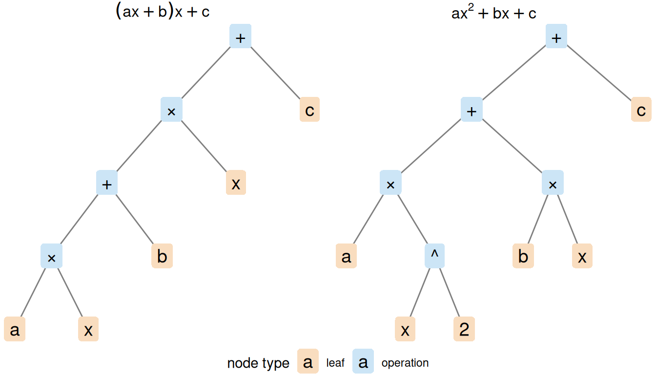
Precedence parses $a x^2 + b x + c$ as a sum of three terms: the power $x^2$ is applied first, then $a$ multiplies $x^2$ and $b$ multiplies $x$, and the three products are added. The parentheses in $(a x + b)\,x + c$ force a different tree: $a$ multiplies $x$, $b$ is added, the sum multiplies $x$, and $c$ is added.

Definition 3 (Closed-form expression (formula))

Definition 3 (Closed-form expression (formula)) A closed-form expression (or formula) [2] is an expression built from constants and variables using a finite number of operations from a list of accepted functions, such as powers, roots, exponentials, logarithms, and trigonometric functions. Which functions are accepted is a convention, and a source states it when the boundary matters.

Example 2 (The quadratic formula)

Example 2 (The quadratic formula) For $a \neq 0$ with $b^2 - 4 a c \ge 0$, the roots of $a x^2 + b x + c = 0$ are

\[ x = \frac{-b \pm \sqrt{b^2 - 4 a c}}{2 a}, \]

where the right-hand side is a closed-form expression in $a$, $b$, and $c$. By contrast, no closed-form expression is known for the root of $x - \cos x = 0$.

Definition 4 (Closed-form solution)

Definition 4 (Closed-form solution) A closed-form solution of a problem, such as solving an equation or minimizing a function, is a closed-form expression for the answer.

Example 3 (Least squares versus logistic regression)

Example 3 (Least squares versus logistic regression) Minimizing the squared-error cost of a linear model over $\mathord{\smash[b]{\underset{\raise.3ex\hbox{$\scriptstyle\sim$}}{\beta}}\vphantom{\beta}}$ gives the normal equations ${D}^{\top} D \mathord{\smash[b]{\underset{\raise.3ex\hbox{$\scriptstyle\sim$}}{\beta}}\vphantom{\beta}}= {D}^{\top} \mathord{\smash[b]{\underset{\raise.3ex\hbox{$\scriptstyle\sim$}}{y}}\vphantom{y}}$. When ${D}^{\top} D$ is invertible, the unique minimizer is

\[ \hat{\mathord{\smash[b]{\underset{\raise.3ex\hbox{$\scriptstyle\sim$}}{\beta}}\vphantom{\beta}}}= {\mathopen{}\left({D}^{\top} D\right)\mathclose{}}^{-1} {D}^{\top} \mathord{\smash[b]{\underset{\raise.3ex\hbox{$\scriptstyle\sim$}}{y}}\vphantom{y}}, \]

whose right-hand side is a closed-form expression, so least squares has a closed-form solution.

For logistic regression, no closed-form expression is known for a minimizer of the negative log-likelihood over $\mathord{\smash[b]{\underset{\raise.3ex\hbox{$\scriptstyle\sim$}}{\beta}}\vphantom{\beta}}$, so that problem has no known closed-form solution. When a minimizer exists, an iterative method approximates it.

Definition 5 (Parse tree)

Definition 5 (Parse tree) The parse tree [3] of an expression is the tree that shows how its symbols group into operations. Its leaves are the constants and variables of the expression, and each internal node is an operation applied to the nodes below it.

Example 4 (The parse tree of a polynomial)

Example 4 (The parse tree of a polynomial) The parse tree of $(a x + b)\,x + c$, with each operation having two children, is drawn in Figure 1 (left) and written out as a list here:

the root $+$, whose children are
- the node $\times$, whose children are
  - the node $+$, whose children are
    - the node $\times$, whose children are the leaves $a$ and $x$,
    - the leaf $b$;
  - the leaf $x$;
- the leaf $c$.

Read from the leaves up, the tree says to multiply $a$ by $x$, add $b$, multiply by $x$, and add $c$. The expression $a x^2 + b x + c$ has a different tree (Figure 1, right). Its root is the $+$ whose children are $a x^2 + b x$ and $c$, and the first of these is a $+$ whose children are $a x^2$ and $b x$.

Show R code

# Each tree is a nested list: the first element is the node's label,
# and the remaining elements are its children.
times <- intToUtf8(215)
trees <- list(
  "(a * x + b) * x + c" = list(
    "+",
    list(times, list("+", list(times, "a", "x"), "b"), "x"),
    "c"
  ),
  "a * x^2 + b * x + c" = list(
    "+",
    list(
      "+",
      list(times, "a", list("^", "x", "2")),
      list(times, "b", "x")
    ),
    "c"
  )
)

# Leaves sit at consecutive x positions;
# each operation sits above the mean of its children.
layout_tree <- function(node, depth = 0, next_x = 0) {
  if (!is.list(node)) {
    return(list(
      nodes = data.frame(label = node, x = next_x, y = -depth, is_leaf = TRUE),
      edges = NULL,
      next_x = next_x + 1
    ))
  }
  nodes <- NULL
  edges <- NULL
  child_x <- numeric()
  for (child in node[-1]) {
    sub <- layout_tree(child, depth + 1, next_x)
    next_x <- sub$next_x
    child_x <- c(child_x, sub$nodes$x[1])
    edges <- rbind(
      edges,
      sub$edges,
      data.frame(
        x = NA_real_,
        y = -depth,
        xend = sub$nodes$x[1],
        yend = sub$nodes$y[1]
      )
    )
    nodes <- rbind(nodes, sub$nodes)
  }
  me <- data.frame(
    label = node[[1]],
    x = mean(child_x),
    y = -depth,
    is_leaf = FALSE
  )
  edges$x[is.na(edges$x)] <- me$x
  list(nodes = rbind(me, nodes), edges = edges, next_x = next_x)
}

laid_out <- lapply(trees, layout_tree)
tree_nodes <- do.call(rbind, Map(
  function(res, name) cbind(res$nodes, tree = name),
  laid_out,
  names(trees)
))
tree_edges <- do.call(rbind, Map(
  function(res, name) cbind(res$edges, tree = name),
  laid_out,
  names(trees)
))
tree_nodes$kind <- ifelse(tree_nodes$is_leaf, "leaf", "operation")
tree_nodes$tree <- factor(tree_nodes$tree, levels = names(trees))
tree_edges$tree <- factor(tree_edges$tree, levels = names(trees))

ggplot2::ggplot() +
  ggplot2::geom_segment(
    data = tree_edges,
    ggplot2::aes(x = x, y = y, xend = xend, yend = yend),
    colour = "grey50"
  ) +
  ggplot2::geom_label(
    data = tree_nodes,
    ggplot2::aes(x = x, y = y, label = label, fill = kind),
    size = 5,
    linewidth = 0
  ) +
  ggplot2::scale_fill_manual(
    values = c(operation = "#CCE5F6", leaf = "#F9DDBF")
  ) +
  ggplot2::facet_wrap(
    ~tree,
    scales = "free_x",
    labeller = ggplot2::label_parsed
  ) +
  ggplot2::labs(fill = "node type") +
  ggplot2::theme_void() +
  ggplot2::theme(
    legend.position = "bottom",
    strip.text = ggplot2::element_text(size = 12)
  )

Two parse trees, drawn with the root at the top. In the left tree the root plus has children times and the leaf c. That times has children plus and the leaf x. The plus below it has children times and the leaf b, and that times has the leaves a and x. In the right tree the root plus has children plus and the leaf c. That plus has two children, both times. The first times has the leaf a and a power node with leaves x and 2. The second times has the leaves b and x. — Figure 1: The parse trees of $(a x + b)\,x + c$ and $a x^2 + b x + c$. Each operation is a node with one child per argument, and the leaves are the symbols that are not operations. The caret is the power operation, which takes a base and an exponent.

Remark 1 (Expressions, precedence and parse trees)

Remark 1 (Expressions, precedence and parse trees). An expression does not say how to compute the output it fixes, and many expressions denote the same function. A function is the input-output relationship itself; an expression is one way of writing it down.

The rules of operator precedence (PEMDAS: parentheses, exponents, multiplication and division, addition and subtraction) decide how the symbols group. They turn the string into its parse tree (Definition 5).

2 Algorithms

Definition 6 (Algorithm)

Definition 6 (Algorithm) An algorithm [4] is a finite list of unambiguous steps that, applied to any valid input, halts and returns an output.

Definition 7 (Computes)

Definition 7 (Computes) An algorithm computes a function when, for each input, it returns the function’s value at that input.

Example 5 (Two algorithms for one function)

Example 5 (Two algorithms for one function) Take the function that Example 1 writes two ways. Evaluating the tree of $a x^2 + b x + c$, with $x^2$ computed as $x \cdot x$, takes three multiplications and two additions. Evaluating the tree of Horner’s form $(a x + b)\,x + c$ takes two multiplications and two additions. We evaluate both forms at $a = 2$, $b = -3$, $c = 5$ and $x = 1.5$, in R and in Python, and give each intermediate quantity a name. (The code calls $c$ c0, because c is a built-in function in R.) The two algorithms compute the same function, so the two values must agree.

R
Python

a <- 2
b <- -3
c0 <- 5
x <- 1.5
# Expanded form: 3 multiplications, 2 additions
square_term <- a * x * x
linear_term <- b * x
expanded <- square_term + linear_term + c0
# Horner's form: 2 multiplications, 2 additions
inner <- a * x + b
horner <- inner * x + c0
c(square_term, linear_term, expanded)
#> [1]  4.5 -4.5  5.0
c(inner, horner)
#> [1] 0 5

a = 2
b = -3
c0 = 5
x = 1.5
# Expanded form: 3 multiplications, 2 additions
square_term = a * x * x
linear_term = b * x
expanded = square_term + linear_term + c0
# Horner's form: 2 multiplications, 2 additions
inner = a * x + b
horner = inner * x + c0
print(square_term, linear_term, expanded)
#> 4.5 -4.5 5.0
print(inner, horner)
#> 0.0 5.0

The expanded form adds 4.5, -4.5 and 5 to reach 5. Horner’s form multiplies 0 by 1.5 and adds 5 to reach 5. Different steps give the same value.

Remark 2 (Procedures that are not algorithms here)

Remark 2 (Procedures that are not algorithms here). By the definition of an algorithm, every algorithm computes some function. That holds because an algorithm has unambiguous steps and halts on every valid input. A procedure that makes random choices can return different values for the same input. A procedure that never halts returns no value for some inputs. Neither computes a function, and neither is an algorithm in this sense, although some texts call them algorithms.

Remark 3 (How functions, expressions and algorithms relate)

Remark 3 (How functions, expressions and algorithms relate). The three ideas fit together this way:

A function is the input-output relationship.
An expression denotes a function, and many expressions denote the same one.
An algorithm computes a function, and many algorithms compute the same one.

An expression is not an algorithm, because it does not say what to do, or in what order. Given values for its variables, evaluating its parse tree from the leaves up is one algorithm for the function it denotes, and a different expression for the same function gives a different tree and a different algorithm.

Remark 4 (Values with no known algorithm)

Remark 4 (Values with no known algorithm). Some functions have no known finite algorithm for their exact values, and expressions that denote them, such as a limit, a supremum, an integral with no closed form, or an $\arg \min$ over a set with no formula for the minimizer, cannot be evaluated by following their tree. Such a value can still be well defined and approximated by an algorithm.

Example 6 (A minimizer with no known formula)

Example 6 (A minimizer with no known formula) The minimizer $\arg \min_{x \in \mathbb{R}} \mathopen{}\left(x - \cos x\right)\mathclose{}^2$ is well defined, because $x - \cos x$ is strictly increasing and equals zero at one point, yet that point has no known closed-form expression, so no known finite list of arithmetic steps returns it exactly. An algorithm such as bisection approximates it as closely as we like.

3 Exercises

Exercise 1 (Is an expression an algorithm?)

Exercise 1 (Is an expression an algorithm?) How do a function, an expression and an algorithm differ?

Solution 1

Solution 1. A function is the input-output relationship. An expression is a string of symbols that denotes a function, and many expressions denote the same one. An algorithm is a finite list of steps that computes a function, and many algorithms compute the same one.

Exercise 2 (Is an expression an algorithm? (part 2))

Exercise 2 (Is an expression an algorithm? (part 2)) Use the setup of Exercise 1.

Which of the three does $a x^2 + b x + c$ name: a function, an expression or an algorithm?

Solution 2

Solution 2. It is an expression: it names a function, and it is not an algorithm.

Exercise 3 (Is an expression an algorithm? (part 3))

Exercise 3 (Is an expression an algorithm? (part 3)) Use the setup of Exercise 1.

Does the expression $a x^2 + b x + c$ tell you which arithmetic steps to carry out?

Solution 3

Solution 3. Not by itself. The expression says what to compute, not how to compute it. Once $a$, $b$, $c$ and $x$ are known, evaluating its parse tree from the leaves up is an algorithm.

Exercise 4 (Is an expression an algorithm? (part 4))

Exercise 4 (Is an expression an algorithm? (part 4)) Use the setup of Exercise 1.

What do the rules of precedence (PEMDAS) contribute to the expression $a x^2 + b x + c$?

Solution 4

Solution 4. Precedence resolves how the symbols group: $a x^2 + b x + c$ groups into three parts added together, with $x^2$ evaluated before the multiplication by $a$, and that grouping is a tree. Precedence is a rule for reading the expression, not a step in an algorithm that evaluates it.

Exercise 5 (Is an expression an algorithm? (part 5))

Exercise 5 (Is an expression an algorithm? (part 5)) Use the setup of Exercise 1.

Write a second expression that denotes the same function as $a x^2 + b x + c$ and needs fewer multiplications.

Solution 5

Solution 5. $(a x + b)\,x + c$, Horner’s form. It uses two multiplications and two additions, where the first form, with $x^2$ computed as $x \cdot x$, uses three multiplications and two additions. The two expressions denote the same function and describe different algorithms.

References

[1]

Wikipedia contributors, “Expression (mathematics) — Wikipedia, the free encyclopedia.” 2026. Available: https://en.wikipedia.org/wiki/Expression_(mathematics)

[2]

Wikipedia contributors, “Closed-form expression — Wikipedia, the free encyclopedia.” 2026. Available: https://en.wikipedia.org/wiki/Closed-form_expression

[3]

Wikipedia contributors, “Parse tree — Wikipedia, the free encyclopedia.” 2026. Available: https://en.wikipedia.org/wiki/Parse_tree

[4]

Wikipedia contributors, “Algorithm — Wikipedia, the free encyclopedia.” 2026. Available: https://en.wikipedia.org/wiki/Algorithm