Calculus
1 Derivatives
ProofProof
Proof. Apply Theorem 8 and Theorem 4:
\[ \begin{aligned} \frac{d }{d x}\operatorname{log}\mathopen{}\left\{f(x)\right\}\mathclose{} &= f'(x) \cdot\operatorname{log}'\mathopen{}\left\{f(x)\right\}\mathclose{} && \text{(chain rule, with } g = f \text{ and outer function } \log \text{)} \\ &= f'(x) \cdot\frac{1}{f(x)} && \text{(derivative of } \log \text{, valid because } f(x) > 0 \text{)} \\ &= \frac{f'(x)}{f(x)} && \text{(multiply)} \end{aligned} \]
2 Integration
Integration is the inverse operation of differentiation: it recovers a function from its derivative and accumulates quantities such as areas, totals, and probabilities. We begin with antiderivatives, then state basic integration rules, and conclude with the Fundamental Theorem of Calculus and a worked example from probability.
2.1 Antiderivatives
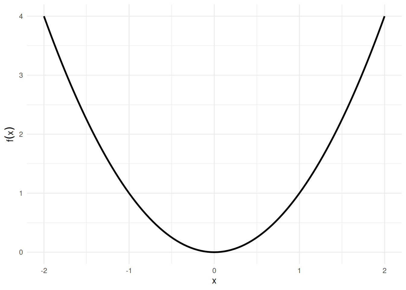
Example 1 (Antiderivative of a power function) For \(f(x) = x^2\), an antiderivative is \(F(x) = \frac{x^3}{3}\), since \(\frac{\partial}{\partial x}\frac{x^3}{3} = x^2 = f(x)\).
Adding any constant \(C\) gives another antiderivative; for example, with \(C = 7\), \(F(x) = \frac{x^3}{3} + 7\) also satisfies \(F'(x) = x^2\), since adding a constant does not change the derivative. See Figure 1.
Show R code
ggplot2::ggplot() +
  ggplot2::geom_function(fun = \(x) x^2, xlim = x_lim, linewidth = 1) +
  ggplot2::labs(x = "x", y = expression(f(x))) +
ggplot2::theme_minimal()Show R code
x_seq <- seq(x_lim[1], x_lim[2], length.out = 200)
df <- do.call(rbind, lapply(C_vals, \(C) {
  data.frame(
    x = x_seq,
    y = x_seq^3 / 3 + C,
    C = factor(C)
  )
}))

ggplot2::ggplot(df, ggplot2::aes(x = x, y = y, color = C)) +
  ggplot2::geom_line(linewidth = 0.8) +
  ggplot2::labs(x = "x", y = expression(F(x)), color = "C") +
  ggplot2::theme_minimal()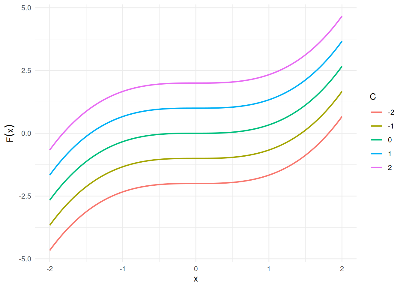
2.2 Regularity Conditions
Before stating the Fundamental Theorem of Calculus, we record two prerequisite results. The usual statement of the Fundamental Theorem of Calculus assumes that the integrand \(f\) is continuous on \([a, b]\); continuity is sufficient there, though not necessary. The two results are “differentiability implies continuity”, which says where continuity comes from, and “continuity implies integrability”, which says what continuity buys us.
ProofProof
Proof. Because \(f'(c)\) exists, \(f(c)\) is defined, and:
\[ \begin{aligned} \lim_{h \to 0} \mathopen{}\left(f(c + h) - f(c)\right)\mathclose{} &= \lim_{h \to 0} \mathopen{}\left(\frac{f(c + h) - f(c)}{h} \cdot h\right)\mathclose{} && \text{(multiply and divide by } h \neq 0 \text{)} \\ &= \mathopen{}\left(\lim_{h \to 0} \frac{f(c + h) - f(c)}{h}\right)\mathclose{} \cdot\mathopen{}\left(\lim_{h \to 0} h\right)\mathclose{} && \text{(limit of a product, both limits exist)} \\ &= f'(c) \cdot 0 && \text{(definition of } f'(c) \text{)} \\ &= 0 && \text{(multiply)} \end{aligned} \]
So \(\lim_{h \to 0} f(c + h) = f(c)\), which is \(\lim_{x \to c} f(x) = f(c)\) with \(x = c + h\); all three conditions of Definition 5 hold.
Example 8 (Continuous but not differentiable: \(\mathopen{}\left|x\right|\mathclose{}\)) The absolute-value function \(f(x) = \mathopen{}\left|x\right|\mathclose{}\) is continuous at \(x = 0\) (\(\lim_{x \to 0}\mathopen{}\left|x\right|\mathclose{} = 0 = \mathopen{}\left|0\right|\mathclose{}\)), but it is not differentiable at \(x = 0\): the left-derivative is \(-1\) and the right-derivative is \(+1\).
This counterexample shows that the converse of Theorem 10 fails: continuity does not imply differentiability. See Figure 2.
Show R code
ggplot2::ggplot() +
  ggplot2::geom_function(fun = abs, xlim = c(-2, 2), linewidth = 1) +
  ggplot2::geom_point(ggplot2::aes(x = 0, y = 0), size = 3) +
  ggplot2::labs(x = "x", y = expression(f(x) == abs(x))) +
  ggplot2::theme_minimal()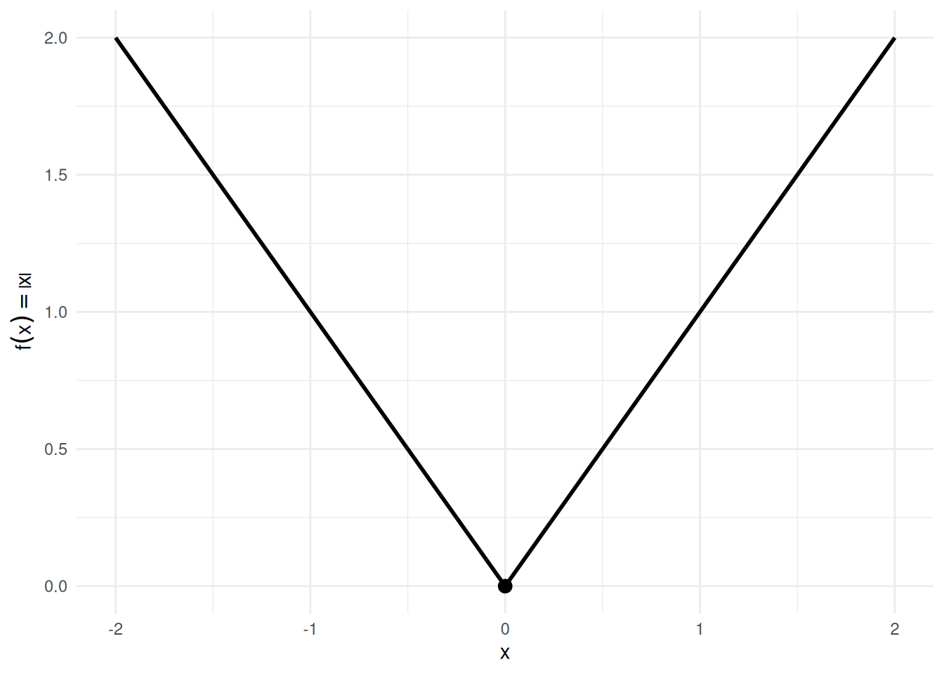
Example 10 (Integrable but not continuous: a step function) Let \(f(x) = 0\) for \(x < \tfrac{1}{2}\) and \(f(x) = 1\) for \(x \ge \tfrac{1}{2}\). Then \(f\) is discontinuous at \(x = \tfrac{1}{2}\), but it is integrable on \([0, 1]\):
\[ \int_0^1 f(x)\,dx = \int_0^{1/2} 0\,dx + \int_{1/2}^1 1\,dx = 0 + \tfrac{1}{2} = \tfrac{1}{2}. \]
This counterexample shows that the converse of Theorem 11 fails: integrability does not imply continuity. See Figure 3.
Show R code
step_df <- data.frame(
  x = c(0, 0.5, 0.5, 1),
  y = c(0, 0, 1, 1),
  segment = c("left", "left", "right", "right")
)

ggplot2::ggplot() +
  ggplot2::geom_rect(
    ggplot2::aes(xmin = 0.5, xmax = 1, ymin = 0, ymax = 1),
    fill = "steelblue", alpha = 0.3
  ) +
  ggplot2::geom_line(
    data = step_df,
    ggplot2::aes(x = x, y = y, group = segment),
    linewidth = 1
  ) +
  ggplot2::geom_point(ggplot2::aes(x = 0.5, y = 0), shape = 1, size = 3) +
  ggplot2::geom_point(ggplot2::aes(x = 0.5, y = 1), shape = 16, size = 3) +
  ggplot2::scale_x_continuous(
    breaks = c(0, 0.5, 1),
    labels = c("0", "1/2", "1")
  ) +
  ggplot2::scale_y_continuous(limits = c(-0.1, 1.2)) +
  ggplot2::labs(x = "x", y = "f(x)") +
  ggplot2::theme_minimal()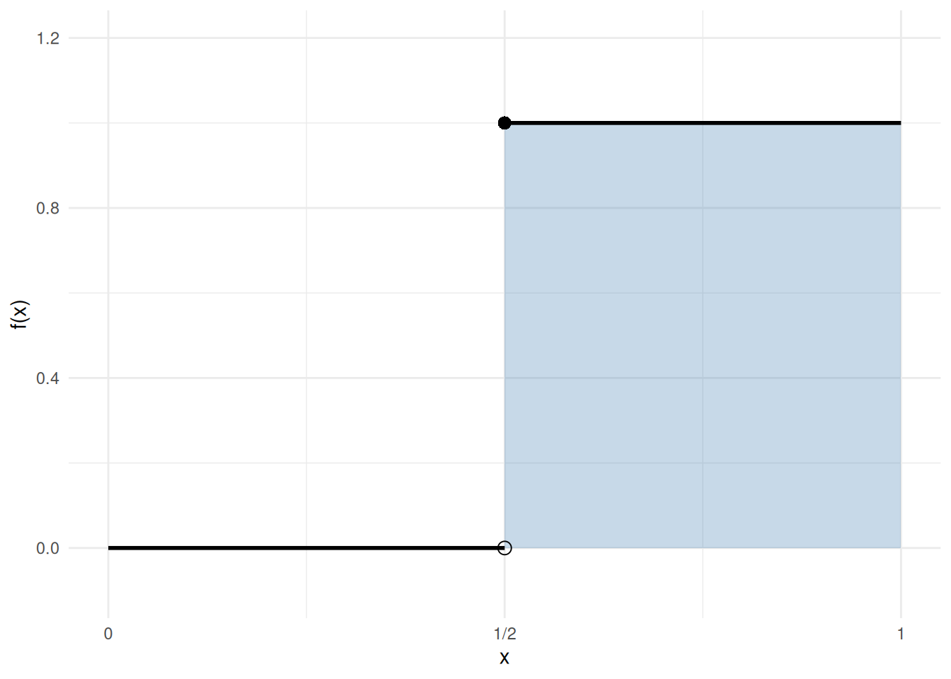
Together, Theorem 10 and Theorem 11 establish the chain:
\[\text{differentiable on } [a, b] \;\Rightarrow\; \text{continuous on } [a, b] \;\Rightarrow\; \text{integrable on } [a, b]\]
Example 8 and Example 10 show that neither implication reverses in general.
ProofProof
Proof. The \(n\) equal-width subintervals form a partition of \([a, b]\) whose mesh (Definition 8) is \((b - a)/n\), which goes to \(0\) as \(n \to \infty\). So \(S_n\) is one of the sums in the limit that defines the integral (Definition 9), along a sequence of partitions whose mesh goes to \(0\), and a limit that has the same value for every choice of partitions has that value along this sequence too.
2.3 Fundamental Theorem of Calculus
The two parts of the FTC together express that differentiation and integration are inverse operations:
- Part 1: differentiating the integral of \(f\) recovers \(f\) (Equation 1).
- Part 2: the integral of \(f\) over \([a, b]\) equals the difference of any antiderivative’s values at the endpoints (Equation 2), which rearranges to “integrating the derivative of \(F\) recovers the net change in \(F\)” (Equation 3).
The standard form of the FTC assumes \(f\) is continuous on \([a, b]\); continuity is sufficient but not strictly necessary (see the callout note inside Theorem 13 for the more general statement). Since differentiability implies continuity (Theorem 10), the FTC applies in particular whenever \(f\) is differentiable — a common situation in applied statistics.
Example 12 (FTC Part 1 visualized: accumulation function for \(f(t) = 2t\)) Take \(f(t) = 2t\) on \([0, 2]\). The accumulation function from \(0\) is
\[F(x) \;\stackrel{\text{def}}{=}\; \int_0^x 2t\,dt \;=\; \mathopen{}\left[t^2\right]\mathclose{}_{t=0}^{t=x} \;=\; x^2 - 0^2 \;=\; x^2,\]
so \(F(x) = x^2\), and indeed \(F'(x) = 2x = f(x)\), as Theorem 13 Part 1 predicts. Figure 4 shows the integrand on the left (shaded area equals \(F(x)\) at each \(x\)) and the accumulation function \(F(x) = x^2\) on the right (its slope at \(x\) equals \(f(x) = 2x\)).
Show R code
ggplot2::ggplot() +
  ggplot2::geom_area(
    data = data.frame(t = seq(0, x_focus, length.out = 200)),
    ggplot2::aes(x = t, y = 2 * t),
    fill = "steelblue", alpha = 0.4
  ) +
  ggplot2::geom_function(fun = \(t) 2 * t, xlim = c(0, 2.2), linewidth = 1) +
  ggplot2::geom_vline(
    data = data.frame(x = x_marks),
    ggplot2::aes(xintercept = x, color = factor(x)),
    linetype = "dashed", linewidth = 0.6
  ) +
  ggplot2::labs(x = "t", y = "f(t) = 2t", color = "x") +
  ggplot2::theme_minimal() +
  ggplot2::theme(legend.position = "bottom")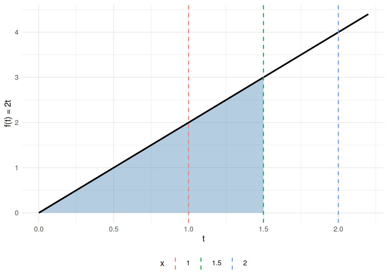
Show R code
slope_df <- data.frame(
  x = x_marks,
  Fx = x_marks^2,
  slope = 2 * x_marks
)

ggplot2::ggplot() +
  ggplot2::geom_function(fun = \(x) x^2, xlim = c(0, 2.2), linewidth = 1) +
  ggplot2::geom_point(
    data = slope_df,
    ggplot2::aes(x = x, y = Fx, color = factor(x)),
    size = 3
  ) +
  ggplot2::geom_segment(
    data = slope_df,
    ggplot2::aes(
      x = x - 0.3, xend = x + 0.3,
      y = Fx - 0.3 * slope, yend = Fx + 0.3 * slope,
      color = factor(x)
    ),
    linewidth = 0.8
  ) +
  ggplot2::labs(x = "x", y = expression(F(x) == x^2), color = "x") +
  ggplot2::theme_minimal() +
  ggplot2::theme(legend.position = "bottom")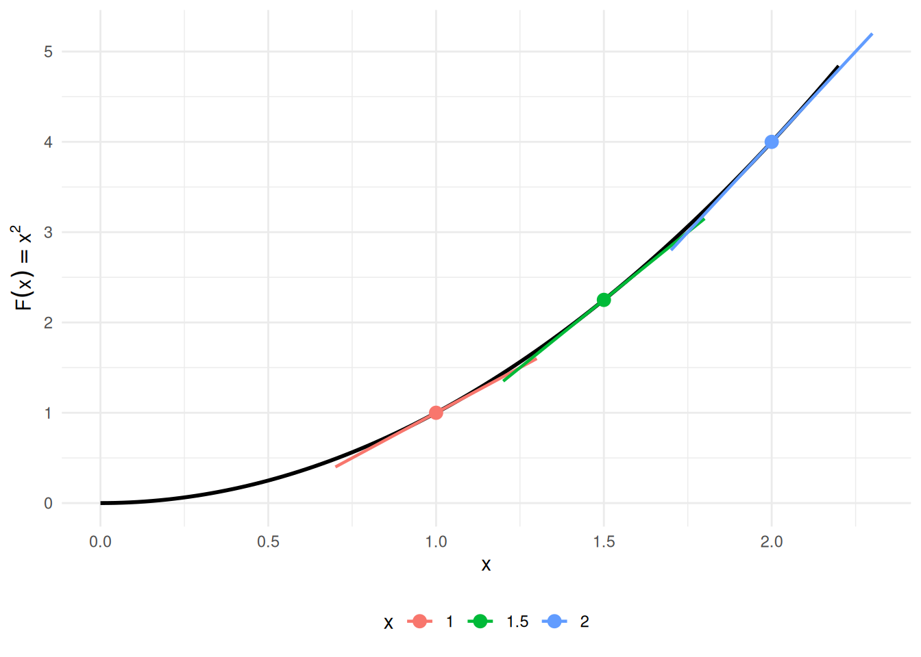
Example 13 (CDF and PDF of the exponential distribution) In what follows, \(f\) denotes the PDF and \(F\) the CDF — the same letters as the antiderivative pair in Definition 1, because the FTC will show \(F\) is exactly an antiderivative of \(f\).
Let \(T\) be a random variable with the exponential distribution with rate parameter \(\lambda > 0\). Its probability density function (PDF) is (Kleinbaum and Klein 2012, sec. II, p. 295, “Survival and Hazard Functions for Selected Distributions”):
\[f(t) = \lambda \text{e}^{-\lambda t}, \quad t \ge 0\]
FTC Part 2 gives the cumulative distribution function (CDF), \(F(t) = P(T \le t)\), from the PDF. Apply the \(\text{e}^{cx}\) rule from Theorem 9 with \(c = -\lambda\) to antidifferentiate the integrand:
\[ \begin{aligned} F(t) &= \int_0^t \lambda \text{e}^{-\lambda u}\,du && \text{(the CDF integrates the PDF)} \\ &= \mathopen{}\left[\lambda \cdot\frac{1}{-\lambda}\text{e}^{-\lambda u}\right]\mathclose{}_{u=0}^{u=t} && \text{(FTC Part 2, with the } \text{e}^{cx} \text{ rule)} \\ &= \mathopen{}\left[(-1)\text{e}^{-\lambda u}\right]\mathclose{}_{u=0}^{u=t} && \text{(} \lambda / (-\lambda) = -1 \text{)} \\ &= \mathopen{}\left[-\text{e}^{-\lambda u}\right]\mathclose{}_{u=0}^{u=t} && \text{(multiply by } -1 \text{)} \\ &= -\text{e}^{-\lambda t} - \mathopen{}\left(-\text{e}^{0}\right)\mathclose{} && \text{(evaluate at the limits)} \\ &= -\text{e}^{-\lambda t} - (-1) && \text{(} \text{e}^{0} = 1 \text{)} \\ &= 1 - \text{e}^{-\lambda t} && \text{(rearrange)} \end{aligned} \]
FTC Part 1 recovers the PDF from the CDF:
\[ \begin{aligned} \frac{\partial}{\partial t} F(t) &= \frac{\partial}{\partial t}\mathopen{}\left(1 - \text{e}^{-\lambda t}\right)\mathclose{} && \text{(substitute } F \text{)} \\ &= \frac{\partial}{\partial t} 1 - \frac{\partial}{\partial t} \text{e}^{-\lambda t} && \text{(derivative of a difference)} \\ &= 0 - \frac{\partial}{\partial t} \text{e}^{-\lambda t} && \text{(constant rule)} \\ &= 0 - \text{e}^{-\lambda t} \cdot\frac{\partial}{\partial t}(-\lambda t) && \text{(chain rule, with inner function } -\lambda t \text{)} \\ &= 0 - \text{e}^{-\lambda t} \cdot(-\lambda) && \text{(constant multiple rule)} \\ &= \lambda\text{e}^{-\lambda t} && \text{(simplify)} \\ &= f(t) && \text{(definition of } f \text{)} \end{aligned} \]
For a concrete instance: with \(\lambda = 1\) (standard exponential), the probability that \(T \le 2\) is:
\[ F(2) = 1 - \text{e}^{-1 \cdot 2} = 1 - \text{e}^{-2} \approx 1 - 0.135 = 0.865 \]
See Figure 5.
Show R code
ggplot2::ggplot() +
  ggplot2::geom_area(
    data = data.frame(t = seq(0, t_focus, length.out = 300)),
    ggplot2::aes(x = t, y = lambda * exp(-lambda * t)),
    fill = "steelblue", alpha = 0.4
  ) +
  ggplot2::geom_function(
    fun = \(t) lambda * exp(-lambda * t),
    xlim = c(0, t_max), linewidth = 1
  ) +
  ggplot2::labs(x = "t", y = "f(t)") +
  ggplot2::theme_minimal()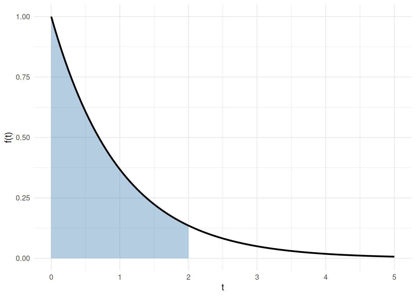
Show R code
ggplot2::ggplot() +
  ggplot2::geom_function(
    fun = \(t) 1 - exp(-lambda * t),
    xlim = c(0, t_max), linewidth = 1
  ) +
  ggplot2::geom_point(
    ggplot2::aes(x = t_focus, y = F_at_focus),
    size = 3, color = "steelblue"
  ) +
  ggplot2::geom_segment(
    ggplot2::aes(x = t_focus, xend = t_focus, y = 0, yend = F_at_focus),
    linetype = "dashed", color = "steelblue"
  ) +
  ggplot2::geom_segment(
    ggplot2::aes(x = 0, xend = t_focus, y = F_at_focus, yend = F_at_focus),
    linetype = "dashed", color = "steelblue"
  ) +
  ggplot2::labs(x = "t", y = "F(t)") +
  ggplot2::theme_minimal()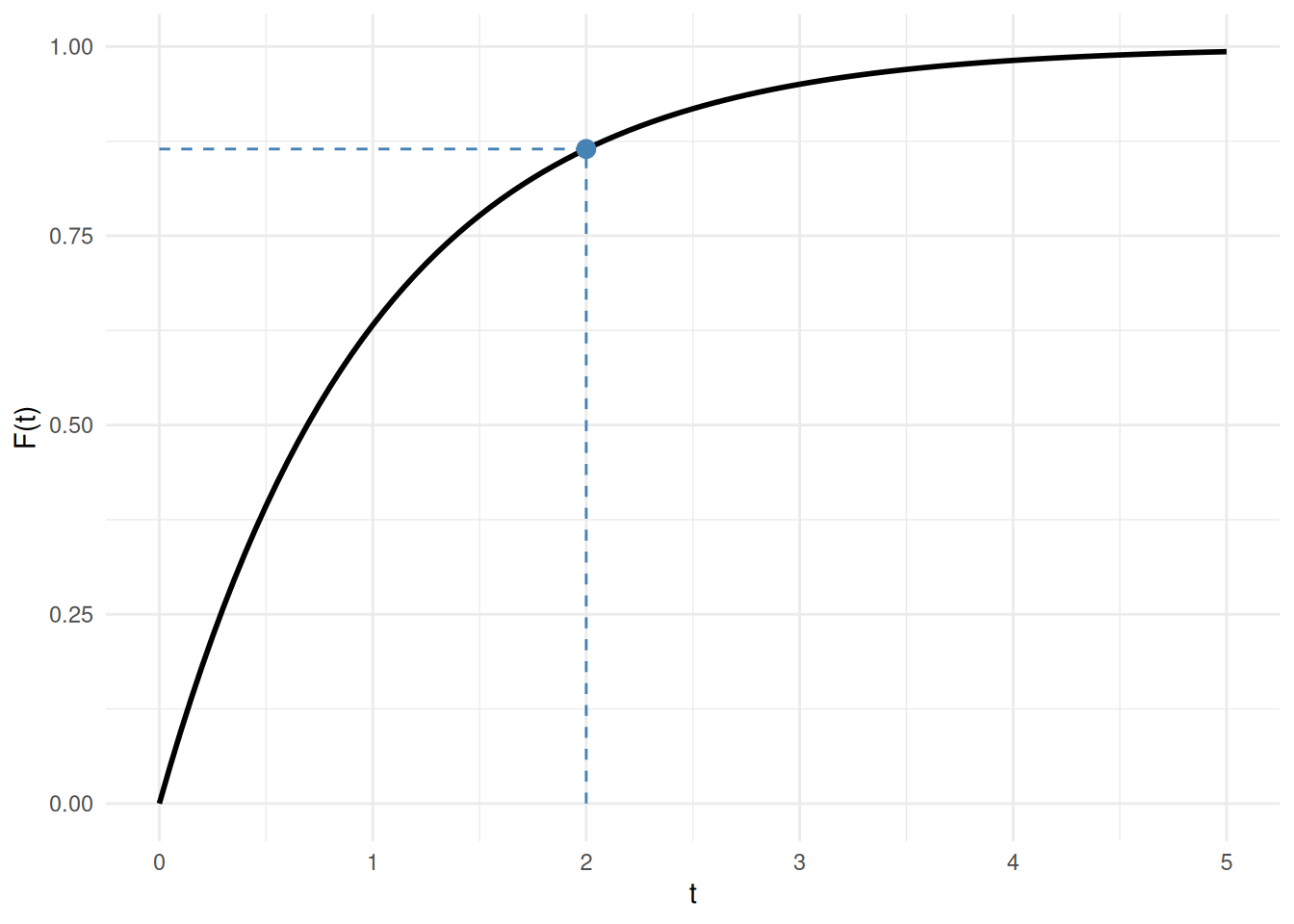
3 Double Integrals
The Fubini–Tonelli theorem states conditions under which the order of integration in a double integral can be exchanged. We state two versions: the Riemann version (Theorem 14) is what applied courses usually use for double integrals of continuous functions on simple regions; the \(\sigma\)-finite measure-theoretic version (Theorem 15) is included to make the joint-distribution form corollary in the probability chapter of Regression Models for Epidemiology follow from a stated theorem rather than from an aside.
The symbol \(dA\) stands for an element of area. An iterated integral such as \(\int_a^b \int_c^d f(x, y)\,dy\,dx\) means \(\int_a^b \mathopen{}\left(\int_c^d f(x, y)\,dy\right)\mathclose{}\,dx\): integrate over the inner variable (\(y\)) first, holding the outer variable (\(x\)) fixed.
Example 15 (Changing the order of integration for a non-rectangular region) Adapted from (Larson and Edwards 2018, sec. 14.2, Example 4, pp. 984–985).
Let \(X\) and \(Y\) be independent \(\operatorname{Uniform}(0, 1)\) random variables, with joint density \(f(x, y) = 1\) on the unit square \([0, 1]^2\). Define the function \(g(x, y) = \text{e}^{-x^2}\,\mathbb{1}\mathopen{}\left(y \le x\right)\mathclose{}\), and compute its expectation \(\operatorname{E}\mathopen{}\left[g(X, Y)\right]\mathclose{}\).
Because the joint density equals \(1\) on \([0, 1]^2\), this expectation is the double integral of \(g\) over the unit square:
\[\operatorname{E}\mathopen{}\left[g(X, Y)\right]\mathclose{} = \iint_{[0, 1]^2} g(x, y)\,dA.\]
The indicator factor \(\mathbb{1}\mathopen{}\left(y \le x\right)\mathclose{}\) equals \(1\) on the triangular region where \(y \le x\) and \(0\) elsewhere, so only that region, namely \(D = \{(x, y) : x \in [0, 1],\; y \in [0, x]\}\) (Figure 6), contributes, and there \(g(x, y) = \text{e}^{-x^2}\):
\[\operatorname{E}\mathopen{}\left[g(X, Y)\right]\mathclose{} = \iint_D \text{e}^{-x^2}\,dA.\]
Show R code
region <- data.frame(x = c(0, 1, 1), y = c(0, 0, 1))
ggplot2::ggplot(region, ggplot2::aes(x = x, y = y)) +
  ggplot2::geom_polygon(
    fill = "steelblue", alpha = 0.4, color = "black", linewidth = 0.7
  ) +
  ggplot2::annotate(
    "text", x = 0.65, y = 0.28, label = "D", size = 8, fontface = "italic"
  ) +
  ggplot2::annotate(
    "text", x = 0.36, y = 0.52, label = "y == x",
    parse = TRUE, angle = 45
  ) +
  ggplot2::annotate(
    "text", x = 1.08, y = 0.5, label = "x == 1",
    parse = TRUE, angle = 90, hjust = 0.5
  ) +
  ggplot2::annotate(
    "text", x = 0.5, y = -0.1, label = "y == 0", parse = TRUE
  ) +
  ggplot2::scale_x_continuous(breaks = c(0, 0.5, 1), limits = c(-0.1, 1.3)) +
  ggplot2::scale_y_continuous(breaks = c(0, 0.5, 1), limits = c(-0.2, 1.2)) +
  ggplot2::coord_equal() +
  ggplot2::labs(x = "x", y = "y") +
  ggplot2::theme_minimal()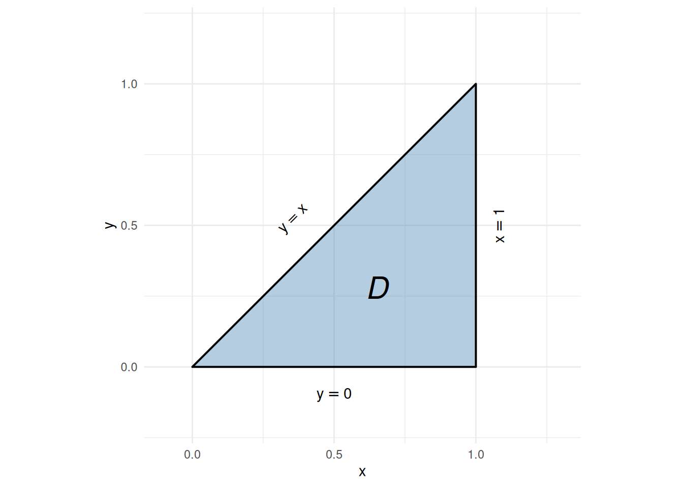
Order \(dx\,dy\) is intractable. Re-describing \(D\) as \(D = \{(x, y) : y \in [0, 1],\; x \in [y, 1]\}\), the inner integral is
\[\int_y^1 \text{e}^{-x^2}\,dx,\]
which has no elementary antiderivative.
Order \(dy\,dx\) works. Applying Theorem 14 Part 1 (\(\text{e}^{-x^2}\) is continuous and \(D\) is the vertically simple region \(x \in [0, 1]\), \(y \in [0, x]\)):
\[ \begin{aligned} \iint_D \text{e}^{-x^2}\,dA &= \int_0^1\!\int_0^x \text{e}^{-x^2}\,dy\,dx && \text{(Fubini, vertically simple region)} \\&= \int_0^1 \text{e}^{-x^2}\mathopen{}\left(\int_0^x dy\right)\mathclose{}\,dx && \text{(} \text{e}^{-x^2} \text{ is constant in } y \text{)} \\&= \int_0^1 x\,\text{e}^{-x^2}\,dx && \text{(} \textstyle\int_0^x dy = x \text{)} \end{aligned} \]
To antidifferentiate \(x\,\text{e}^{-x^2}\), let \(u = x^2\) be the inner function. By the chain rule (Theorem 8), with \(\frac{d u}{d x} = 2x\),
\[ \begin{aligned} \frac{d }{d x}\mathopen{}\left(-\frac{1}{2}\,\text{e}^{-u}\right)\mathclose{} &= -\frac{1}{2}\,\text{e}^{-u} \cdot(-1) \cdot\frac{d u}{d x} && \text{(chain rule)} \\&= -\frac{1}{2}\,\text{e}^{-x^2} \cdot(-1) \cdot 2x && \text{(substitute } u = x^2 \text{ and } du/dx = 2x \text{)} \\&= x\,\text{e}^{-x^2} && \text{(multiply)} \end{aligned} \]
so \(-\frac{1}{2}\,\text{e}^{-x^2}\) is an antiderivative of \(x\,\text{e}^{-x^2}\), and
\[ \begin{aligned} \int_0^1 x\,\text{e}^{-x^2}\,dx &= \mathopen{}\left[-\frac{1}{2}\,\text{e}^{-x^2}\right]\mathclose{}_0^1 && \text{(FTC Part 2)} \\&= -\frac{1}{2}\mathopen{}\left(\text{e}^{-1} - \text{e}^{0}\right)\mathclose{} && \text{(evaluate at the limits)} \\&= -\frac{1}{2}\mathopen{}\left(\text{e}^{-1} - 1\right)\mathclose{} && \text{(} \text{e}^{0} = 1 \text{)} \\&= \frac{1 - \text{e}^{-1}}{2} && \text{(distribute } -\tfrac{1}{2} \text{)} \\&= \frac{e - 1}{2e} && \text{(multiply numerator and denominator by } e \text{)} \\&\approx 0.316 \end{aligned} \]
The solid whose volume equals this integral is shown in Figure 7.
Show R code
n_grid <- 51
x_seq <- seq(0, 1, length.out = n_grid)
y_seq <- seq(0, 1, length.out = n_grid)

z_mat <- outer(x_seq, y_seq, function(x, y) {
  z <- exp(-x^2)
  z[y > x] <- NA
  z
})

plotly::plot_ly(x = ~x_seq, y = ~y_seq, z = ~t(z_mat)) |>
  plotly::add_surface(showscale = FALSE) |>
  plotly::layout(scene = list(
    xaxis = list(title = "x"),
    yaxis = list(title = "y"),
    zaxis = list(title = "z = exp(-x^2)"),
    camera = list(eye = list(x = 1.6, y = -1.6, z = 0.8))
  ))
ProofProof
Proof. A closed bounded rectangle \([a, b] \times [c, d]\) is both vertically simple (with \(g_1 \equiv c\), \(g_2 \equiv d\)) and horizontally simple (with \(h_1 \equiv a\), \(h_2 \equiv b\)). Applying both parts of Theorem 14 to \(f\) on this rectangle gives the two iterated forms shown.
Example 17 (Evaluating a double integral on a rectangle) Structure adapted from (Larson and Edwards 2018, sec. 14.2, Example 2, pp. 982–983); the integrand \(x^2 + y^2\) is original, chosen so the integral equals \(\operatorname{E}\mathopen{}\left[g(X, Y)\right]\mathclose{}\) for \(g(x, y) = x^2 + y^2\).
Let \(X\) and \(Y\) be independent \(\operatorname{Uniform}(0, 1)\) random variables, with joint density \(f(x, y) = 1\) on the unit square \(R = \{(x, y) : x \in [0, 1],\; y \in [0, 1]\}\) (Figure 9). Define the function \(g(x, y) = x^2 + y^2\), and compute its expectation \(\operatorname{E}\mathopen{}\left[g(X, Y)\right]\mathclose{}\).
Because the joint density equals \(1\) on \(R\), this expectation is the double integral of \(g\) over \(R\):
\[\operatorname{E}\mathopen{}\left[g(X, Y)\right]\mathclose{} = \iint_R \mathopen{}\left(x^2 + y^2\right)\mathclose{}\,dA.\]
Show R code
ggplot2::ggplot() +
  ggplot2::annotate(
    "rect", xmin = 0, xmax = 1, ymin = 0, ymax = 1,
    fill = "steelblue", alpha = 0.4, color = "black", linewidth = 0.7
  ) +
  ggplot2::annotate(
    "text", x = 0.5, y = 0.5, label = "R", size = 8, fontface = "italic"
  ) +
  ggplot2::scale_x_continuous(breaks = c(0, 1), limits = c(-0.15, 1.25)) +
  ggplot2::scale_y_continuous(breaks = c(0, 1), limits = c(-0.15, 1.25)) +
  ggplot2::coord_equal() +
  ggplot2::labs(x = "x", y = "y") +
  ggplot2::theme_minimal()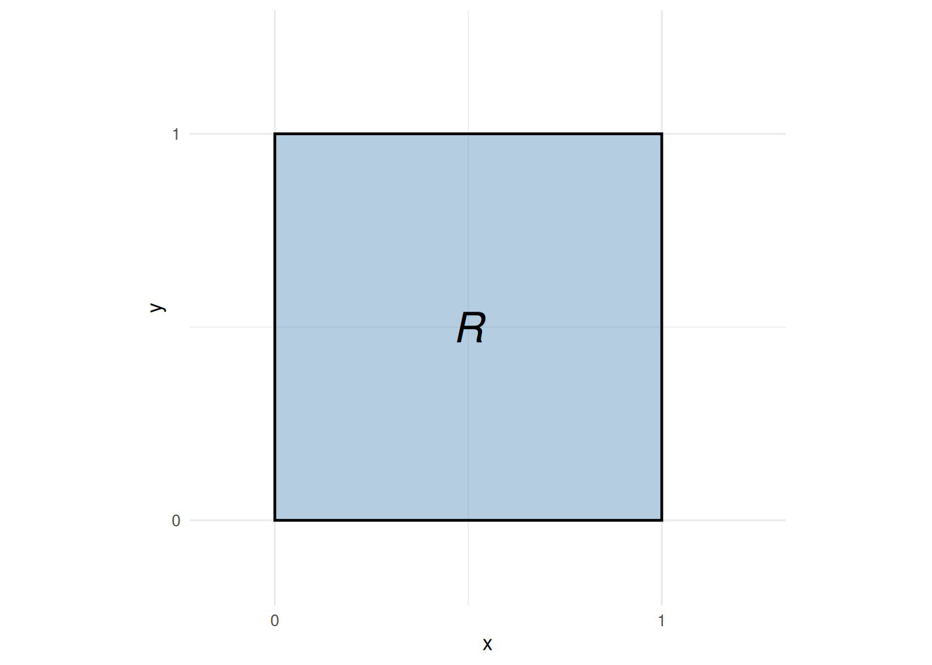
The integrand is continuous on \(R\), so Corollary 2 applies and either order of integration yields the same value.
Integrating \(y\) first, then \(x\):
\[ \begin{aligned} \operatorname{E}\mathopen{}\left[g(X, Y)\right]\mathclose{} &= \int_0^1\!\int_0^1 \mathopen{}\left(x^2 + y^2\right)\mathclose{}\,dy\,dx \\&= \int_0^1 \mathopen{}\left[x^2 y + \frac{y^3}{3}\right]\mathclose{}_0^1\,dx \\&= \int_0^1 \mathopen{}\left(x^2 + \frac{1}{3}\right)\mathclose{}\,dx \\&= \mathopen{}\left[\frac{x^3}{3} + \frac{x}{3}\right]\mathclose{}_0^1 \\&= \frac{2}{3} \end{aligned} \]
Integrating \(x\) first, then \(y\) (verifying the order can be swapped):
\[ \begin{aligned} \int_0^1\!\int_0^1 \mathopen{}\left(x^2 + y^2\right)\mathclose{}\,dx\,dy &= \int_0^1 \mathopen{}\left[\frac{x^3}{3} + y^2 x\right]\mathclose{}_0^1\,dy \\&= \int_0^1 \mathopen{}\left(\frac{1}{3} + y^2\right)\mathclose{}\,dy \\&= \mathopen{}\left[\frac{y}{3} + \frac{y^3}{3}\right]\mathclose{}_0^1 \\&= \frac{2}{3} \end{aligned} \]
Both orders give \(\frac{2}{3}\), as Corollary 2 guarantees.
As a cross-check, linearity of expectation gives the same value: since \(\operatorname{E}\mathopen{}\left[X^2\right]\mathclose{} = \int_0^1 x^2\,dx = \frac{1}{3}\) for \(X \sim \operatorname{Uniform}(0, 1)\) (and likewise for \(Y\)),
\[\operatorname{E}\mathopen{}\left[g(X, Y)\right]\mathclose{} = \operatorname{E}\mathopen{}\left[X^2 + Y^2\right]\mathclose{} = \operatorname{E}\mathopen{}\left[X^2\right]\mathclose{} + \operatorname{E}\mathopen{}\left[Y^2\right]\mathclose{} = \frac{1}{3} + \frac{1}{3} = \frac{2}{3}.\]
The solid whose volume equals this integral is shown in Figure 10.
Show R code
n_grid <- 41
x_seq <- seq(0, 1, length.out = n_grid)
y_seq <- seq(0, 1, length.out = n_grid)
z_mat <- outer(x_seq, y_seq, function(x, y) x^2 + y^2)

plotly::plot_ly(x = ~x_seq, y = ~y_seq, z = ~t(z_mat)) |>
  plotly::add_surface(showscale = FALSE) |>
  plotly::layout(scene = list(
    xaxis = list(title = "x"),
    yaxis = list(title = "y"),
    zaxis = list(title = "z", range = c(0, 2))
))Applied courses rarely need the measure-theoretic generalization itself, but it is what justifies the joint-distribution form corollary in the probability chapter of Regression Models for Epidemiology: probability measures are finite (hence \(\sigma\)-finite), so the \(\sigma\)-finiteness condition is automatic. The integrability conditions (nonnegativity or absolute integrability) still need to be verified in each application.
4 Additional resources
References
Banner, Adrian D. 2007. The Calculus Lifesaver : All the Tools You Need to Excel at Calculus. A Princeton Lifesaver Study Guide. Princeton University Press. https://press.princeton.edu/books/paperback/9780691130880/the-calculus-lifesaver.
Billingsley, Patrick. 1995. Probability and Measure. 3rd ed. Wiley Series in Probability and Mathematical Statistics. Wiley.
Fubini, Guido. 1907. “Sugli Integrali Multipli.” Rendiconti Della Reale Accademia Dei Lincei. Classe Di Scienze Fisiche, Matematiche e Naturali 16: 608–14.
Grinberg, Raffi. 2017. The Real Analysis Lifesaver: All the Tools You Need to Understand Proofs. 1st ed. Princeton Lifesaver Study Guides. Princeton University Press. https://press.princeton.edu/books/paperback/9780691172934/the-real-analysis-lifesaver.
Gut, Allan. 2013. Probability: A Graduate Course. 2nd ed. Springer Texts in Statistics. Springer. https://doi.org/10.1007/978-1-4614-4708-5.
Kaplan, Daniel. 2022. MOSAIC Calculus. Www.mosaic-web.org. www.mosaic-web.org.
Khuri, André I. 2003. Advanced Calculus with Applications in Statistics. John Wiley & Sons. https://doi.org/10.1002/0471394882.
Kleinbaum, David G, and Mitchel Klein. 2012. Survival Analysis: A Self-Learning Text. 3rd ed. Springer. https://doi.org/10.1007/978-1-4419-6646-9.
Larson, Ron, and Bruce H. Edwards. 2018. Calculus. 11th ed. Cengage Learning. https://www.cengage.com/c/calculus-11e-larson/.
Miller, Steven J. 2016. The Probability Lifesaver: Calculus Review Problems. https://web.williams.edu/Mathematics/sjmiller/public_html/probabilitylifesaver/index.htm#:~:text=http%3A//web.williams.edu/Mathematics/sjmiller/public_html/probabilitylifesaver/supplementalchap_calcreview.pdf.
Rudin, Walter. 1976. Principles of Mathematical Analysis. 3rd ed. International Series in Pure and Applied Mathematics. McGraw-Hill.
Wikipedia contributors. 2024. Fubini’s Theorem — Wikipedia, the Free Encyclopedia. https://en.wikipedia.org/wiki/Fubini%27s_theorem.