Vector Calculus
(adapted from Fieller [1], Section 7.2)
This section covers derivatives of functions of vectors and matrices. Its linear algebra prerequisites, such as vectors, matrices, transposes, dot products, and quadratic forms, are covered in Linear Algebra.
Let \(\mathord{\smash[b]{\underset{\raise.3ex\hbox{$\scriptstyle\sim$}}{x}}\vphantom{x}}\) and \(\mathord{\smash[b]{\underset{\raise.3ex\hbox{$\scriptstyle\sim$}}{\beta}}\vphantom{\beta}}\) be column vectors of length \(p\) (see column vector and dot product).
DefDefinition 1 (Partial derivative)
Definition 1 (Partial derivative) Let \(f : \mathbb{R}^p \to \mathbb{R}\) and \(\mathord{\smash[b]{\underset{\raise.3ex\hbox{$\scriptstyle\sim$}}{x}}\vphantom{x}}= {(x_1, \ldots, x_p)}^{\top} \in \mathbb{R}^p\). The partial derivative [2] of \(f\) with respect to \(x_j\) at \(\mathord{\smash[b]{\underset{\raise.3ex\hbox{$\scriptstyle\sim$}}{x}}\vphantom{x}}\) is
\[ \frac{\partial}{\partial x_j} f(\mathord{\smash[b]{\underset{\raise.3ex\hbox{$\scriptstyle\sim$}}{x}}\vphantom{x}}) \stackrel{\text{def}}{=} \lim_{h \to 0} \frac{f(x_1, \ldots, x_j + h, \ldots, x_p) - f(x_1, \ldots, x_p)}{h}, \]
when this limit exists. It is the derivative at \(x_j\) of the one-variable function \(t \mapsto f(x_1, \ldots, t, \ldots, x_p)\), which varies the \(j\)th coordinate and holds the other coordinates fixed.
Example 1 (Partial derivatives of \(x_1^2 x_2 + 3 x_2\)) Let \(f(x_1, x_2) = x_1^2 x_2 + 3 x_2\). At \(\mathord{\smash[b]{\underset{\raise.3ex\hbox{$\scriptstyle\sim$}}{x}}\vphantom{x}}= {(1, 2)}^{\top}\),
\[ \begin{aligned} f(1, 2) &= 1 \cdot 2 + 6 \\ &= 8, \end{aligned} \]
and for \(h \ne 0\)
\[ \begin{aligned} \frac{f(1 + h, 2) - f(1, 2)}{h} &= \frac{(1 + h)^2 \cdot 2 + 6 - 8}{h} && \text{(substitute into } f \text{)} \\ &= \frac{(1 + h)^2 \cdot 2 - 2}{h} && \text{(} 6 - 8 = -2 \text{)} \\ &= \frac{(1 + 2h + h^2) \cdot 2 - 2}{h} && \text{(expand } (1 + h)^2 \text{)} \\ &= \frac{2 + 4h + 2h^2 - 2}{h} && \text{(distributive law)} \\ &= \frac{4h + 2h^2 + 2 - 2}{h} && \text{(reorder the terms)} \\ &= \frac{4h + 2h^2}{h} && \text{(} 2 - 2 = 0 \text{)} \\ &= 4 + 2h, && \text{(divide by } h \ne 0 \text{)} \end{aligned} \]
which tends to \(4\) as \(h \to 0\), so \(\frac{\partial}{\partial x_1} f(1, 2) = 4\). Holding \(x_2\) fixed and differentiating in \(x_1\) gives the same answer: \(\frac{\partial}{\partial x_1} f(\mathord{\smash[b]{\underset{\raise.3ex\hbox{$\scriptstyle\sim$}}{x}}\vphantom{x}}) = 2 x_1 x_2\), which is \(2 \cdot 1 \cdot 2 = 4\) at \({(1, 2)}^{\top}\). Holding \(x_1\) fixed instead gives \(\frac{\partial}{\partial x_2} f(\mathord{\smash[b]{\underset{\raise.3ex\hbox{$\scriptstyle\sim$}}{x}}\vphantom{x}}) = x_1^2 + 3\), which is \(1 + 3 = 4\) at \({(1, 2)}^{\top}\).
ExrExercise 1 (First-order partial derivatives)
Exercise 1 (First-order partial derivatives) Adapted from Miller [3], Question 1.1.42.
Let \(f(x, y) = x^2 y + e^x + \sin(xy)\). Find \(\frac{\partial f}{\partial x}\) and \(\frac{\partial f}{\partial y}\).
ExrExercise 2 (Partial derivatives of the normal density with respect to parameters)
Exercise 2 (Partial derivatives of the normal density with respect to parameters) Adapted from Miller [3], Question 1.1.43.
Let
\[f(x; \mu, \sigma) = \frac{1}{\sqrt{2\pi\sigma^2}}{\operatorname{exp}\mathopen{}\left\{-\frac{(x - \mu)^2}{2\sigma^2}\right\}\mathclose{}}\]
Find \(\frac{\partial f}{\partial \mu}\) and \(\frac{\partial f}{\partial \sigma}\).
LemTheorem 1 (Partial derivatives of the normal density with respect to its parameters)
Theorem 1 (Partial derivatives of the normal density with respect to its parameters) Let \(\mu\in \mathbb{R}\) and \(\sigma> 0\), and let
\[f(x; \mu, \sigma) = \frac{1}{\sqrt{2\pi\sigma^2}}{\operatorname{exp}\mathopen{}\left\{-\frac{(x - \mu)^2}{2\sigma^2}\right\}\mathclose{}}\]
Then for every \(x \in \mathbb{R}\),
\[ \begin{aligned} \frac{\partial f}{\partial \mu} &= \frac{x - \mu}{\sigma^2} f(x; \mu, \sigma) \\ \frac{\partial f}{\partial \sigma} &= \mathopen{}\left[-\frac{1}{\sigma} + \frac{(x - \mu)^2}{\sigma^3}\right]\mathclose{} f(x; \mu, \sigma) \end{aligned} \]
ProofProof
Proof. This is the solution to Exercise 2, worked in Solution 2. The argument has two steps.
- For \(\frac{\partial f}{\partial \mu}\), treat \(\sigma\) as constant. The prefactor is constant, so the chain rule on the exponential gives \(\frac{\partial f}{\partial \mu} = f(x; \mu, \sigma) \cdot\mathopen{}\left[-\frac{2(x - \mu)(-1)}{2\sigma^2}\right]\mathclose{} = \frac{x - \mu}{\sigma^2} f(x; \mu, \sigma)\).
- For \(\frac{\partial f}{\partial \sigma}\), write \(f(x; \mu, \sigma) = \frac{1}{\sqrt{2\pi}}\sigma^{-1}{\operatorname{exp}\mathopen{}\left\{-\frac{(x - \mu)^2}{2\sigma^2}\right\}\mathclose{}}\). The product rule gives one term from differentiating \(\sigma^{-1}\), namely \(-\sigma^{-1} f(x; \mu, \sigma)\), and one from the chain rule on the exponential, namely \(\frac{(x - \mu)^2}{\sigma^3} f(x; \mu, \sigma)\). Adding them gives \(\mathopen{}\left[-\frac{1}{\sigma} + \frac{(x - \mu)^2}{\sigma^3}\right]\mathclose{} f(x; \mu, \sigma)\).
ExrExercise 3 (Partial derivatives with exponential of quadratic form)
Exercise 3 (Partial derivatives with exponential of quadratic form) Adapted from Miller [3], Question 1.1.44.
Find \(\frac{\partial f}{\partial x}\) and \(\frac{\partial f}{\partial y}\) for
\[f(x, y) = x{\operatorname{exp}\mathopen{}\left\{x^2 + y^2\right\}\mathclose{}}\]
ExrExercise 4 (Using symmetry to compute partial derivatives)
Exercise 4 (Using symmetry to compute partial derivatives) Adapted from Miller [3], Question 1.1.45.
Find \(\frac{\partial f}{\partial x}\) and \(\frac{\partial f}{\partial y}\) for
\[f(x, y) = e^{xy} - \log(x^2 + y^2)\]
on \(\mathbb{R}^2 \setminus \{(0, 0)\}\).
DefDefinition 2 (Vector derivative, gradient)
Definition 2 (Vector derivative, gradient) If \(f(\mathord{\smash[b]{\underset{\raise.3ex\hbox{$\scriptstyle\sim$}}{\beta}}\vphantom{\beta}})\) is a scalar-valued function of a \(p \times 1\) vector \(\mathord{\smash[b]{\underset{\raise.3ex\hbox{$\scriptstyle\sim$}}{\beta}}\vphantom{\beta}}\), such as \(f(\mathord{\smash[b]{\underset{\raise.3ex\hbox{$\scriptstyle\sim$}}{\beta}}\vphantom{\beta}}) = \mathord{\smash[b]{\underset{\raise.3ex\hbox{$\scriptstyle\sim$}}{x}}\vphantom{x}} \cdot \mathord{\smash[b]{\underset{\raise.3ex\hbox{$\scriptstyle\sim$}}{\beta}}\vphantom{\beta}}\), then its vector derivative is the column vector of its partial derivatives (Definition 1):
\[ \frac{\partial}{\partial \mathord{\smash[b]{\underset{\raise.3ex\hbox{$\scriptstyle\sim$}}{\beta}}\vphantom{\beta}}} f(\mathord{\smash[b]{\underset{\raise.3ex\hbox{$\scriptstyle\sim$}}{\beta}}\vphantom{\beta}}) = \begin{bmatrix} \frac{\partial}{\partial \beta_{1}}f(\mathord{\smash[b]{\underset{\raise.3ex\hbox{$\scriptstyle\sim$}}{\beta}}\vphantom{\beta}}) \\ \frac{\partial}{\partial \beta_{2}}f(\mathord{\smash[b]{\underset{\raise.3ex\hbox{$\scriptstyle\sim$}}{\beta}}\vphantom{\beta}}) \\ \vdots \\ \frac{\partial}{\partial \beta_{p}}f(\mathord{\smash[b]{\underset{\raise.3ex\hbox{$\scriptstyle\sim$}}{\beta}}\vphantom{\beta}}) \end{bmatrix} \]
The vector derivative is also called the gradient [4] of \(f\) with respect to \(\mathord{\smash[b]{\underset{\raise.3ex\hbox{$\scriptstyle\sim$}}{\beta}}\vphantom{\beta}}\), written \(\nabla_{\mathord{\smash[b]{\underset{\raise.3ex\hbox{$\scriptstyle\sim$}}{\beta}}\vphantom{\beta}}} f(\mathord{\smash[b]{\underset{\raise.3ex\hbox{$\scriptstyle\sim$}}{\beta}}\vphantom{\beta}})\).
ExmExample 2 (A vector derivative)
Example 2 (A vector derivative) Let \(\mathord{\smash[b]{\underset{\raise.3ex\hbox{$\scriptstyle\sim$}}{\beta}}\vphantom{\beta}}= {(\beta_{1}, \beta_{2})}^{\top}\) and \(f(\mathord{\smash[b]{\underset{\raise.3ex\hbox{$\scriptstyle\sim$}}{\beta}}\vphantom{\beta}}) = 3 \beta_{1} + 5 \beta_{2}^2\). Then
\[ \begin{aligned} \underbrace{\frac{\partial}{\partial \mathord{\smash[b]{\underset{\raise.3ex\hbox{$\scriptstyle\sim$}}{\beta}}\vphantom{\beta}}} f(\mathord{\smash[b]{\underset{\raise.3ex\hbox{$\scriptstyle\sim$}}{\beta}}\vphantom{\beta}})}_{2 \times 1} &= \begin{bmatrix} \frac{\partial}{\partial \beta_{1}} (3 \beta_{1} + 5 \beta_{2}^2) \\ \frac{\partial}{\partial \beta_{2}} (3 \beta_{1} + 5 \beta_{2}^2) \end{bmatrix} \\ &= \begin{bmatrix} 3 \\ 10 \beta_{2} \end{bmatrix}, \end{aligned} \]
and at \(\mathord{\smash[b]{\underset{\raise.3ex\hbox{$\scriptstyle\sim$}}{\beta}}\vphantom{\beta}}= {(1, 2)}^{\top}\) the vector derivative is \({(3, 20)}^{\top}\).
TipVideo lecture
Hutchinson’s Gradients Refresher (17 min) covers gradients and partial derivatives, the ideas behind this section [5]. The login for the video site is posted on Canvas.
TipVideos
Jon Krohn’s “Calculus for Machine Learning” YouTube playlist has videos on partial derivatives:
1 Checking a gradient by its shape
The gradient always has the same shape as the input it is taken with respect to, because it holds exactly one partial derivative per component of that input:
The table is the cheapest check there is on a gradient just worked out by hand: if the shapes disagree, something went wrong. It is the shape rule of matrix multiplication again, applied to calculus.
DefDefinition 3 (Linear approximation of a function of a vector, first-order Taylor approximation of a function of a vector)
Definition 3 (Linear approximation of a function of a vector, first-order Taylor approximation of a function of a vector) Let \(f : \mathbb{R}^p \to \mathbb{R}\) have a gradient at \(\mathord{\smash[b]{\underset{\raise.3ex\hbox{$\scriptstyle\sim$}}{\beta}}\vphantom{\beta}}\). The linear approximation of \(f\) at \(\mathord{\smash[b]{\underset{\raise.3ex\hbox{$\scriptstyle\sim$}}{\beta}}\vphantom{\beta}}\) [6] (also called the first-order Taylor approximation or the first-order Taylor expansion) is the function of a step \(\mathord{\smash[b]{\underset{\raise.3ex\hbox{$\scriptstyle\sim$}}{\delta}}\vphantom{\delta}}\in \mathbb{R}^p\)
\[ \hat{f}_{\mathord{\smash[b]{\underset{\raise.3ex\hbox{$\scriptstyle\sim$}}{\beta}}\vphantom{\beta}}}(\mathord{\smash[b]{\underset{\raise.3ex\hbox{$\scriptstyle\sim$}}{\delta}}\vphantom{\delta}}) \stackrel{\text{def}}{=}f(\mathord{\smash[b]{\underset{\raise.3ex\hbox{$\scriptstyle\sim$}}{\beta}}\vphantom{\beta}}) + \nabla f(\mathord{\smash[b]{\underset{\raise.3ex\hbox{$\scriptstyle\sim$}}{\beta}}\vphantom{\beta}}) \cdot \mathord{\smash[b]{\underset{\raise.3ex\hbox{$\scriptstyle\sim$}}{\delta}}\vphantom{\delta}}. \tag{1}\]
ExmExample 3 (A linear approximation of a function of two variables)
Example 3 (A linear approximation of a function of two variables) Take \(f(\mathord{\smash[b]{\underset{\raise.3ex\hbox{$\scriptstyle\sim$}}{\beta}}\vphantom{\beta}}) = 3 \beta_{1} + 5 \beta_{2}^2\) from Example 2, whose gradient at \(\mathord{\smash[b]{\underset{\raise.3ex\hbox{$\scriptstyle\sim$}}{\beta}}\vphantom{\beta}}= {(1, 2)}^{\top}\) is \(\nabla f(\mathord{\smash[b]{\underset{\raise.3ex\hbox{$\scriptstyle\sim$}}{\beta}}\vphantom{\beta}}) = {(3, 20)}^{\top}\). At that point,
\[ \begin{aligned} f(\mathord{\smash[b]{\underset{\raise.3ex\hbox{$\scriptstyle\sim$}}{\beta}}\vphantom{\beta}}) &= 3 \cdot 1 + 5 \cdot 2^2 && \text{(substitute } \beta_{1} = 1 \text{ and } \beta_{2} = 2 \text{)} \\ &= 23, && \text{(} 3 + 20 = 23 \text{)} \end{aligned} \]
so the linear approximation at \(\mathord{\smash[b]{\underset{\raise.3ex\hbox{$\scriptstyle\sim$}}{\beta}}\vphantom{\beta}}\) is
\[ \hat{f}_{\mathord{\smash[b]{\underset{\raise.3ex\hbox{$\scriptstyle\sim$}}{\beta}}\vphantom{\beta}}}(\mathord{\smash[b]{\underset{\raise.3ex\hbox{$\scriptstyle\sim$}}{\delta}}\vphantom{\delta}}) = 23 + 3 \delta_1 + 20 \delta_2. \]
For the step \(\mathord{\smash[b]{\underset{\raise.3ex\hbox{$\scriptstyle\sim$}}{\delta}}\vphantom{\delta}}= {(0.1, 0.1)}^{\top}\), the approximation is
\[ \begin{aligned} \hat{f}_{\mathord{\smash[b]{\underset{\raise.3ex\hbox{$\scriptstyle\sim$}}{\beta}}\vphantom{\beta}}}(\mathord{\smash[b]{\underset{\raise.3ex\hbox{$\scriptstyle\sim$}}{\delta}}\vphantom{\delta}}) &= 23 + 3 \cdot 0.1 + 20 \cdot 0.1 && \text{(substitute } \delta_1 = \delta_2 = 0.1 \text{)} \\ &= 25.3, && \text{(} 23 + 0.3 + 2 = 25.3 \text{)} \end{aligned} \]
and the value of \(f\) at \(\mathord{\smash[b]{\underset{\raise.3ex\hbox{$\scriptstyle\sim$}}{\beta}}\vphantom{\beta}}+ \mathord{\smash[b]{\underset{\raise.3ex\hbox{$\scriptstyle\sim$}}{\delta}}\vphantom{\delta}}= {(1.1, 2.1)}^{\top}\) is
\[ \begin{aligned} f(\mathord{\smash[b]{\underset{\raise.3ex\hbox{$\scriptstyle\sim$}}{\beta}}\vphantom{\beta}}+ \mathord{\smash[b]{\underset{\raise.3ex\hbox{$\scriptstyle\sim$}}{\delta}}\vphantom{\delta}}) &= 3 \cdot 1.1 + 5 \cdot 2.1^2 && \text{(substitute } \beta_{1} = 1.1 \text{ and } \beta_{2} = 2.1 \text{)} \\ &= 25.35. && \text{(} 3.3 + 22.05 = 25.35 \text{)} \end{aligned} \]
The approximation misses by \(0.05\), which is \(5 \delta_2^2\), the second-order term of \(f\) that the approximation leaves out. That term is never negative, and is zero only when \(\delta_2 = 0\), so the graph of the approximation in Figure 1 is a plane that touches the graph of \(f\) along the line \(\beta_{2} = 2\) and lies below it everywhere else.
Remark 1 (The one-variable linear approximation is the case \(p = 1\)). For \(p = 1\), the gradient of \(f\) is its derivative, so Equation 1 is the one-variable linear approximation, with the step \(\mathord{\smash[b]{\underset{\raise.3ex\hbox{$\scriptstyle\sim$}}{\delta}}\vphantom{\delta}}\) in place of \(\varepsilon\).
DefDefinition 4 (Direction)
Definition 4 (Direction) A direction in \(\mathbb{R}^p\) is given by a nonzero vector \(\mathord{\smash[b]{\underset{\raise.3ex\hbox{$\scriptstyle\sim$}}{d}}\vphantom{d}} \in \mathbb{R}^p\): moving from a point \(\mathord{\smash[b]{\underset{\raise.3ex\hbox{$\scriptstyle\sim$}}{x}}\vphantom{x}}\) in the direction \(\mathord{\smash[b]{\underset{\raise.3ex\hbox{$\scriptstyle\sim$}}{d}}\vphantom{d}}\) means moving to the points \(\mathord{\smash[b]{\underset{\raise.3ex\hbox{$\scriptstyle\sim$}}{x}}\vphantom{x}}+ t \mathord{\smash[b]{\underset{\raise.3ex\hbox{$\scriptstyle\sim$}}{d}}\vphantom{d}}\) with \(t > 0\). For any \(c > 0\), \(c \mathord{\smash[b]{\underset{\raise.3ex\hbox{$\scriptstyle\sim$}}{d}}\vphantom{d}}\) reaches the same points (with \(t / c\) in place of \(t\)), so \(\mathord{\smash[b]{\underset{\raise.3ex\hbox{$\scriptstyle\sim$}}{d}}\vphantom{d}}\) and \(c \mathord{\smash[b]{\underset{\raise.3ex\hbox{$\scriptstyle\sim$}}{d}}\vphantom{d}}\) give the same direction.
Example 4 (Moving from \({(2, -1)}^{\top}\) in the direction \({(1, 1)}^{\top}\)) From \(\mathord{\smash[b]{\underset{\raise.3ex\hbox{$\scriptstyle\sim$}}{x}}\vphantom{x}}= {(2, -1)}^{\top}\), moving in the direction \(\mathord{\smash[b]{\underset{\raise.3ex\hbox{$\scriptstyle\sim$}}{d}}\vphantom{d}} = {(1, 1)}^{\top}\) reaches the points \(\mathord{\smash[b]{\underset{\raise.3ex\hbox{$\scriptstyle\sim$}}{x}}\vphantom{x}}+ t \mathord{\smash[b]{\underset{\raise.3ex\hbox{$\scriptstyle\sim$}}{d}}\vphantom{d}} = {(2 + t,\ -1 + t)}^{\top}\) for \(t > 0\), such as \({(3, 0)}^{\top}\) at \(t = 1\). The vector \({(2, 2)}^{\top}\) gives the same direction: it reaches \({(3, 0)}^{\top}\) at \(t = \tfrac{1}{2}\). The vector \({(-1, -1)}^{\top}\) gives the opposite direction, reaching points such as \({(1, -2)}^{\top}\).
DefDefinition 5 (Level set)
Definition 5 (Level set) Let \(f : \mathbb{R}^p \to \mathbb{R}\), and let \(c\) be a real number. The level set [7] of \(f\) at \(c\) is the preimage of the single value \(c\) under \(f\):
\[ {{{f}^{-1}\mathopen{}\left(\mathopen{}\left\{c\right\}\mathclose{}\right)\mathclose{}}} \stackrel{\text{def}}{=}{{f}^{-1}\mathopen{}\left(\mathopen{}\left\{c\right\}\mathclose{}\right)\mathclose{}}. \]
LemTheorem 2 (A level set is the set of points where the function takes the value)
Theorem 2 (A level set is the set of points where the function takes the value) Let \(f : \mathbb{R}^p \to \mathbb{R}\), and let \(c\) be a real number. The level set of \(f\) at \(c\) is the set of points where \(f\) takes the value \(c\):
\[ {{{f}^{-1}\mathopen{}\left(\mathopen{}\left\{c\right\}\mathclose{}\right)\mathclose{}}} = \mathopen{}\left\{\mathord{\smash[b]{\underset{\raise.3ex\hbox{$\scriptstyle\sim$}}{x}}\vphantom{x}}\in \mathbb{R}^p : f(\mathord{\smash[b]{\underset{\raise.3ex\hbox{$\scriptstyle\sim$}}{x}}\vphantom{x}}) = c\right\}\mathclose{}. \]
ProofProof
Proof. Unfold the preimage:
\[ \begin{aligned} {{{f}^{-1}\mathopen{}\left(\mathopen{}\left\{c\right\}\mathclose{}\right)\mathclose{}}} &= {{f}^{-1}\mathopen{}\left(\mathopen{}\left\{c\right\}\mathclose{}\right)\mathclose{}} && \text{(}\href{#def-level-set}{\text{Definition~5}}\text{)} \\ &= \mathopen{}\left\{\mathord{\smash[b]{\underset{\raise.3ex\hbox{$\scriptstyle\sim$}}{x}}\vphantom{x}}\in \mathbb{R}^p : f(\mathord{\smash[b]{\underset{\raise.3ex\hbox{$\scriptstyle\sim$}}{x}}\vphantom{x}}) \in \mathopen{}\left\{c\right\}\mathclose{}\right\}\mathclose{} && \text{(definition of the preimage)} \\ &= \mathopen{}\left\{\mathord{\smash[b]{\underset{\raise.3ex\hbox{$\scriptstyle\sim$}}{x}}\vphantom{x}}\in \mathbb{R}^p : f(\mathord{\smash[b]{\underset{\raise.3ex\hbox{$\scriptstyle\sim$}}{x}}\vphantom{x}}) = c\right\}\mathclose{}. && \text{(} \mathopen{}\left\{c\right\}\mathclose{} \text{ has the one element } c \text{)} \end{aligned} \]
Example 5 (Level sets of \(x_1^2 + x_2^2\)) Let \(f(\mathord{\smash[b]{\underset{\raise.3ex\hbox{$\scriptstyle\sim$}}{x}}\vphantom{x}}) = x_1^2 + x_2^2\) for \(\mathord{\smash[b]{\underset{\raise.3ex\hbox{$\scriptstyle\sim$}}{x}}\vphantom{x}}= {(x_1, x_2)}^{\top}\). By Theorem 2, each level set of \(f\) holds the points where \(f\) takes that value:
- The level set \({{{f}^{-1}\mathopen{}\left(\mathopen{}\left\{1\right\}\mathclose{}\right)\mathclose{}}}\) is the circle of radius \(1\) around \(\mathord{\smash[b]{\underset{\raise.3ex\hbox{$\scriptstyle\sim$}}{0}}\vphantom{0}}\). For example, \({(0.6, 0.8)}^{\top}\) is on it, since \(0.36 + 0.64 = 1\), and \({(1, 1)}^{\top}\) is not, since \(1 + 1 = 2\).
- The level set \({{{f}^{-1}\mathopen{}\left(\mathopen{}\left\{0\right\}\mathclose{}\right)\mathclose{}}}\) is the single point \(\mathord{\smash[b]{\underset{\raise.3ex\hbox{$\scriptstyle\sim$}}{0}}\vphantom{0}}\).
- The level set \({{{f}^{-1}\mathopen{}\left(\mathopen{}\left\{-1\right\}\mathclose{}\right)\mathclose{}}}\) is empty, since \(x_1^2 + x_2^2 \ge 0\).
Figure 2 draws the first two.
Show code
ls_angle_ls <- seq(0, 2 * pi, length.out = 201)
ls_x1_ls <- cos(ls_angle_ls)
ls_x2_ls <- sin(ls_angle_ls)
ls_circle_ls <- tibble::tibble(x1 = ls_x1_ls, x2 = ls_x2_ls)
ls_origin_ls <- tibble::tibble(x1 = 0, x2 = 0)
ls_kinds_ls <- c("on the level set at 1", "not on it")
ls_points_x1_ls <- c(0.6, 1)
ls_points_x2_ls <- c(0.8, 1)
ls_points_ls <- tibble::tibble(
  x1 = ls_points_x1_ls,
  x2 = ls_points_x2_ls,
  kind = ls_kinds_ls
)
ls_points_aes_ls <- ggplot2::aes(shape = kind)
ls_shapes_ls <- c("on the level set at 1" = 16, "not on it" = 17)
ls_limits_ls <- c(-1.5, 1.5)
ls_circle_ls |>
  ggplot2::ggplot() +
  ggplot2::aes(x = x1, y = x2) +
  ggplot2::geom_path(colour = "#0072B2") +
  ggplot2::geom_point(data = ls_origin_ls, colour = "#0072B2", size = 2) +
  ggplot2::geom_point(
    data = ls_points_ls, mapping = ls_points_aes_ls,
    colour = "#D55E00", size = 3
  ) +
  ggplot2::scale_shape_manual(values = ls_shapes_ls) +
  ggplot2::coord_equal(xlim = ls_limits_ls, ylim = ls_limits_ls) +
  ggplot2::labs(shape = NULL) +
  ggplot2::theme_minimal() +
  ggplot2::theme(legend.position = "bottom")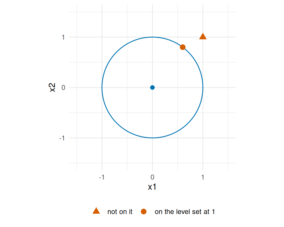
RemarkRemark 2 (Level sets in the plane)
DefDefinition 6 (Level curve)
Definition 6 (Level curve) Let \(f : \mathbb{R}^2 \to \mathbb{R}\) and let \(c\) be a real number. The level curve of \(f\) at \(c\) is the level set of \(f\) at \(c\) when it is a curve in the plane. It is the special case \(p = 2\) of a level set. A contour line is a level curve drawn on a plot of \(f\).
Example 6 (A level curve of \(x_1^2 + x_2^2\)) Let \(f(\mathord{\smash[b]{\underset{\raise.3ex\hbox{$\scriptstyle\sim$}}{x}}\vphantom{x}}) = x_1^2 + x_2^2\) for \(\mathord{\smash[b]{\underset{\raise.3ex\hbox{$\scriptstyle\sim$}}{x}}\vphantom{x}}= {(x_1, x_2)}^{\top}\). The level curve at \(4\) is the circle of radius \(2\) around \(\mathord{\smash[b]{\underset{\raise.3ex\hbox{$\scriptstyle\sim$}}{0}}\vphantom{0}}\).
LemTheorem 3 (Level sets of a linear function)
Theorem 3 (Level sets of a linear function) Let \({h\mathopen{}\left(\mathord{\smash[b]{\underset{\raise.3ex\hbox{$\scriptstyle\sim$}}{x}}\vphantom{x}}\right)\mathclose{}} = \mathord{\smash[b]{\underset{\raise.3ex\hbox{$\scriptstyle\sim$}}{\beta}}\vphantom{\beta}} \cdot \mathord{\smash[b]{\underset{\raise.3ex\hbox{$\scriptstyle\sim$}}{x}}\vphantom{x}} + \beta_{0}\) with \(\mathord{\smash[b]{\underset{\raise.3ex\hbox{$\scriptstyle\sim$}}{\beta}}\vphantom{\beta}}\neq \mathord{\smash[b]{\underset{\raise.3ex\hbox{$\scriptstyle\sim$}}{0}}\vphantom{0}}\). Every level set \({{{h}^{-1}\mathopen{}\left(\mathopen{}\left\{c\right\}\mathclose{}\right)\mathclose{}}}\) is a hyperplane with normal vector \(\mathord{\smash[b]{\underset{\raise.3ex\hbox{$\scriptstyle\sim$}}{\beta}}\vphantom{\beta}}\), parallel to the level set \({{{h}^{-1}\mathopen{}\left(\mathopen{}\left\{0\right\}\mathclose{}\right)\mathclose{}}}\). Its dimension is \(p - 1\): a point for \(p = 1\), a line for \(p = 2\), and a two-dimensional plane for \(p = 3\).
ProofProof
Proof. For any \(c\),
\[ \begin{aligned} {{{h}^{-1}\mathopen{}\left(\mathopen{}\left\{c\right\}\mathclose{}\right)\mathclose{}}} &= {\mathopen{}\left\{ \mathord{\smash[b]{\underset{\raise.3ex\hbox{$\scriptstyle\sim$}}{x}}\vphantom{x}}: \mathord{\smash[b]{\underset{\raise.3ex\hbox{$\scriptstyle\sim$}}{\beta}}\vphantom{\beta}} \cdot \mathord{\smash[b]{\underset{\raise.3ex\hbox{$\scriptstyle\sim$}}{x}}\vphantom{x}} + \beta_{0}= c \right\}\mathclose{}} \\ &= {\mathopen{}\left\{ \mathord{\smash[b]{\underset{\raise.3ex\hbox{$\scriptstyle\sim$}}{x}}\vphantom{x}}: \mathord{\smash[b]{\underset{\raise.3ex\hbox{$\scriptstyle\sim$}}{\beta}}\vphantom{\beta}} \cdot \mathord{\smash[b]{\underset{\raise.3ex\hbox{$\scriptstyle\sim$}}{x}}\vphantom{x}} + (\beta_{0}- c) = 0 \right\}\mathclose{}}. \end{aligned} \]
This is the hyperplane with normal vector \(\mathord{\smash[b]{\underset{\raise.3ex\hbox{$\scriptstyle\sim$}}{\beta}}\vphantom{\beta}}\) and offset \(\beta_{0}- c\). Changing \(c\) changes only the offset, so the level sets share the normal vector and are parallel. A hyperplane in \(\mathbb{R}^p\) has dimension \(p - 1\) by the hyperplane theorem, which gives the point, line and plane cases for \(p = 1, 2, 3\).
ExmExample 7 (Parallel level lines)
Example 7 (Parallel level lines) Let \({h\mathopen{}\left(\mathord{\smash[b]{\underset{\raise.3ex\hbox{$\scriptstyle\sim$}}{x}}\vphantom{x}}\right)\mathclose{}} = 2x_1 + x_2 + 1\), so \(\mathord{\smash[b]{\underset{\raise.3ex\hbox{$\scriptstyle\sim$}}{\beta}}\vphantom{\beta}}= {(2, 1)}^{\top}\) and \(\beta_{0}= 1\). The level set at \(c\) is the line \(x_2 = c - 1 - 2x_1\). For \(c = -1, 0, 1\) the lines are \(x_2 = -2 - 2x_1\), \(x_2 = -1 - 2x_1\) and \(x_2 = -2x_1\). They all have slope \(-2\) and differ only in the intercept, so they are parallel.
LemTheorem 4 (Stepping along the normal vector)
Theorem 4 (Stepping along the normal vector) Let \({h\mathopen{}\left(\mathord{\smash[b]{\underset{\raise.3ex\hbox{$\scriptstyle\sim$}}{x}}\vphantom{x}}\right)\mathclose{}} = \mathord{\smash[b]{\underset{\raise.3ex\hbox{$\scriptstyle\sim$}}{\beta}}\vphantom{\beta}} \cdot \mathord{\smash[b]{\underset{\raise.3ex\hbox{$\scriptstyle\sim$}}{x}}\vphantom{x}} + \beta_{0}\) with \(\mathord{\smash[b]{\underset{\raise.3ex\hbox{$\scriptstyle\sim$}}{\beta}}\vphantom{\beta}}\neq \mathord{\smash[b]{\underset{\raise.3ex\hbox{$\scriptstyle\sim$}}{0}}\vphantom{0}}\). For every \(\mathord{\smash[b]{\underset{\raise.3ex\hbox{$\scriptstyle\sim$}}{x}}\vphantom{x}}\in \mathbb{R}^p\) and \(t \in \mathbb{R}\),
\[ {h\mathopen{}\left(\mathord{\smash[b]{\underset{\raise.3ex\hbox{$\scriptstyle\sim$}}{x}}\vphantom{x}}+ t\mathord{\smash[b]{\underset{\raise.3ex\hbox{$\scriptstyle\sim$}}{\beta}}\vphantom{\beta}}\right)\mathclose{}} = {h\mathopen{}\left(\mathord{\smash[b]{\underset{\raise.3ex\hbox{$\scriptstyle\sim$}}{x}}\vphantom{x}}\right)\mathclose{}} + t{\mathopen{}\left\lVert\mathord{\smash[b]{\underset{\raise.3ex\hbox{$\scriptstyle\sim$}}{\beta}}\vphantom{\beta}}\right\rVert\mathclose{}}^2. \]
So a step along \(\mathord{\smash[b]{\underset{\raise.3ex\hbox{$\scriptstyle\sim$}}{\beta}}\vphantom{\beta}}\) with \(t > 0\) increases \(h\).
ProofProof
Proof. By linearity of the dot product,
\[ \begin{aligned} {h\mathopen{}\left(\mathord{\smash[b]{\underset{\raise.3ex\hbox{$\scriptstyle\sim$}}{x}}\vphantom{x}}+ t\mathord{\smash[b]{\underset{\raise.3ex\hbox{$\scriptstyle\sim$}}{\beta}}\vphantom{\beta}}\right)\mathclose{}} &= \mathord{\smash[b]{\underset{\raise.3ex\hbox{$\scriptstyle\sim$}}{\beta}}\vphantom{\beta}} \cdot \mathord{\smash[b]{\underset{\raise.3ex\hbox{$\scriptstyle\sim$}}{x}}\vphantom{x}}+ t\mathord{\smash[b]{\underset{\raise.3ex\hbox{$\scriptstyle\sim$}}{\beta}}\vphantom{\beta}} + \beta_{0}\\ &= \mathord{\smash[b]{\underset{\raise.3ex\hbox{$\scriptstyle\sim$}}{\beta}}\vphantom{\beta}} \cdot \mathord{\smash[b]{\underset{\raise.3ex\hbox{$\scriptstyle\sim$}}{x}}\vphantom{x}} + t\mathord{\smash[b]{\underset{\raise.3ex\hbox{$\scriptstyle\sim$}}{\beta}}\vphantom{\beta}} \cdot \mathord{\smash[b]{\underset{\raise.3ex\hbox{$\scriptstyle\sim$}}{\beta}}\vphantom{\beta}} + \beta_{0}\\ &= {h\mathopen{}\left(\mathord{\smash[b]{\underset{\raise.3ex\hbox{$\scriptstyle\sim$}}{x}}\vphantom{x}}\right)\mathclose{}} + t{\mathopen{}\left\lVert\mathord{\smash[b]{\underset{\raise.3ex\hbox{$\scriptstyle\sim$}}{\beta}}\vphantom{\beta}}\right\rVert\mathclose{}}^2. \end{aligned} \]
ExmExample 8 (A step along the normal vector)
Example 8 (A step along the normal vector) Let \({h\mathopen{}\left(\mathord{\smash[b]{\underset{\raise.3ex\hbox{$\scriptstyle\sim$}}{x}}\vphantom{x}}\right)\mathclose{}} = 2x_1 + x_2 + 1\), so \(\mathord{\smash[b]{\underset{\raise.3ex\hbox{$\scriptstyle\sim$}}{\beta}}\vphantom{\beta}}= {(2, 1)}^{\top}\) and \({\mathopen{}\left\lVert\mathord{\smash[b]{\underset{\raise.3ex\hbox{$\scriptstyle\sim$}}{\beta}}\vphantom{\beta}}\right\rVert\mathclose{}}^2 = 5\). At \(\mathord{\smash[b]{\underset{\raise.3ex\hbox{$\scriptstyle\sim$}}{x}}\vphantom{x}}= \mathord{\smash[b]{\underset{\raise.3ex\hbox{$\scriptstyle\sim$}}{0}}\vphantom{0}}\), \({h\mathopen{}\left(\mathord{\smash[b]{\underset{\raise.3ex\hbox{$\scriptstyle\sim$}}{0}}\vphantom{0}}\right)\mathclose{}} = 1\). A step of \(t = 1\) along \(\mathord{\smash[b]{\underset{\raise.3ex\hbox{$\scriptstyle\sim$}}{\beta}}\vphantom{\beta}}\) lands at \({(2, 1)}^{\top}\), where \({h\mathopen{}\left({(2, 1)}^{\top}\right)\mathclose{}} = 4 + 1 + 1 = 6 = 1 + 5\).
LemTheorem 5 (The normal vector is the steepest direction)
Theorem 5 (The normal vector is the steepest direction) Let \({h\mathopen{}\left(\mathord{\smash[b]{\underset{\raise.3ex\hbox{$\scriptstyle\sim$}}{x}}\vphantom{x}}\right)\mathclose{}} = \mathord{\smash[b]{\underset{\raise.3ex\hbox{$\scriptstyle\sim$}}{\beta}}\vphantom{\beta}} \cdot \mathord{\smash[b]{\underset{\raise.3ex\hbox{$\scriptstyle\sim$}}{x}}\vphantom{x}} + \beta_{0}\) with \(\mathord{\smash[b]{\underset{\raise.3ex\hbox{$\scriptstyle\sim$}}{\beta}}\vphantom{\beta}}\neq \mathord{\smash[b]{\underset{\raise.3ex\hbox{$\scriptstyle\sim$}}{0}}\vphantom{0}}\). Among unit vectors \(\mathord{\smash[b]{\underset{\raise.3ex\hbox{$\scriptstyle\sim$}}{u}}\vphantom{u}}\) (\(\mathopen{}\left\lVert\mathord{\smash[b]{\underset{\raise.3ex\hbox{$\scriptstyle\sim$}}{u}}\vphantom{u}}\right\rVert\mathclose{} = 1\)), the change \({h\mathopen{}\left(\mathord{\smash[b]{\underset{\raise.3ex\hbox{$\scriptstyle\sim$}}{x}}\vphantom{x}}+ t\mathord{\smash[b]{\underset{\raise.3ex\hbox{$\scriptstyle\sim$}}{u}}\vphantom{u}}\right)\mathclose{}} - {h\mathopen{}\left(\mathord{\smash[b]{\underset{\raise.3ex\hbox{$\scriptstyle\sim$}}{x}}\vphantom{x}}\right)\mathclose{}}\) with \(t > 0\) is largest for \(\mathord{\smash[b]{\underset{\raise.3ex\hbox{$\scriptstyle\sim$}}{u}}\vphantom{u}}= \mathord{\smash[b]{\underset{\raise.3ex\hbox{$\scriptstyle\sim$}}{\beta}}\vphantom{\beta}}/ \mathopen{}\left\lVert\mathord{\smash[b]{\underset{\raise.3ex\hbox{$\scriptstyle\sim$}}{\beta}}\vphantom{\beta}}\right\rVert\mathclose{}\).
ProofProof
Proof. For a unit vector \(\mathord{\smash[b]{\underset{\raise.3ex\hbox{$\scriptstyle\sim$}}{u}}\vphantom{u}}\),
\[ {h\mathopen{}\left(\mathord{\smash[b]{\underset{\raise.3ex\hbox{$\scriptstyle\sim$}}{x}}\vphantom{x}}+ t\mathord{\smash[b]{\underset{\raise.3ex\hbox{$\scriptstyle\sim$}}{u}}\vphantom{u}}\right)\mathclose{}} - {h\mathopen{}\left(\mathord{\smash[b]{\underset{\raise.3ex\hbox{$\scriptstyle\sim$}}{x}}\vphantom{x}}\right)\mathclose{}} = t\mathord{\smash[b]{\underset{\raise.3ex\hbox{$\scriptstyle\sim$}}{\beta}}\vphantom{\beta}} \cdot \mathord{\smash[b]{\underset{\raise.3ex\hbox{$\scriptstyle\sim$}}{u}}\vphantom{u}}. \]
Since \(t > 0\), maximizing this change is the same as maximizing \(\mathord{\smash[b]{\underset{\raise.3ex\hbox{$\scriptstyle\sim$}}{\beta}}\vphantom{\beta}} \cdot \mathord{\smash[b]{\underset{\raise.3ex\hbox{$\scriptstyle\sim$}}{u}}\vphantom{u}}\). By the Cauchy-Schwarz inequality, \(\mathord{\smash[b]{\underset{\raise.3ex\hbox{$\scriptstyle\sim$}}{\beta}}\vphantom{\beta}} \cdot \mathord{\smash[b]{\underset{\raise.3ex\hbox{$\scriptstyle\sim$}}{u}}\vphantom{u}} \le \mathopen{}\left\lVert\mathord{\smash[b]{\underset{\raise.3ex\hbox{$\scriptstyle\sim$}}{\beta}}\vphantom{\beta}}\right\rVert\mathclose{}\mathopen{}\left\lVert\mathord{\smash[b]{\underset{\raise.3ex\hbox{$\scriptstyle\sim$}}{u}}\vphantom{u}}\right\rVert\mathclose{} = \mathopen{}\left\lVert\mathord{\smash[b]{\underset{\raise.3ex\hbox{$\scriptstyle\sim$}}{\beta}}\vphantom{\beta}}\right\rVert\mathclose{}\). Equality holds exactly when \(\mathord{\smash[b]{\underset{\raise.3ex\hbox{$\scriptstyle\sim$}}{u}}\vphantom{u}}= \alpha\mathord{\smash[b]{\underset{\raise.3ex\hbox{$\scriptstyle\sim$}}{\beta}}\vphantom{\beta}}\) for some \(\alpha > 0\). The condition \(\mathopen{}\left\lVert\mathord{\smash[b]{\underset{\raise.3ex\hbox{$\scriptstyle\sim$}}{u}}\vphantom{u}}\right\rVert\mathclose{} = 1\) then forces \(\alpha\mathopen{}\left\lVert\mathord{\smash[b]{\underset{\raise.3ex\hbox{$\scriptstyle\sim$}}{\beta}}\vphantom{\beta}}\right\rVert\mathclose{} = 1\), so
\[ \mathord{\smash[b]{\underset{\raise.3ex\hbox{$\scriptstyle\sim$}}{u}}\vphantom{u}}= \mathord{\smash[b]{\underset{\raise.3ex\hbox{$\scriptstyle\sim$}}{\beta}}\vphantom{\beta}}/ \mathopen{}\left\lVert\mathord{\smash[b]{\underset{\raise.3ex\hbox{$\scriptstyle\sim$}}{\beta}}\vphantom{\beta}}\right\rVert\mathclose{}. \]
ExmExample 9 (Two unit steps compared)
Example 9 (Two unit steps compared) Let \({h\mathopen{}\left(\mathord{\smash[b]{\underset{\raise.3ex\hbox{$\scriptstyle\sim$}}{x}}\vphantom{x}}\right)\mathclose{}} = 2x_1 + x_2 + 1\), so \(\mathord{\smash[b]{\underset{\raise.3ex\hbox{$\scriptstyle\sim$}}{\beta}}\vphantom{\beta}}= {(2, 1)}^{\top}\) and \(\mathopen{}\left\lVert\mathord{\smash[b]{\underset{\raise.3ex\hbox{$\scriptstyle\sim$}}{\beta}}\vphantom{\beta}}\right\rVert\mathclose{} = \sqrt{5}\). A step of size \(1\) along the unit vector \(\mathord{\smash[b]{\underset{\raise.3ex\hbox{$\scriptstyle\sim$}}{\beta}}\vphantom{\beta}}/ \sqrt{5}\) raises \(h\) by \(\mathord{\smash[b]{\underset{\raise.3ex\hbox{$\scriptstyle\sim$}}{\beta}}\vphantom{\beta}} \cdot \mathord{\smash[b]{\underset{\raise.3ex\hbox{$\scriptstyle\sim$}}{\beta}}\vphantom{\beta}} / \sqrt{5} = \sqrt{5} \approx 2.24\). A step of size \(1\) along \({(1, 0)}^{\top}\) raises it by only \(\mathord{\smash[b]{\underset{\raise.3ex\hbox{$\scriptstyle\sim$}}{\beta}}\vphantom{\beta}} \cdot {(1, 0)}^{\top} = 2\).
Turn the blue arrow in Figure 3 and watch the rate: it is largest along the red arrow, zero along the black level curve (Definition 5), and most negative pointing straight back. Then look for a point where the red arrow shrinks to nothing.
ExrExercise 5 (Take a gradient by hand)
Exercise 5 (Take a gradient by hand) Let \(f : \mathbb{R}^2 \to \mathbb{R}\) be
\[f(\mathord{\smash[b]{\underset{\raise.3ex\hbox{$\scriptstyle\sim$}}{w}}\vphantom{w}}) = 3 w_1 w_2 + w_2^3 - 5 w_1\]
- Compute \(\partial f / \partial w_1\) (Definition 1), treating \(w_2\) as a constant.
- Compute \(\partial f / \partial w_2\), treating \(w_1\) as a constant.
- Assemble \(\nabla_{\mathord{\smash[b]{\underset{\raise.3ex\hbox{$\scriptstyle\sim$}}{w}}\vphantom{w}}} f\) and evaluate it at \(\mathord{\smash[b]{\underset{\raise.3ex\hbox{$\scriptstyle\sim$}}{w}}\vphantom{w}} = \begin{bmatrix} 2 & -1 \end{bmatrix}^{\top}\).
- Check the shape of your answer against Table 1.
DefDefinition 7 (Row-vector derivative)
Definition 7 (Row-vector derivative) If \(f(\mathord{\smash[b]{\underset{\raise.3ex\hbox{$\scriptstyle\sim$}}{\beta}}\vphantom{\beta}})\) is a scalar-valued function of a \(p \times 1\) vector \(\mathord{\smash[b]{\underset{\raise.3ex\hbox{$\scriptstyle\sim$}}{\beta}}\vphantom{\beta}}\), such as \(f(\mathord{\smash[b]{\underset{\raise.3ex\hbox{$\scriptstyle\sim$}}{\beta}}\vphantom{\beta}}) = \mathord{\smash[b]{\underset{\raise.3ex\hbox{$\scriptstyle\sim$}}{x}}\vphantom{x}} \cdot \mathord{\smash[b]{\underset{\raise.3ex\hbox{$\scriptstyle\sim$}}{\beta}}\vphantom{\beta}}\), then its row-vector derivative is the row vector of its partial derivatives (Definition 1):
\[ \frac{\partial f(\mathord{\smash[b]{\underset{\raise.3ex\hbox{$\scriptstyle\sim$}}{\beta}}\vphantom{\beta}})}{\partial {\mathord{\smash[b]{\underset{\raise.3ex\hbox{$\scriptstyle\sim$}}{\beta}}\vphantom{\beta}}}^{\top}} = \begin{bmatrix} \frac{\partial}{\partial \beta_{1}}f(\mathord{\smash[b]{\underset{\raise.3ex\hbox{$\scriptstyle\sim$}}{\beta}}\vphantom{\beta}}) & \frac{\partial}{\partial \beta_{2}}f(\mathord{\smash[b]{\underset{\raise.3ex\hbox{$\scriptstyle\sim$}}{\beta}}\vphantom{\beta}}) & \cdots & \frac{\partial}{\partial \beta_{p}}f(\mathord{\smash[b]{\underset{\raise.3ex\hbox{$\scriptstyle\sim$}}{\beta}}\vphantom{\beta}}) \end{bmatrix} \tag{2}\]
When the derivative of a scalar-valued function is written as a row vector, it is also called the total derivative [8] of \(f\).
RemarkRemark 3 (Other notation for the row-vector derivative)
Remark 3 (Other notation for the row-vector derivative). Some sources write the same row vector as \(\frac{\partial}{\partial {\mathord{\smash[b]{\underset{\raise.3ex\hbox{$\scriptstyle\sim$}}{\beta}}\vphantom{\beta}}}^{\top}} f(\mathord{\smash[b]{\underset{\raise.3ex\hbox{$\scriptstyle\sim$}}{\beta}}\vphantom{\beta}})\), with the operator on the left, read as each operator \(\frac{\partial}{\partial \beta_{i}}\) applied to \(f\) rather than as a matrix product (see Remark 4).
RemarkRemark 4 (Which side the operator goes on)
Remark 4 (Which side the operator goes on). Read \(\frac{\partial}{\partial \mathord{\smash[b]{\underset{\raise.3ex\hbox{$\scriptstyle\sim$}}{\beta}}\vphantom{\beta}}}\) as a \(p \times 1\) column vector of operators with entries \(\frac{\partial}{\partial \beta_{1}}, \ldots, \frac{\partial}{\partial \beta_{p}}\), and \(\frac{\partial}{\partial {\mathord{\smash[b]{\underset{\raise.3ex\hbox{$\scriptstyle\sim$}}{\beta}}\vphantom{\beta}}}^{\top}}\) as the \(1 \times p\) row vector of operators with the same entries. Writing either one next to \(f\) can be read in two ways:
- As a matrix product, with \(f\) a \(1 \times 1\) matrix, under the shape rule of matrix multiplication. The column-vector operator works on the left: \(\frac{\partial}{\partial \mathord{\smash[b]{\underset{\raise.3ex\hbox{$\scriptstyle\sim$}}{\beta}}\vphantom{\beta}}} f\) is \((p \times 1)(1 \times 1)\), a \(p \times 1\) column vector (Definition 2). The row-vector operator does not: \(\frac{\partial}{\partial {\mathord{\smash[b]{\underset{\raise.3ex\hbox{$\scriptstyle\sim$}}{\beta}}\vphantom{\beta}}}^{\top}} f\) is \((1 \times p)(1 \times 1)\), whose inner dimensions \(p\) and \(1\) do not match when \(p > 1\). For the shape rule to give the \(1 \times p\) row vector, the operator would have to go on the right of \(f\), as in \((1 \times 1)(1 \times p)\), which changes its meaning (see below).
- As a scalar multiple, with \(f\) a scalar, the way \(c \mathord{\smash[b]{\underset{\raise.3ex\hbox{$\scriptstyle\sim$}}{x}}\vphantom{x}}\) is read in scalar multiplication, which has no shape rule: each entry of the operator vector is applied to \(f\). Then both \(\frac{\partial}{\partial \mathord{\smash[b]{\underset{\raise.3ex\hbox{$\scriptstyle\sim$}}{\beta}}\vphantom{\beta}}} f\) and \(\frac{\partial}{\partial {\mathord{\smash[b]{\underset{\raise.3ex\hbox{$\scriptstyle\sim$}}{\beta}}\vphantom{\beta}}}^{\top}} f\) work with the operator on the left.
The fraction \(\frac{\partial f}{\partial {\mathord{\smash[b]{\underset{\raise.3ex\hbox{$\scriptstyle\sim$}}{\beta}}\vphantom{\beta}}}^{\top}}\) of Equation 2 means the same thing under both readings: the transpose in the denominator says the result is a row vector, without making the derivative a product.
Treating the operators as vectors is sound for checking shapes, but “multiplying” an operator by a function means applying the operator to it, so two rules of ordinary matrix algebra do not carry over: scalars commute with matrices, and products can be regrouped.
- Scalars do not commute with operators. \(\frac{\partial}{\partial \beta_{i}} f\) is a function, but \(f \frac{\partial}{\partial \beta_{i}}\) is still an unapplied operator, waiting for something to act on. So, unlike \(c \mathord{\smash[b]{\underset{\raise.3ex\hbox{$\scriptstyle\sim$}}{x}}\vphantom{x}}= \mathord{\smash[b]{\underset{\raise.3ex\hbox{$\scriptstyle\sim$}}{x}}\vphantom{x}}c\), the operator cannot move to the other side of \(f\) without changing the meaning. Putting the row-vector operator on the right of \(f\) gives the row-vector derivative only under the convention that it acts on the factor to its left.
- Products cannot be regrouped. An operator acts on the whole product to its right, so by the product rule, \(\frac{\partial}{\partial \beta_{i}} (f g) \ne \mathopen{}\left(\frac{\partial}{\partial \beta_{i}} f\right)\mathclose{} g\) in general. For example, with \(f(\mathord{\smash[b]{\underset{\raise.3ex\hbox{$\scriptstyle\sim$}}{\beta}}\vphantom{\beta}}) = \beta_{1}\), \(\frac{\partial}{\partial \beta_{1}} (f f) = 2 \beta_{1}\) but \(\mathopen{}\left(\frac{\partial}{\partial \beta_{1}} f\right)\mathclose{} f = \beta_{1}\).
LemTheorem 6 (Row and column derivatives are transposes)
Theorem 6 (Row and column derivatives are transposes) \[\frac{\partial f(\mathord{\smash[b]{\underset{\raise.3ex\hbox{$\scriptstyle\sim$}}{\beta}}\vphantom{\beta}})}{\partial {\mathord{\smash[b]{\underset{\raise.3ex\hbox{$\scriptstyle\sim$}}{\beta}}\vphantom{\beta}}}^{\top}} = {\mathopen{}\left(\frac{\partial f(\mathord{\smash[b]{\underset{\raise.3ex\hbox{$\scriptstyle\sim$}}{\beta}}\vphantom{\beta}})}{\partial \mathord{\smash[b]{\underset{\raise.3ex\hbox{$\scriptstyle\sim$}}{\beta}}\vphantom{\beta}}}\right)\mathclose{}}^{\top} \tag{3}\]
\[\frac{\partial f(\mathord{\smash[b]{\underset{\raise.3ex\hbox{$\scriptstyle\sim$}}{\beta}}\vphantom{\beta}})}{\partial \mathord{\smash[b]{\underset{\raise.3ex\hbox{$\scriptstyle\sim$}}{\beta}}\vphantom{\beta}}} = {\mathopen{}\left(\frac{\partial f(\mathord{\smash[b]{\underset{\raise.3ex\hbox{$\scriptstyle\sim$}}{\beta}}\vphantom{\beta}})}{\partial {\mathord{\smash[b]{\underset{\raise.3ex\hbox{$\scriptstyle\sim$}}{\beta}}\vphantom{\beta}}}^{\top}}\right)\mathclose{}}^{\top} \tag{4}\]
ProofProof
Proof. By Definition 2 and Definition 7, entry \(j\) of both \(\frac{\partial f(\mathord{\smash[b]{\underset{\raise.3ex\hbox{$\scriptstyle\sim$}}{\beta}}\vphantom{\beta}})}{\partial \mathord{\smash[b]{\underset{\raise.3ex\hbox{$\scriptstyle\sim$}}{\beta}}\vphantom{\beta}}}\) and \(\frac{\partial f(\mathord{\smash[b]{\underset{\raise.3ex\hbox{$\scriptstyle\sim$}}{\beta}}\vphantom{\beta}})}{\partial {\mathord{\smash[b]{\underset{\raise.3ex\hbox{$\scriptstyle\sim$}}{\beta}}\vphantom{\beta}}}^{\top}}\) is \(\frac{\partial}{\partial \beta_{j}} f(\mathord{\smash[b]{\underset{\raise.3ex\hbox{$\scriptstyle\sim$}}{\beta}}\vphantom{\beta}})\); the first is a \(p \times 1\) column vector and the second a \(1 \times p\) row vector with the same entries in the same order, so each is the transpose of the other.
ExmExample 10 (Row and column derivatives of a linear function)
Example 10 (Row and column derivatives of a linear function) For \(f(\mathord{\smash[b]{\underset{\raise.3ex\hbox{$\scriptstyle\sim$}}{\beta}}\vphantom{\beta}}) = 3\beta_{1} + 5\beta_{2}\):
\[ \frac{\partial f(\mathord{\smash[b]{\underset{\raise.3ex\hbox{$\scriptstyle\sim$}}{\beta}}\vphantom{\beta}})}{\partial \mathord{\smash[b]{\underset{\raise.3ex\hbox{$\scriptstyle\sim$}}{\beta}}\vphantom{\beta}}} = \begin{bmatrix}3 \\ 5\end{bmatrix}, \qquad \frac{\partial f(\mathord{\smash[b]{\underset{\raise.3ex\hbox{$\scriptstyle\sim$}}{\beta}}\vphantom{\beta}})}{\partial {\mathord{\smash[b]{\underset{\raise.3ex\hbox{$\scriptstyle\sim$}}{\beta}}\vphantom{\beta}}}^{\top}} = \begin{bmatrix}3 & 5\end{bmatrix}, \]
and each is the transpose of the other.
DefDefinition 8 (Derivative of a vector-valued function)
Definition 8 (Derivative of a vector-valued function) If
\[ \begin{aligned} \mathord{\smash[b]{\underset{\raise.3ex\hbox{$\scriptstyle\sim$}}{y}}\vphantom{y}}&= \mathord{\smash[b]{\underset{\raise.3ex\hbox{$\scriptstyle\sim$}}{y}}\vphantom{y}}(\mathord{\smash[b]{\underset{\raise.3ex\hbox{$\scriptstyle\sim$}}{\beta}}\vphantom{\beta}}) \\ &= {(y_1, \ldots, y_q)}^{\top} \end{aligned} \]
is a \(q \times 1\) vector-valued function of the \(p \times 1\) vector \(\mathord{\smash[b]{\underset{\raise.3ex\hbox{$\scriptstyle\sim$}}{\beta}}\vphantom{\beta}}\), its derivative with respect to \(\mathord{\smash[b]{\underset{\raise.3ex\hbox{$\scriptstyle\sim$}}{\beta}}\vphantom{\beta}}\) is the \(p \times q\) matrix whose \((i, j)\) entry is
\[ \mathopen{}\left[\frac{\partial}{\partial \mathord{\smash[b]{\underset{\raise.3ex\hbox{$\scriptstyle\sim$}}{\beta}}\vphantom{\beta}}} {\mathord{\smash[b]{\underset{\raise.3ex\hbox{$\scriptstyle\sim$}}{y}}\vphantom{y}}}^{\top}\right]\mathclose{}_{ij} \stackrel{\text{def}}{=}\frac{\partial}{\partial \beta_{i}} y_j, \qquad i = 1, \ldots, p, \quad j = 1, \ldots, q. \]
Both \(\frac{\partial}{\partial \mathord{\smash[b]{\underset{\raise.3ex\hbox{$\scriptstyle\sim$}}{\beta}}\vphantom{\beta}}} \mathord{\smash[b]{\underset{\raise.3ex\hbox{$\scriptstyle\sim$}}{y}}\vphantom{y}}\) and \(\frac{\partial}{\partial \mathord{\smash[b]{\underset{\raise.3ex\hbox{$\scriptstyle\sim$}}{\beta}}\vphantom{\beta}}} {\mathord{\smash[b]{\underset{\raise.3ex\hbox{$\scriptstyle\sim$}}{y}}\vphantom{y}}}^{\top}\) denote this \(p \times q\) matrix.
DefDefinition 9 (Denominator layout)
Definition 9 (Denominator layout) Writing derivatives as in Definition 8 is the denominator layout [9], which these notes use throughout: rows index the entries of \(\mathord{\smash[b]{\underset{\raise.3ex\hbox{$\scriptstyle\sim$}}{\beta}}\vphantom{\beta}}\) (the denominator) and columns index the entries of \(\mathord{\smash[b]{\underset{\raise.3ex\hbox{$\scriptstyle\sim$}}{y}}\vphantom{y}}\) (the numerator), so column \(j\) is the vector derivative \(\frac{\partial}{\partial \mathord{\smash[b]{\underset{\raise.3ex\hbox{$\scriptstyle\sim$}}{\beta}}\vphantom{\beta}}} y_j\) (Definition 2).
Example 11 (Differentiating a \(3 \times 1\) function of a \(2 \times 1\) vector) Let \(\mathord{\smash[b]{\underset{\raise.3ex\hbox{$\scriptstyle\sim$}}{\beta}}\vphantom{\beta}}= {(\beta_{1}, \beta_{2})}^{\top}\) (\(p = 2\)) and \(\mathord{\smash[b]{\underset{\raise.3ex\hbox{$\scriptstyle\sim$}}{y}}\vphantom{y}}(\mathord{\smash[b]{\underset{\raise.3ex\hbox{$\scriptstyle\sim$}}{\beta}}\vphantom{\beta}}) = {(\beta_{1}^2,\ \beta_{1}\beta_{2},\ 3\beta_{2})}^{\top}\) (\(q = 3\)). Then
\[ \begin{aligned} \underbrace{\frac{\partial}{\partial \mathord{\smash[b]{\underset{\raise.3ex\hbox{$\scriptstyle\sim$}}{\beta}}\vphantom{\beta}}} {\mathord{\smash[b]{\underset{\raise.3ex\hbox{$\scriptstyle\sim$}}{y}}\vphantom{y}}}^{\top}}_{2 \times 3} &= \begin{bmatrix} \frac{\partial}{\partial \beta_{1}} \beta_{1}^2 & \frac{\partial}{\partial \beta_{1}} \beta_{1}\beta_{2} & \frac{\partial}{\partial \beta_{1}} 3\beta_{2} \\ \frac{\partial}{\partial \beta_{2}} \beta_{1}^2 & \frac{\partial}{\partial \beta_{2}} \beta_{1}\beta_{2} & \frac{\partial}{\partial \beta_{2}} 3\beta_{2} \end{bmatrix} \\ &= \begin{bmatrix} 2\beta_{1} & \beta_{2} & 0 \\ 0 & \beta_{1} & 3 \end{bmatrix} \end{aligned} \]
DefDefinition 10 (Jacobian matrix)
Definition 10 (Jacobian matrix) Let
\[ \begin{aligned} \mathord{\smash[b]{\underset{\raise.3ex\hbox{$\scriptstyle\sim$}}{y}}\vphantom{y}}&= \mathord{\smash[b]{\underset{\raise.3ex\hbox{$\scriptstyle\sim$}}{y}}\vphantom{y}}(\mathord{\smash[b]{\underset{\raise.3ex\hbox{$\scriptstyle\sim$}}{\beta}}\vphantom{\beta}}) \\ &= {(y_1, \ldots, y_q)}^{\top} \end{aligned} \]
be a \(q \times 1\) vector-valued function of the \(p \times 1\) vector \(\mathord{\smash[b]{\underset{\raise.3ex\hbox{$\scriptstyle\sim$}}{\beta}}\vphantom{\beta}}\). The Jacobian matrix [10] of \(\mathord{\smash[b]{\underset{\raise.3ex\hbox{$\scriptstyle\sim$}}{y}}\vphantom{y}}\) is the \(q \times p\) matrix whose \((j, i)\) entry is \(\frac{\partial}{\partial \beta_{i}} y_j\), for \(j = 1, \ldots, q\) and \(i = 1, \ldots, p\). It is the transpose of the derivative \(\frac{\partial}{\partial \mathord{\smash[b]{\underset{\raise.3ex\hbox{$\scriptstyle\sim$}}{\beta}}\vphantom{\beta}}} {\mathord{\smash[b]{\underset{\raise.3ex\hbox{$\scriptstyle\sim$}}{y}}\vphantom{y}}}^{\top}\) of Definition 8.
DefDefinition 11 (Numerator layout)
Definition 11 (Numerator layout) Writing derivatives as in Definition 10, with rows indexing the entries of \(\mathord{\smash[b]{\underset{\raise.3ex\hbox{$\scriptstyle\sim$}}{y}}\vphantom{y}}\) (the numerator) and columns indexing the entries of \(\mathord{\smash[b]{\underset{\raise.3ex\hbox{$\scriptstyle\sim$}}{\beta}}\vphantom{\beta}}\) (the denominator), is the numerator layout [9].
Example 12 (The Jacobian matrix of a \(3 \times 1\) function of a \(2 \times 1\) vector) For \(\mathord{\smash[b]{\underset{\raise.3ex\hbox{$\scriptstyle\sim$}}{y}}\vphantom{y}}(\mathord{\smash[b]{\underset{\raise.3ex\hbox{$\scriptstyle\sim$}}{\beta}}\vphantom{\beta}}) = {(\beta_{1}^2,\ \beta_{1}\beta_{2},\ 3\beta_{2})}^{\top}\) of Example 11, the Jacobian matrix is the \(3 \times 2\) matrix
\[ \begin{bmatrix} \frac{\partial}{\partial \beta_{1}} \beta_{1}^2 & \frac{\partial}{\partial \beta_{2}} \beta_{1}^2 \\ \frac{\partial}{\partial \beta_{1}} \beta_{1}\beta_{2} & \frac{\partial}{\partial \beta_{2}} \beta_{1}\beta_{2} \\ \frac{\partial}{\partial \beta_{1}} 3\beta_{2} & \frac{\partial}{\partial \beta_{2}} 3\beta_{2} \end{bmatrix} = \begin{bmatrix} 2\beta_{1} & 0 \\ \beta_{2} & \beta_{1} \\ 0 & 3 \end{bmatrix}, \]
the transpose of the \(2 \times 3\) matrix found there.
RemarkRemark 5 (Numerator layout)
Remark 5 (Numerator layout). Some sources use the numerator layout (Definition 11) throughout, so that their derivative of a vector-valued function is the Jacobian matrix, the transpose of the derivative used in these notes. In numerator layout, the derivative of a scalar-valued function is a row vector: the row-vector derivative (Definition 7). Check a source’s layout before combining its formulas with these.
DefDefinition 12 (Constant)
Definition 12 (Constant) A \(q \times 1\) vector \(\mathord{\smash[b]{\underset{\raise.3ex\hbox{$\scriptstyle\sim$}}{x}}\vphantom{x}}\) is constant with respect to the \(p \times 1\) vector \(\mathord{\smash[b]{\underset{\raise.3ex\hbox{$\scriptstyle\sim$}}{\beta}}\vphantom{\beta}}\) if its derivative (Definition 8) is zero:
\[ \underbrace{\frac{\partial}{\partial \mathord{\smash[b]{\underset{\raise.3ex\hbox{$\scriptstyle\sim$}}{\beta}}\vphantom{\beta}}} {\mathord{\smash[b]{\underset{\raise.3ex\hbox{$\scriptstyle\sim$}}{x}}\vphantom{x}}}^{\top}}_{p \times q} = \underbrace{\mathbf{0}}_{p \times q} \]
ExmExample 13 (A constant vector)
Example 13 (A constant vector) Let \(\mathord{\smash[b]{\underset{\raise.3ex\hbox{$\scriptstyle\sim$}}{\beta}}\vphantom{\beta}}= {(\beta_{1}, \beta_{2})}^{\top}\) and \(\mathord{\smash[b]{\underset{\raise.3ex\hbox{$\scriptstyle\sim$}}{x}}\vphantom{x}}= {(3, 5)}^{\top}\), so \(x_1 = 3\) and \(x_2 = 5\) do not depend on \(\mathord{\smash[b]{\underset{\raise.3ex\hbox{$\scriptstyle\sim$}}{\beta}}\vphantom{\beta}}\). Expanding \(\frac{\partial}{\partial \mathord{\smash[b]{\underset{\raise.3ex\hbox{$\scriptstyle\sim$}}{\beta}}\vphantom{\beta}}} {\mathord{\smash[b]{\underset{\raise.3ex\hbox{$\scriptstyle\sim$}}{x}}\vphantom{x}}}^{\top}\) into its matrix of scalar partial derivatives (Definition 8) and evaluating each entry:
\[ \begin{aligned} \underbrace{\frac{\partial}{\partial \mathord{\smash[b]{\underset{\raise.3ex\hbox{$\scriptstyle\sim$}}{\beta}}\vphantom{\beta}}} {\mathord{\smash[b]{\underset{\raise.3ex\hbox{$\scriptstyle\sim$}}{x}}\vphantom{x}}}^{\top}}_{2 \times 2} &= \frac{\partial}{\partial \mathord{\smash[b]{\underset{\raise.3ex\hbox{$\scriptstyle\sim$}}{\beta}}\vphantom{\beta}}} \begin{bmatrix}x_1 & x_2\end{bmatrix} \\ &= \begin{bmatrix} \frac{\partial}{\partial \beta_{1}} x_1 & \frac{\partial}{\partial \beta_{1}} x_2 \\ \frac{\partial}{\partial \beta_{2}} x_1 & \frac{\partial}{\partial \beta_{2}} x_2 \end{bmatrix} \\ &= \begin{bmatrix} \frac{\partial}{\partial \beta_{1}} 3 & \frac{\partial}{\partial \beta_{1}} 5 \\ \frac{\partial}{\partial \beta_{2}} 3 & \frac{\partial}{\partial \beta_{2}} 5 \end{bmatrix} \\ &= \begin{bmatrix} 0 & 0 \\ 0 & 0 \end{bmatrix} \\ &= \underbrace{\mathbf{0}}_{2 \times 2} \end{aligned} \]
Every entry is the derivative of a constant, so \(\frac{\partial}{\partial \mathord{\smash[b]{\underset{\raise.3ex\hbox{$\scriptstyle\sim$}}{\beta}}\vphantom{\beta}}} {\mathord{\smash[b]{\underset{\raise.3ex\hbox{$\scriptstyle\sim$}}{x}}\vphantom{x}}}^{\top} = \underbrace{\mathbf{0}}_{2 \times 2}\) and \(\mathord{\smash[b]{\underset{\raise.3ex\hbox{$\scriptstyle\sim$}}{x}}\vphantom{x}}\) is constant with respect to \(\mathord{\smash[b]{\underset{\raise.3ex\hbox{$\scriptstyle\sim$}}{\beta}}\vphantom{\beta}}\) (Definition 12).
ExmExample 14 (A vector that is not constant)
Example 14 (A vector that is not constant) With the same \(\mathord{\smash[b]{\underset{\raise.3ex\hbox{$\scriptstyle\sim$}}{\beta}}\vphantom{\beta}}\), let \(\mathord{\smash[b]{\underset{\raise.3ex\hbox{$\scriptstyle\sim$}}{x}}\vphantom{x}}= {(\beta_{1}, 3)}^{\top}\). Then
\[ \begin{aligned} \underbrace{\frac{\partial}{\partial \mathord{\smash[b]{\underset{\raise.3ex\hbox{$\scriptstyle\sim$}}{\beta}}\vphantom{\beta}}} {\mathord{\smash[b]{\underset{\raise.3ex\hbox{$\scriptstyle\sim$}}{x}}\vphantom{x}}}^{\top}}_{2 \times 2} &= \begin{bmatrix} \frac{\partial}{\partial \beta_{1}} \beta_{1} & \frac{\partial}{\partial \beta_{1}} 3 \\ \frac{\partial}{\partial \beta_{2}} \beta_{1} & \frac{\partial}{\partial \beta_{2}} 3 \end{bmatrix} \\ &= \begin{bmatrix} 1 & 0 \\ 0 & 0 \end{bmatrix}, \end{aligned} \]
which is not \(\underbrace{\mathbf{0}}_{2 \times 2}\), so this \(\mathord{\smash[b]{\underset{\raise.3ex\hbox{$\scriptstyle\sim$}}{x}}\vphantom{x}}\) is not constant with respect to \(\mathord{\smash[b]{\underset{\raise.3ex\hbox{$\scriptstyle\sim$}}{\beta}}\vphantom{\beta}}\): its first entry changes when \(\beta_{1}\) does.
ExrExercise 6 (Partial derivative with respect to an unreferenced variable)
Exercise 6 (Partial derivative with respect to an unreferenced variable) Adapted from Miller [3], Question 1.1.46.
Find \(\frac{\partial f}{\partial x}\) and \(\frac{\partial f}{\partial y}\) for
\[f(x, y, t) = 5t^4 - 4t^5 \cos(t\sin t)\]
LemTheorem 7 (Derivative of a dot product)
Theorem 7 (Derivative of a dot product) If \(\mathord{\smash[b]{\underset{\raise.3ex\hbox{$\scriptstyle\sim$}}{x}}\vphantom{x}}\) is constant with respect to \(\mathord{\smash[b]{\underset{\raise.3ex\hbox{$\scriptstyle\sim$}}{\beta}}\vphantom{\beta}}\), then:
\[ \begin{aligned} \underbrace{\frac{\partial}{\partial \mathord{\smash[b]{\underset{\raise.3ex\hbox{$\scriptstyle\sim$}}{\beta}}\vphantom{\beta}}} (\mathord{\smash[b]{\underset{\raise.3ex\hbox{$\scriptstyle\sim$}}{x}}\vphantom{x}}\cdot \mathord{\smash[b]{\underset{\raise.3ex\hbox{$\scriptstyle\sim$}}{\beta}}\vphantom{\beta}})}_{p \times 1} &= \underbrace{\frac{\partial}{\partial \mathord{\smash[b]{\underset{\raise.3ex\hbox{$\scriptstyle\sim$}}{\beta}}\vphantom{\beta}}} (\mathord{\smash[b]{\underset{\raise.3ex\hbox{$\scriptstyle\sim$}}{\beta}}\vphantom{\beta}}\cdot \mathord{\smash[b]{\underset{\raise.3ex\hbox{$\scriptstyle\sim$}}{x}}\vphantom{x}})}_{p \times 1} \\ &= \underbrace{\mathord{\smash[b]{\underset{\raise.3ex\hbox{$\scriptstyle\sim$}}{x}}\vphantom{x}}}_{p \times 1} \end{aligned} \]
ProofProof
Proof. \[ \begin{aligned} \frac{\partial}{\partial \mathord{\smash[b]{\underset{\raise.3ex\hbox{$\scriptstyle\sim$}}{\beta}}\vphantom{\beta}}} (\mathord{\smash[b]{\underset{\raise.3ex\hbox{$\scriptstyle\sim$}}{x}}\vphantom{x}}\cdot \mathord{\smash[b]{\underset{\raise.3ex\hbox{$\scriptstyle\sim$}}{\beta}}\vphantom{\beta}}) &= \begin{bmatrix} \frac{\partial}{\partial \beta_{1}}(x_1\beta_{1}+x_2\beta_{2} +...+x_p \beta_{p} ) \\ \frac{\partial}{\partial \beta_{2}}(x_1\beta_{1}+x_2\beta_{2} +...+x_p \beta_{p} ) \\ \vdots \\ \frac{\partial}{\partial \beta_{p}}(x_1\beta_{1}+x_2\beta_{2} +...+x_p \beta_{p} ) \end{bmatrix} \\ &= \begin{bmatrix} x_{1} \\ x_{2} \\ \vdots \\ x_{p} \end{bmatrix} \\ &= \mathord{\smash[b]{\underset{\raise.3ex\hbox{$\scriptstyle\sim$}}{x}}\vphantom{x}} \end{aligned} \]
ExmExample 15 (Derivative of a dot product)
Example 15 (Derivative of a dot product) Let \(\mathord{\smash[b]{\underset{\raise.3ex\hbox{$\scriptstyle\sim$}}{x}}\vphantom{x}}= {(3, 5)}^{\top}\) (constant with respect to \(\mathord{\smash[b]{\underset{\raise.3ex\hbox{$\scriptstyle\sim$}}{\beta}}\vphantom{\beta}}\); see Example 13) and \(\mathord{\smash[b]{\underset{\raise.3ex\hbox{$\scriptstyle\sim$}}{\beta}}\vphantom{\beta}}= {(\beta_{1}, \beta_{2})}^{\top}\). Then \(\mathord{\smash[b]{\underset{\raise.3ex\hbox{$\scriptstyle\sim$}}{x}}\vphantom{x}}\cdot \mathord{\smash[b]{\underset{\raise.3ex\hbox{$\scriptstyle\sim$}}{\beta}}\vphantom{\beta}}= 3\beta_{1} + 5\beta_{2}\), and by Theorem 7:
\[ \begin{aligned} \underbrace{\frac{\partial}{\partial \mathord{\smash[b]{\underset{\raise.3ex\hbox{$\scriptstyle\sim$}}{\beta}}\vphantom{\beta}}}(\mathord{\smash[b]{\underset{\raise.3ex\hbox{$\scriptstyle\sim$}}{x}}\vphantom{x}}\cdot \mathord{\smash[b]{\underset{\raise.3ex\hbox{$\scriptstyle\sim$}}{\beta}}\vphantom{\beta}})}_{2 \times 1} &= \underbrace{\mathord{\smash[b]{\underset{\raise.3ex\hbox{$\scriptstyle\sim$}}{x}}\vphantom{x}}}_{2 \times 1} \\ &= \begin{pmatrix} 3 \\ 5 \end{pmatrix} \end{aligned} \]
Verifying entry-wise:
\[ \begin{aligned} \frac{\partial}{\partial \mathord{\smash[b]{\underset{\raise.3ex\hbox{$\scriptstyle\sim$}}{\beta}}\vphantom{\beta}}}(3\beta_{1} + 5\beta_{2}) &= \begin{pmatrix} \frac{\partial}{\partial \beta_{1}}(3\beta_{1} + 5\beta_{2}) \\ \frac{\partial}{\partial \beta_{2}}(3\beta_{1} + 5\beta_{2}) \end{pmatrix} \\ &= \begin{pmatrix} 3 \\ 5 \end{pmatrix} \end{aligned} \]
Both methods agree.
LemTheorem 8 (Product rule for dot-products)
Theorem 8 (Product rule for dot-products) If \(\mathord{\smash[b]{\underset{\raise.3ex\hbox{$\scriptstyle\sim$}}{a}}\vphantom{a}} = \mathord{\smash[b]{\underset{\raise.3ex\hbox{$\scriptstyle\sim$}}{a}}\vphantom{a}}(\mathord{\smash[b]{\underset{\raise.3ex\hbox{$\scriptstyle\sim$}}{x}}\vphantom{x}})\) and \(\mathord{\smash[b]{\underset{\raise.3ex\hbox{$\scriptstyle\sim$}}{b}}\vphantom{b}} = \mathord{\smash[b]{\underset{\raise.3ex\hbox{$\scriptstyle\sim$}}{b}}\vphantom{b}}(\mathord{\smash[b]{\underset{\raise.3ex\hbox{$\scriptstyle\sim$}}{x}}\vphantom{x}})\) are differentiable \(p \times 1\) vector functions of \(\mathord{\smash[b]{\underset{\raise.3ex\hbox{$\scriptstyle\sim$}}{x}}\vphantom{x}}\), then:
\[ \begin{aligned} \frac{\partial}{\partial \underbrace{\mathord{\smash[b]{\underset{\raise.3ex\hbox{$\scriptstyle\sim$}}{x}}\vphantom{x}}}_{p \times 1}} \underbrace{\mathord{\smash[b]{\underset{\raise.3ex\hbox{$\scriptstyle\sim$}}{a}}\vphantom{a}}}_{p \times 1} \cdot \underbrace{\mathord{\smash[b]{\underset{\raise.3ex\hbox{$\scriptstyle\sim$}}{b}}\vphantom{b}}}_{p \times 1} &= \mathopen{}\left( \frac{\partial}{\partial \underbrace{\mathord{\smash[b]{\underset{\raise.3ex\hbox{$\scriptstyle\sim$}}{x}}\vphantom{x}}}_{p \times 1}} \underbrace{{\mathord{\smash[b]{\underset{\raise.3ex\hbox{$\scriptstyle\sim$}}{a}}\vphantom{a}}}^{\top}}_{1 \times p} \right)\mathclose{} \underbrace{\mathord{\smash[b]{\underset{\raise.3ex\hbox{$\scriptstyle\sim$}}{b}}\vphantom{b}}}_{p \times 1} + \mathopen{}\left( \frac{\partial}{\partial \underbrace{\mathord{\smash[b]{\underset{\raise.3ex\hbox{$\scriptstyle\sim$}}{x}}\vphantom{x}}}_{p \times 1}} \underbrace{{\mathord{\smash[b]{\underset{\raise.3ex\hbox{$\scriptstyle\sim$}}{b}}\vphantom{b}}}^{\top}}_{1 \times p} \right)\mathclose{} \underbrace{\mathord{\smash[b]{\underset{\raise.3ex\hbox{$\scriptstyle\sim$}}{a}}\vphantom{a}}}_{p \times 1} \end{aligned} \]
ProofProof
Proof. Entry-wise, for \(i = 1, \ldots, p\):
\[ \begin{aligned} \mathopen{}\left[\frac{\partial}{\partial \mathord{\smash[b]{\underset{\raise.3ex\hbox{$\scriptstyle\sim$}}{x}}\vphantom{x}}} (\mathord{\smash[b]{\underset{\raise.3ex\hbox{$\scriptstyle\sim$}}{a}}\vphantom{a}} \cdot \mathord{\smash[b]{\underset{\raise.3ex\hbox{$\scriptstyle\sim$}}{b}}\vphantom{b}})\right]\mathclose{}_i &= \frac{\partial}{\partial x_i} \sum_{k=1}^{p} a_k b_k \\ &= \sum_{k=1}^{p} \mathopen{}\left(b_k \frac{\partial}{\partial x_i} a_k + a_k \frac{\partial}{\partial x_i} b_k\right)\mathclose{} \\ &= \mathopen{}\left[\mathopen{}\left(\frac{\partial}{\partial \mathord{\smash[b]{\underset{\raise.3ex\hbox{$\scriptstyle\sim$}}{x}}\vphantom{x}}} {\mathord{\smash[b]{\underset{\raise.3ex\hbox{$\scriptstyle\sim$}}{a}}\vphantom{a}}}^{\top}\right)\mathclose{}\mathord{\smash[b]{\underset{\raise.3ex\hbox{$\scriptstyle\sim$}}{b}}\vphantom{b}}\right]\mathclose{}_i + \mathopen{}\left[\mathopen{}\left(\frac{\partial}{\partial \mathord{\smash[b]{\underset{\raise.3ex\hbox{$\scriptstyle\sim$}}{x}}\vphantom{x}}} {\mathord{\smash[b]{\underset{\raise.3ex\hbox{$\scriptstyle\sim$}}{b}}\vphantom{b}}}^{\top}\right)\mathclose{}\mathord{\smash[b]{\underset{\raise.3ex\hbox{$\scriptstyle\sim$}}{a}}\vphantom{a}}\right]\mathclose{}_i \end{aligned} \]
ExmExample 16 (Example of the dot-product rule)
Example 16 (Example of the dot-product rule) Apply Theorem 8 with the vector \(\mathord{\smash[b]{\underset{\raise.3ex\hbox{$\scriptstyle\sim$}}{\beta}}\vphantom{\beta}}= {(\beta_{1}, \beta_{2})}^{\top}\) in the role of \(\mathord{\smash[b]{\underset{\raise.3ex\hbox{$\scriptstyle\sim$}}{x}}\vphantom{x}}\). Let \(\mathord{\smash[b]{\underset{\raise.3ex\hbox{$\scriptstyle\sim$}}{a}}\vphantom{a}}(\mathord{\smash[b]{\underset{\raise.3ex\hbox{$\scriptstyle\sim$}}{\beta}}\vphantom{\beta}}) = {(\beta_{1}, \beta_{1}\beta_{2})}^{\top}\) and \(\mathord{\smash[b]{\underset{\raise.3ex\hbox{$\scriptstyle\sim$}}{b}}\vphantom{b}}(\mathord{\smash[b]{\underset{\raise.3ex\hbox{$\scriptstyle\sim$}}{\beta}}\vphantom{\beta}}) = {(\beta_{2}, \beta_{1})}^{\top}\). Then:
\[ \begin{aligned} \mathord{\smash[b]{\underset{\raise.3ex\hbox{$\scriptstyle\sim$}}{a}}\vphantom{a}} \cdot \mathord{\smash[b]{\underset{\raise.3ex\hbox{$\scriptstyle\sim$}}{b}}\vphantom{b}} &= \beta_{1} \cdot \beta_{2} + \beta_{1}\beta_{2} \cdot \beta_{1} \\ &= \beta_{1}\beta_{2} + \beta_{1}^2\beta_{2} \end{aligned} \]
By direct calculation:
\[ \begin{aligned} \underbrace{\frac{\partial}{\partial \mathord{\smash[b]{\underset{\raise.3ex\hbox{$\scriptstyle\sim$}}{\beta}}\vphantom{\beta}}}(\mathord{\smash[b]{\underset{\raise.3ex\hbox{$\scriptstyle\sim$}}{a}}\vphantom{a}} \cdot \mathord{\smash[b]{\underset{\raise.3ex\hbox{$\scriptstyle\sim$}}{b}}\vphantom{b}})}_{2 \times 1} &= \frac{\partial}{\partial \mathord{\smash[b]{\underset{\raise.3ex\hbox{$\scriptstyle\sim$}}{\beta}}\vphantom{\beta}}}(\beta_{1}\beta_{2} + \beta_{1}^2\beta_{2}) \\ &= \begin{pmatrix} \beta_{2} + 2\beta_{1}\beta_{2} \\ \beta_{1} + \beta_{1}^2 \end{pmatrix} \end{aligned} \]
By the product rule (Theorem 8), using \(\underbrace{\frac{\partial}{\partial \mathord{\smash[b]{\underset{\raise.3ex\hbox{$\scriptstyle\sim$}}{\beta}}\vphantom{\beta}}}{\mathord{\smash[b]{\underset{\raise.3ex\hbox{$\scriptstyle\sim$}}{a}}\vphantom{a}}}^{\top}}_{2 \times 2} = \begin{pmatrix}1 & \beta_{2} \\ 0 & \beta_{1}\end{pmatrix}\) and \(\underbrace{\frac{\partial}{\partial \mathord{\smash[b]{\underset{\raise.3ex\hbox{$\scriptstyle\sim$}}{\beta}}\vphantom{\beta}}}{\mathord{\smash[b]{\underset{\raise.3ex\hbox{$\scriptstyle\sim$}}{b}}\vphantom{b}}}^{\top}}_{2 \times 2} = \begin{pmatrix}0 & 1 \\ 1 & 0\end{pmatrix}\):
\[ \begin{aligned} \underbrace{\frac{\partial}{\partial \mathord{\smash[b]{\underset{\raise.3ex\hbox{$\scriptstyle\sim$}}{\beta}}\vphantom{\beta}}}(\mathord{\smash[b]{\underset{\raise.3ex\hbox{$\scriptstyle\sim$}}{a}}\vphantom{a}} \cdot \mathord{\smash[b]{\underset{\raise.3ex\hbox{$\scriptstyle\sim$}}{b}}\vphantom{b}})}_{2 \times 1} &= \underbrace{\begin{pmatrix}1 & \beta_{2} \\ 0 & \beta_{1}\end{pmatrix}}_{2 \times 2} \underbrace{\begin{pmatrix}\beta_{2} \\ \beta_{1}\end{pmatrix}}_{2 \times 1} + \underbrace{\begin{pmatrix}0 & 1 \\ 1 & 0\end{pmatrix}}_{2 \times 2} \underbrace{\begin{pmatrix}\beta_{1} \\ \beta_{1}\beta_{2}\end{pmatrix}}_{2 \times 1} \\ &= \begin{pmatrix}\beta_{2} + \beta_{1}\beta_{2} \\ \beta_{1}^2\end{pmatrix} + \begin{pmatrix}\beta_{1}\beta_{2} \\ \beta_{1}\end{pmatrix} \\ &= \begin{pmatrix}\beta_{2} + 2\beta_{1}\beta_{2} \\ \beta_{1}^2 + \beta_{1}\end{pmatrix} \end{aligned} \]
Both methods agree.
LemTheorem 9 (Derivative of a linear map)
Theorem 9 (Derivative of a linear map) If \(\mathbf{A}\) is an \(m \times p\) matrix that is constant with respect to \(\mathord{\smash[b]{\underset{\raise.3ex\hbox{$\scriptstyle\sim$}}{\beta}}\vphantom{\beta}}\), then:
\[ \underbrace{\frac{\partial}{\partial \mathord{\smash[b]{\underset{\raise.3ex\hbox{$\scriptstyle\sim$}}{\beta}}\vphantom{\beta}}} (\mathbf{A}\mathord{\smash[b]{\underset{\raise.3ex\hbox{$\scriptstyle\sim$}}{\beta}}\vphantom{\beta}})}_{p \times m} = \underbrace{{\mathbf{A}}^{\top}}_{p \times m} \]
ProofProof
Proof. For entry \((i,j)\), where row \(i\) indexes the denominator \(\mathord{\smash[b]{\underset{\raise.3ex\hbox{$\scriptstyle\sim$}}{\beta}}\vphantom{\beta}}\) (see Definition 8) and column \(j\) indexes the numerator \(\mathbf{A}\mathord{\smash[b]{\underset{\raise.3ex\hbox{$\scriptstyle\sim$}}{\beta}}\vphantom{\beta}}\):
\[ \begin{aligned} \mathopen{}\left[\frac{\partial}{\partial \mathord{\smash[b]{\underset{\raise.3ex\hbox{$\scriptstyle\sim$}}{\beta}}\vphantom{\beta}}} (\mathbf{A}\mathord{\smash[b]{\underset{\raise.3ex\hbox{$\scriptstyle\sim$}}{\beta}}\vphantom{\beta}})\right]\mathclose{}_{ij} &= \frac{\partial}{\partial \beta_{i}} (\mathbf{A}\mathord{\smash[b]{\underset{\raise.3ex\hbox{$\scriptstyle\sim$}}{\beta}}\vphantom{\beta}})_j \\ &= \frac{\partial}{\partial \beta_{i}} \sum_{k=1}^{p} a_{jk} \beta_{k} \\ &= a_{ji} \\ &= \mathopen{}\left[{\mathbf{A}}^{\top}\right]\mathclose{}_{ij} \end{aligned} \]
ExmExample 17 (Derivative of a linear map)
Example 17 (Derivative of a linear map) Let \(\mathbf{A} = \begin{pmatrix} 2 & 3 \end{pmatrix}\) (\(1 \times 2\)) and \(\mathord{\smash[b]{\underset{\raise.3ex\hbox{$\scriptstyle\sim$}}{\beta}}\vphantom{\beta}}= {(\beta_{1}, \beta_{2})}^{\top}\). Then \(\mathbf{A}\mathord{\smash[b]{\underset{\raise.3ex\hbox{$\scriptstyle\sim$}}{\beta}}\vphantom{\beta}}= 2\beta_{1} + 3\beta_{2}\), and by Theorem 9:
\[ \begin{aligned} \underbrace{\frac{\partial}{\partial \mathord{\smash[b]{\underset{\raise.3ex\hbox{$\scriptstyle\sim$}}{\beta}}\vphantom{\beta}}}(\mathbf{A}\mathord{\smash[b]{\underset{\raise.3ex\hbox{$\scriptstyle\sim$}}{\beta}}\vphantom{\beta}})}_{2 \times 1} &= \underbrace{{\mathbf{A}}^{\top}}_{2 \times 1} \\ &= \begin{pmatrix} 2 \\ 3 \end{pmatrix} \end{aligned} \]
LemTheorem 10 (Vector-derivative of a matrix-vector product)
Theorem 10 (Vector-derivative of a matrix-vector product) If \(\mathbf{A}\) is an \(m \times q\) matrix that is constant with respect to \(\mathord{\smash[b]{\underset{\raise.3ex\hbox{$\scriptstyle\sim$}}{\beta}}\vphantom{\beta}}\), and \(\mathord{\smash[b]{\underset{\raise.3ex\hbox{$\scriptstyle\sim$}}{v}}\vphantom{v}} = \mathord{\smash[b]{\underset{\raise.3ex\hbox{$\scriptstyle\sim$}}{v}}\vphantom{v}}(\mathord{\smash[b]{\underset{\raise.3ex\hbox{$\scriptstyle\sim$}}{\beta}}\vphantom{\beta}})\) is a \(q \times 1\) vector that depends on the \(p \times 1\) vector \(\mathord{\smash[b]{\underset{\raise.3ex\hbox{$\scriptstyle\sim$}}{\beta}}\vphantom{\beta}}\), then:
\[ \underbrace{\frac{\partial}{\partial \mathord{\smash[b]{\underset{\raise.3ex\hbox{$\scriptstyle\sim$}}{\beta}}\vphantom{\beta}}} (\mathbf{A}\mathord{\smash[b]{\underset{\raise.3ex\hbox{$\scriptstyle\sim$}}{v}}\vphantom{v}})}_{p \times m} = \underbrace{\mathopen{}\left(\frac{\partial}{\partial \mathord{\smash[b]{\underset{\raise.3ex\hbox{$\scriptstyle\sim$}}{\beta}}\vphantom{\beta}}} \mathord{\smash[b]{\underset{\raise.3ex\hbox{$\scriptstyle\sim$}}{v}}\vphantom{v}}\right)\mathclose{}}_{p \times q} \underbrace{{\mathbf{A}}^{\top}}_{q \times m} \]
ProofProof
Proof. For entry \((i,j)\), where row \(i\) indexes the denominator \(\mathord{\smash[b]{\underset{\raise.3ex\hbox{$\scriptstyle\sim$}}{\beta}}\vphantom{\beta}}\) and column \(j\) indexes the numerator \(\mathbf{A}\mathord{\smash[b]{\underset{\raise.3ex\hbox{$\scriptstyle\sim$}}{v}}\vphantom{v}}\) (see Definition 8):
\[ \begin{aligned} \mathopen{}\left[\frac{\partial}{\partial \mathord{\smash[b]{\underset{\raise.3ex\hbox{$\scriptstyle\sim$}}{\beta}}\vphantom{\beta}}} (\mathbf{A}\mathord{\smash[b]{\underset{\raise.3ex\hbox{$\scriptstyle\sim$}}{v}}\vphantom{v}})\right]\mathclose{}_{ij} &= \frac{\partial}{\partial \beta_{i}} (\mathbf{A}\mathord{\smash[b]{\underset{\raise.3ex\hbox{$\scriptstyle\sim$}}{v}}\vphantom{v}})_j \\ &= \frac{\partial}{\partial \beta_{i}} \sum_{k=1}^{q} a_{jk} v_k \\ &= \sum_{k=1}^{q} a_{jk} \frac{\partial}{\partial \beta_{i}} v_k \\ &= \sum_{k=1}^{q} \mathopen{}\left[\frac{\partial}{\partial \mathord{\smash[b]{\underset{\raise.3ex\hbox{$\scriptstyle\sim$}}{\beta}}\vphantom{\beta}}} \mathord{\smash[b]{\underset{\raise.3ex\hbox{$\scriptstyle\sim$}}{v}}\vphantom{v}}\right]\mathclose{}_{ik} \mathopen{}\left[{\mathbf{A}}^{\top}\right]\mathclose{}_{kj} \\ &= \mathopen{}\left[\mathopen{}\left(\frac{\partial}{\partial \mathord{\smash[b]{\underset{\raise.3ex\hbox{$\scriptstyle\sim$}}{\beta}}\vphantom{\beta}}} \mathord{\smash[b]{\underset{\raise.3ex\hbox{$\scriptstyle\sim$}}{v}}\vphantom{v}}\right)\mathclose{} {\mathbf{A}}^{\top}\right]\mathclose{}_{ij} \end{aligned} \]
ExmExample 18 (Vector-derivative of a matrix-vector product)
Example 18 (Vector-derivative of a matrix-vector product) Let \(\mathbf{A} = \begin{pmatrix} 2 & 3 \end{pmatrix}\) (\(1 \times 2\), constant) and \(\mathord{\smash[b]{\underset{\raise.3ex\hbox{$\scriptstyle\sim$}}{v}}\vphantom{v}}(\mathord{\smash[b]{\underset{\raise.3ex\hbox{$\scriptstyle\sim$}}{\beta}}\vphantom{\beta}}) = {(\beta_{1}^2, \beta_{2}^2)}^{\top}\). Then \(\mathbf{A}\mathord{\smash[b]{\underset{\raise.3ex\hbox{$\scriptstyle\sim$}}{v}}\vphantom{v}} = 2\beta_{1}^2 + 3\beta_{2}^2\). By Theorem 10:
\[ \begin{aligned} \underbrace{\frac{\partial}{\partial \mathord{\smash[b]{\underset{\raise.3ex\hbox{$\scriptstyle\sim$}}{\beta}}\vphantom{\beta}}}(\mathbf{A}\mathord{\smash[b]{\underset{\raise.3ex\hbox{$\scriptstyle\sim$}}{v}}\vphantom{v}})}_{2 \times 1} &= \begin{pmatrix} 2\beta_{1} & 0 \\ 0 & 2\beta_{2} \end{pmatrix} \begin{pmatrix} 2 \\ 3 \end{pmatrix} \\ &= \begin{pmatrix} 4\beta_{1} \\ 6\beta_{2} \end{pmatrix} \end{aligned} \]
RemarkRemark 6 (The derivative of a linear map as a special case)
Remark 6 (The derivative of a linear map as a special case). This result generalizes Theorem 9, which is the special case \(\mathord{\smash[b]{\underset{\raise.3ex\hbox{$\scriptstyle\sim$}}{v}}\vphantom{v}} = \mathord{\smash[b]{\underset{\raise.3ex\hbox{$\scriptstyle\sim$}}{\beta}}\vphantom{\beta}}\) (so that \(q = p\), \(\frac{\partial}{\partial \mathord{\smash[b]{\underset{\raise.3ex\hbox{$\scriptstyle\sim$}}{\beta}}\vphantom{\beta}}} \mathord{\smash[b]{\underset{\raise.3ex\hbox{$\scriptstyle\sim$}}{\beta}}\vphantom{\beta}}= \mathbf{I}_p\), and \(\frac{\partial}{\partial \mathord{\smash[b]{\underset{\raise.3ex\hbox{$\scriptstyle\sim$}}{\beta}}\vphantom{\beta}}} (\mathbf{A}\mathord{\smash[b]{\underset{\raise.3ex\hbox{$\scriptstyle\sim$}}{\beta}}\vphantom{\beta}}) = \mathbf{I}_p {\mathbf{A}}^{\top}\), which is \({\mathbf{A}}^{\top}\)). For example, Example 17 is the case \(\mathbf{A} = \begin{pmatrix} 2 & 3 \end{pmatrix}\) and
\[ \begin{aligned} \mathord{\smash[b]{\underset{\raise.3ex\hbox{$\scriptstyle\sim$}}{v}}\vphantom{v}} &= \mathord{\smash[b]{\underset{\raise.3ex\hbox{$\scriptstyle\sim$}}{\beta}}\vphantom{\beta}}\\ &= {(\beta_{1}, \beta_{2})}^{\top}, \end{aligned} \]
where this result gives \(\mathbf{I}_2 {\mathbf{A}}^{\top} = {(2, 3)}^{\top}\).
LemTheorem 11 (Vector-derivative of a product of matrices)
Theorem 11 (Vector-derivative of a product of matrices) If \(\mathbf{A}\) (\(k \times m\)) and \(\mathbf{B}\) (\(m \times q\)) are constant with respect to \(\mathord{\smash[b]{\underset{\raise.3ex\hbox{$\scriptstyle\sim$}}{\beta}}\vphantom{\beta}}\), and \(\mathord{\smash[b]{\underset{\raise.3ex\hbox{$\scriptstyle\sim$}}{v}}\vphantom{v}} = \mathord{\smash[b]{\underset{\raise.3ex\hbox{$\scriptstyle\sim$}}{v}}\vphantom{v}}(\mathord{\smash[b]{\underset{\raise.3ex\hbox{$\scriptstyle\sim$}}{\beta}}\vphantom{\beta}})\) is a \(q \times 1\) vector that depends on the \(p \times 1\) vector \(\mathord{\smash[b]{\underset{\raise.3ex\hbox{$\scriptstyle\sim$}}{\beta}}\vphantom{\beta}}\), then:
\[ \underbrace{\frac{\partial}{\partial \mathord{\smash[b]{\underset{\raise.3ex\hbox{$\scriptstyle\sim$}}{\beta}}\vphantom{\beta}}} (\mathbf{A} \mathbf{B} \mathord{\smash[b]{\underset{\raise.3ex\hbox{$\scriptstyle\sim$}}{v}}\vphantom{v}})}_{p \times k} = \underbrace{\mathopen{}\left(\frac{\partial}{\partial \mathord{\smash[b]{\underset{\raise.3ex\hbox{$\scriptstyle\sim$}}{\beta}}\vphantom{\beta}}} \mathord{\smash[b]{\underset{\raise.3ex\hbox{$\scriptstyle\sim$}}{v}}\vphantom{v}}\right)\mathclose{}}_{p \times q} \underbrace{{\mathbf{B}}^{\top}}_{q \times m} \underbrace{{\mathbf{A}}^{\top}}_{m \times k} \]
ProofProof
Proof. Apply Theorem 10 with the constant \(k \times q\) matrix \(\mathbf{A}\mathbf{B}\), then use the transpose of a product:
\[ \begin{aligned} \frac{\partial}{\partial \mathord{\smash[b]{\underset{\raise.3ex\hbox{$\scriptstyle\sim$}}{\beta}}\vphantom{\beta}}} (\mathbf{A} \mathbf{B} \mathord{\smash[b]{\underset{\raise.3ex\hbox{$\scriptstyle\sim$}}{v}}\vphantom{v}}) &= \mathopen{}\left(\frac{\partial}{\partial \mathord{\smash[b]{\underset{\raise.3ex\hbox{$\scriptstyle\sim$}}{\beta}}\vphantom{\beta}}} \mathord{\smash[b]{\underset{\raise.3ex\hbox{$\scriptstyle\sim$}}{v}}\vphantom{v}}\right)\mathclose{} {(\mathbf{A}\mathbf{B})}^{\top} && \text{(derivative of a matrix-vector product)} \\ &= \mathopen{}\left(\frac{\partial}{\partial \mathord{\smash[b]{\underset{\raise.3ex\hbox{$\scriptstyle\sim$}}{\beta}}\vphantom{\beta}}} \mathord{\smash[b]{\underset{\raise.3ex\hbox{$\scriptstyle\sim$}}{v}}\vphantom{v}}\right)\mathclose{} {\mathbf{B}}^{\top}\,{\mathbf{A}}^{\top} && \text{(transpose of a product)} \end{aligned} \]
ExmExample 19
Example 19 Let \(\mathbf{A} = \begin{pmatrix}1 & 0\end{pmatrix}\) (\(1 \times 2\)), \(\mathbf{B} = \begin{pmatrix}2 & 0 \\ 0 & 3\end{pmatrix}\) (\(2 \times 2\)), and \(\mathord{\smash[b]{\underset{\raise.3ex\hbox{$\scriptstyle\sim$}}{v}}\vphantom{v}}(\mathord{\smash[b]{\underset{\raise.3ex\hbox{$\scriptstyle\sim$}}{\beta}}\vphantom{\beta}}) = \mathord{\smash[b]{\underset{\raise.3ex\hbox{$\scriptstyle\sim$}}{\beta}}\vphantom{\beta}}\) where \(\mathord{\smash[b]{\underset{\raise.3ex\hbox{$\scriptstyle\sim$}}{\beta}}\vphantom{\beta}}= {(\beta_{1}, \beta_{2})}^{\top}\). Then \(\mathbf{A}\mathbf{B}\mathord{\smash[b]{\underset{\raise.3ex\hbox{$\scriptstyle\sim$}}{v}}\vphantom{v}} = 2\beta_{1}\), and:
\[ \begin{aligned} \underbrace{\frac{\partial}{\partial \mathord{\smash[b]{\underset{\raise.3ex\hbox{$\scriptstyle\sim$}}{\beta}}\vphantom{\beta}}}(\mathbf{A}\mathbf{B}\mathord{\smash[b]{\underset{\raise.3ex\hbox{$\scriptstyle\sim$}}{v}}\vphantom{v}})}_{2 \times 1} &= \underbrace{\mathopen{}\left(\frac{\partial}{\partial \mathord{\smash[b]{\underset{\raise.3ex\hbox{$\scriptstyle\sim$}}{\beta}}\vphantom{\beta}}}\mathord{\smash[b]{\underset{\raise.3ex\hbox{$\scriptstyle\sim$}}{\beta}}\vphantom{\beta}}\right)\mathclose{}}_{2 \times 2} \underbrace{{\mathbf{B}}^{\top}}_{2 \times 2} \underbrace{{\mathbf{A}}^{\top}}_{2 \times 1} \\ &= \mathbf{I}_2 \begin{pmatrix}2 & 0 \\ 0 & 3\end{pmatrix} \begin{pmatrix}1 \\ 0\end{pmatrix} \\ &= \begin{pmatrix}2 \\ 0\end{pmatrix} \end{aligned} \]
CorCorollary 1 (Derivative of a dot product, transpose-product form)
Corollary 1 (Derivative of a dot product, transpose-product form) If \(\mathord{\smash[b]{\underset{\raise.3ex\hbox{$\scriptstyle\sim$}}{x}}\vphantom{x}}\) is constant with respect to \(\mathord{\smash[b]{\underset{\raise.3ex\hbox{$\scriptstyle\sim$}}{\beta}}\vphantom{\beta}}\), then:
\[ \underbrace{\frac{\partial}{\partial \mathord{\smash[b]{\underset{\raise.3ex\hbox{$\scriptstyle\sim$}}{\beta}}\vphantom{\beta}}} (\underbrace{{\mathord{\smash[b]{\underset{\raise.3ex\hbox{$\scriptstyle\sim$}}{x}}\vphantom{x}}}^{\top}}_{1 \times p} \underbrace{\mathord{\smash[b]{\underset{\raise.3ex\hbox{$\scriptstyle\sim$}}{\beta}}\vphantom{\beta}}}_{p \times 1})}_{p \times 1} = \underbrace{\mathord{\smash[b]{\underset{\raise.3ex\hbox{$\scriptstyle\sim$}}{x}}\vphantom{x}}}_{p \times 1} \]
ProofProof
Proof. Using Theorem 7:
Since \({\mathord{\smash[b]{\underset{\raise.3ex\hbox{$\scriptstyle\sim$}}{x}}\vphantom{x}}}^{\top}\mathord{\smash[b]{\underset{\raise.3ex\hbox{$\scriptstyle\sim$}}{\beta}}\vphantom{\beta}}= \mathord{\smash[b]{\underset{\raise.3ex\hbox{$\scriptstyle\sim$}}{x}}\vphantom{x}}\cdot \mathord{\smash[b]{\underset{\raise.3ex\hbox{$\scriptstyle\sim$}}{\beta}}\vphantom{\beta}}\) (see dot product), and \(\mathord{\smash[b]{\underset{\raise.3ex\hbox{$\scriptstyle\sim$}}{x}}\vphantom{x}}\) is constant with respect to \(\mathord{\smash[b]{\underset{\raise.3ex\hbox{$\scriptstyle\sim$}}{\beta}}\vphantom{\beta}}\):
\[ \begin{aligned} \frac{\partial}{\partial \mathord{\smash[b]{\underset{\raise.3ex\hbox{$\scriptstyle\sim$}}{\beta}}\vphantom{\beta}}}({\mathord{\smash[b]{\underset{\raise.3ex\hbox{$\scriptstyle\sim$}}{x}}\vphantom{x}}}^{\top}\mathord{\smash[b]{\underset{\raise.3ex\hbox{$\scriptstyle\sim$}}{\beta}}\vphantom{\beta}}) &= \frac{\partial}{\partial \mathord{\smash[b]{\underset{\raise.3ex\hbox{$\scriptstyle\sim$}}{\beta}}\vphantom{\beta}}}(\mathord{\smash[b]{\underset{\raise.3ex\hbox{$\scriptstyle\sim$}}{x}}\vphantom{x}}\cdot \mathord{\smash[b]{\underset{\raise.3ex\hbox{$\scriptstyle\sim$}}{\beta}}\vphantom{\beta}}) \\ &= \mathord{\smash[b]{\underset{\raise.3ex\hbox{$\scriptstyle\sim$}}{x}}\vphantom{x}} \end{aligned} \]
by Theorem 7.
ProofProof
Proof. Using Theorem 10:
Since \(\mathord{\smash[b]{\underset{\raise.3ex\hbox{$\scriptstyle\sim$}}{x}}\vphantom{x}}\) is constant with respect to \(\mathord{\smash[b]{\underset{\raise.3ex\hbox{$\scriptstyle\sim$}}{\beta}}\vphantom{\beta}}\), \(\mathbf{A} = {\mathord{\smash[b]{\underset{\raise.3ex\hbox{$\scriptstyle\sim$}}{x}}\vphantom{x}}}^{\top}\) is a constant \(1 \times p\) matrix. Applying Theorem 10 with \(\mathord{\smash[b]{\underset{\raise.3ex\hbox{$\scriptstyle\sim$}}{v}}\vphantom{v}} = \mathord{\smash[b]{\underset{\raise.3ex\hbox{$\scriptstyle\sim$}}{\beta}}\vphantom{\beta}}\) (so \(\frac{\partial}{\partial \mathord{\smash[b]{\underset{\raise.3ex\hbox{$\scriptstyle\sim$}}{\beta}}\vphantom{\beta}}}\mathord{\smash[b]{\underset{\raise.3ex\hbox{$\scriptstyle\sim$}}{\beta}}\vphantom{\beta}}= \mathbf{I}\)):
\[ \begin{aligned} \frac{\partial}{\partial \mathord{\smash[b]{\underset{\raise.3ex\hbox{$\scriptstyle\sim$}}{\beta}}\vphantom{\beta}}}({\mathord{\smash[b]{\underset{\raise.3ex\hbox{$\scriptstyle\sim$}}{x}}\vphantom{x}}}^{\top}\mathord{\smash[b]{\underset{\raise.3ex\hbox{$\scriptstyle\sim$}}{\beta}}\vphantom{\beta}}) &= \mathopen{}\left(\frac{\partial}{\partial \mathord{\smash[b]{\underset{\raise.3ex\hbox{$\scriptstyle\sim$}}{\beta}}\vphantom{\beta}}}\mathord{\smash[b]{\underset{\raise.3ex\hbox{$\scriptstyle\sim$}}{\beta}}\vphantom{\beta}}\right)\mathclose{} {({\mathord{\smash[b]{\underset{\raise.3ex\hbox{$\scriptstyle\sim$}}{x}}\vphantom{x}}}^{\top})}^{\top} \\ &= \mathbf{I} \cdot \mathord{\smash[b]{\underset{\raise.3ex\hbox{$\scriptstyle\sim$}}{x}}\vphantom{x}}\\ &= \mathord{\smash[b]{\underset{\raise.3ex\hbox{$\scriptstyle\sim$}}{x}}\vphantom{x}} \end{aligned} \]
ExmExample 20 (Derivative of a transpose product)
Example 20 (Derivative of a transpose product) Let \(\mathord{\smash[b]{\underset{\raise.3ex\hbox{$\scriptstyle\sim$}}{x}}\vphantom{x}}= {(3, 5)}^{\top}\) and \(\mathord{\smash[b]{\underset{\raise.3ex\hbox{$\scriptstyle\sim$}}{\beta}}\vphantom{\beta}}= {(\beta_{1}, \beta_{2})}^{\top}\). Then \({\mathord{\smash[b]{\underset{\raise.3ex\hbox{$\scriptstyle\sim$}}{x}}\vphantom{x}}}^{\top}\mathord{\smash[b]{\underset{\raise.3ex\hbox{$\scriptstyle\sim$}}{\beta}}\vphantom{\beta}}= 3\beta_{1} + 5\beta_{2}\), and by Corollary 1:
\[ \begin{aligned} \underbrace{\frac{\partial}{\partial \mathord{\smash[b]{\underset{\raise.3ex\hbox{$\scriptstyle\sim$}}{\beta}}\vphantom{\beta}}}\mathopen{}\left(\underbrace{{\mathord{\smash[b]{\underset{\raise.3ex\hbox{$\scriptstyle\sim$}}{x}}\vphantom{x}}}^{\top}}_{1 \times 2}\underbrace{\mathord{\smash[b]{\underset{\raise.3ex\hbox{$\scriptstyle\sim$}}{\beta}}\vphantom{\beta}}}_{2 \times 1}\right)\mathclose{}}_{2 \times 1} &= \underbrace{\mathord{\smash[b]{\underset{\raise.3ex\hbox{$\scriptstyle\sim$}}{x}}\vphantom{x}}}_{2 \times 1} \\ &= \begin{pmatrix} 3 \\ 5 \end{pmatrix} \end{aligned} \]
RemarkRemark 7 (The coefficient gets transposed)
Remark 7 (The coefficient gets transposed). This vector derivative formula looks a lot like non-vector calculus, except that you have to transpose the coefficient: in scalar calculus \(\frac{\partial}{\partial x}(cx) = c\), but here the coefficient \({\mathord{\smash[b]{\underset{\raise.3ex\hbox{$\scriptstyle\sim$}}{x}}\vphantom{x}}}^{\top}\) (a row vector) becomes \(\mathord{\smash[b]{\underset{\raise.3ex\hbox{$\scriptstyle\sim$}}{x}}\vphantom{x}}\) (a column vector) in the result. For example, with \(\mathord{\smash[b]{\underset{\raise.3ex\hbox{$\scriptstyle\sim$}}{x}}\vphantom{x}}= {(2, -1)}^{\top}\), \({\mathord{\smash[b]{\underset{\raise.3ex\hbox{$\scriptstyle\sim$}}{x}}\vphantom{x}}}^{\top}\mathord{\smash[b]{\underset{\raise.3ex\hbox{$\scriptstyle\sim$}}{\beta}}\vphantom{\beta}}= 2\beta_{1} - \beta_{2}\), whose vector derivative is the column vector \({(2, -1)}^{\top} = \mathord{\smash[b]{\underset{\raise.3ex\hbox{$\scriptstyle\sim$}}{x}}\vphantom{x}}\), not the row vector \({\mathord{\smash[b]{\underset{\raise.3ex\hbox{$\scriptstyle\sim$}}{x}}\vphantom{x}}}^{\top} = (2, -1)\).
LemTheorem 12 (Derivative of a quadratic form)
Theorem 12 (Derivative of a quadratic form) For a quadratic form (see quadratic form), if \(\mathbf{S}\) is a \(p \times p\) matrix that is constant with respect to \(\mathord{\smash[b]{\underset{\raise.3ex\hbox{$\scriptstyle\sim$}}{\beta}}\vphantom{\beta}}\), then:
\[ \underbrace{\frac{\partial}{\partial \mathord{\smash[b]{\underset{\raise.3ex\hbox{$\scriptstyle\sim$}}{\beta}}\vphantom{\beta}}} ({\mathord{\smash[b]{\underset{\raise.3ex\hbox{$\scriptstyle\sim$}}{\beta}}\vphantom{\beta}}}^{\top} \mathbf{S} \mathord{\smash[b]{\underset{\raise.3ex\hbox{$\scriptstyle\sim$}}{\beta}}\vphantom{\beta}})}_{p \times 1} = \underbrace{(\mathbf{S} + {\mathbf{S}}^{\top}) \mathord{\smash[b]{\underset{\raise.3ex\hbox{$\scriptstyle\sim$}}{\beta}}\vphantom{\beta}}}_{p \times 1}. \]
ProofProof
Proof. Expanding entry-wise, \({\mathord{\smash[b]{\underset{\raise.3ex\hbox{$\scriptstyle\sim$}}{\beta}}\vphantom{\beta}}}^{\top} \mathbf{S} \mathord{\smash[b]{\underset{\raise.3ex\hbox{$\scriptstyle\sim$}}{\beta}}\vphantom{\beta}} = \sum_{j=1}^p\sum_{k=1}^{p} s_{jk} \beta_{j} \beta_{k}\). Differentiating component-wise with respect to \(\beta_{i}\) for \(i = 1, \ldots, p\):
\[ \begin{aligned} \mathopen{}\left[\frac{\partial}{\partial \mathord{\smash[b]{\underset{\raise.3ex\hbox{$\scriptstyle\sim$}}{\beta}}\vphantom{\beta}}}({\mathord{\smash[b]{\underset{\raise.3ex\hbox{$\scriptstyle\sim$}}{\beta}}\vphantom{\beta}}}^{\top} \mathbf{S} \mathord{\smash[b]{\underset{\raise.3ex\hbox{$\scriptstyle\sim$}}{\beta}}\vphantom{\beta}})\right]\mathclose{}_i &= \frac{\partial}{\partial \beta_{i}} \sum_{j=1}^p\sum_{k=1}^{p} s_{jk} \beta_{j} \beta_{k} && \text{(expand quadratic form)} \\ &= \sum_{k=1}^{p} s_{ik} \beta_{k} + \sum_{j=1}^ps_{ji} \beta_{j} && \text{(product rule for } \beta_{i} \beta_{k} \text{)} \\ &= [\mathbf{S}\mathord{\smash[b]{\underset{\raise.3ex\hbox{$\scriptstyle\sim$}}{\beta}}\vphantom{\beta}}]_i + [{\mathbf{S}}^{\top}\mathord{\smash[b]{\underset{\raise.3ex\hbox{$\scriptstyle\sim$}}{\beta}}\vphantom{\beta}}]_i && \text{(matrix-vector multiplication definition)} \\ &= [(\mathbf{S} + {\mathbf{S}}^{\top})\mathord{\smash[b]{\underset{\raise.3ex\hbox{$\scriptstyle\sim$}}{\beta}}\vphantom{\beta}}]_i && \text{(linearity of matrix multiplication)} \end{aligned} \]
CorCorollary 2 (Derivative of a quadratic form with a symmetric matrix)
Corollary 2 (Derivative of a quadratic form with a symmetric matrix) If, in addition, \(\mathbf{S}\) is symmetric (and, as in Theorem 12, \(p \times p\) and constant with respect to \(\mathord{\smash[b]{\underset{\raise.3ex\hbox{$\scriptstyle\sim$}}{\beta}}\vphantom{\beta}}\)), then
\[ \underbrace{\frac{\partial}{\partial \mathord{\smash[b]{\underset{\raise.3ex\hbox{$\scriptstyle\sim$}}{\beta}}\vphantom{\beta}}} ({\mathord{\smash[b]{\underset{\raise.3ex\hbox{$\scriptstyle\sim$}}{\beta}}\vphantom{\beta}}}^{\top} \mathbf{S} \mathord{\smash[b]{\underset{\raise.3ex\hbox{$\scriptstyle\sim$}}{\beta}}\vphantom{\beta}})}_{p \times 1} = \underbrace{2 \mathbf{S} \mathord{\smash[b]{\underset{\raise.3ex\hbox{$\scriptstyle\sim$}}{\beta}}\vphantom{\beta}}}_{p \times 1}. \]
ProofProof
Proof. If \(\mathbf{S} = {\mathbf{S}}^{\top}\), then \(\mathbf{S} + {\mathbf{S}}^{\top} = 2\mathbf{S}\), so Theorem 12 gives \(\frac{\partial}{\partial \mathord{\smash[b]{\underset{\raise.3ex\hbox{$\scriptstyle\sim$}}{\beta}}\vphantom{\beta}}}({\mathord{\smash[b]{\underset{\raise.3ex\hbox{$\scriptstyle\sim$}}{\beta}}\vphantom{\beta}}}^{\top} \mathbf{S} \mathord{\smash[b]{\underset{\raise.3ex\hbox{$\scriptstyle\sim$}}{\beta}}\vphantom{\beta}}) = 2\mathbf{S}\mathord{\smash[b]{\underset{\raise.3ex\hbox{$\scriptstyle\sim$}}{\beta}}\vphantom{\beta}}\).
Remark 8 (Like the derivative of \(cx^2\)). This operation is like taking the derivative of \(cx^2\) with respect to \(x\) in non-vector calculus: \(\frac{\partial}{\partial x} (cx^2) = 2cx\), and Corollary 2 says \(\frac{\partial}{\partial \mathord{\smash[b]{\underset{\raise.3ex\hbox{$\scriptstyle\sim$}}{\beta}}\vphantom{\beta}}} ({\mathord{\smash[b]{\underset{\raise.3ex\hbox{$\scriptstyle\sim$}}{\beta}}\vphantom{\beta}}}^{\top} \mathbf{S} \mathord{\smash[b]{\underset{\raise.3ex\hbox{$\scriptstyle\sim$}}{\beta}}\vphantom{\beta}}) = 2 \mathbf{S} \mathord{\smash[b]{\underset{\raise.3ex\hbox{$\scriptstyle\sim$}}{\beta}}\vphantom{\beta}}\). For example, with \(p = 1\), \(\mathbf{S} = (3)\), and \(\mathord{\smash[b]{\underset{\raise.3ex\hbox{$\scriptstyle\sim$}}{\beta}}\vphantom{\beta}}= (\beta_{1})\), \({\mathord{\smash[b]{\underset{\raise.3ex\hbox{$\scriptstyle\sim$}}{\beta}}\vphantom{\beta}}}^{\top} \mathbf{S} \mathord{\smash[b]{\underset{\raise.3ex\hbox{$\scriptstyle\sim$}}{\beta}}\vphantom{\beta}} = 3\beta_{1}^2\), and its derivative is \(6\beta_{1} = 2 \mathbf{S} \mathord{\smash[b]{\underset{\raise.3ex\hbox{$\scriptstyle\sim$}}{\beta}}\vphantom{\beta}}\).
ExmExample 21 (Derivative of a quadratic form)
Example 21 (Derivative of a quadratic form) Let \(\mathbf{S} = \begin{pmatrix} 3 & 1 \\ 1 & 2 \end{pmatrix}\) (\(2 \times 2\), symmetric and constant) and \(\mathord{\smash[b]{\underset{\raise.3ex\hbox{$\scriptstyle\sim$}}{\beta}}\vphantom{\beta}}= {(\beta_{1}, \beta_{2})}^{\top}\). Then \({\mathord{\smash[b]{\underset{\raise.3ex\hbox{$\scriptstyle\sim$}}{\beta}}\vphantom{\beta}}}^{\top} \mathbf{S} \mathord{\smash[b]{\underset{\raise.3ex\hbox{$\scriptstyle\sim$}}{\beta}}\vphantom{\beta}} = 3\beta_{1}^2 + 2\beta_{1}\beta_{2} + 2\beta_{2}^2\). By Corollary 2:
\[ \begin{aligned} \underbrace{\frac{\partial}{\partial \mathord{\smash[b]{\underset{\raise.3ex\hbox{$\scriptstyle\sim$}}{\beta}}\vphantom{\beta}}}({\mathord{\smash[b]{\underset{\raise.3ex\hbox{$\scriptstyle\sim$}}{\beta}}\vphantom{\beta}}}^{\top} \mathbf{S} \mathord{\smash[b]{\underset{\raise.3ex\hbox{$\scriptstyle\sim$}}{\beta}}\vphantom{\beta}})}_{2 \times 1} &= 2 \mathbf{S} \mathord{\smash[b]{\underset{\raise.3ex\hbox{$\scriptstyle\sim$}}{\beta}}\vphantom{\beta}}\\ &= 2 \begin{pmatrix} 3 & 1 \\ 1 & 2 \end{pmatrix} \begin{pmatrix} \beta_{1} \\ \beta_{2} \end{pmatrix} \\ &= \begin{pmatrix} 6\beta_{1} + 2\beta_{2} \\ 2\beta_{1} + 4\beta_{2} \end{pmatrix} \end{aligned} \]
Differentiating component-wise directly:
\[ \begin{pmatrix} \frac{\partial}{\partial \beta_{1}}(3\beta_{1}^2 + 2\beta_{1}\beta_{2} + 2\beta_{2}^2) \\ \frac{\partial}{\partial \beta_{2}}(3\beta_{1}^2 + 2\beta_{1}\beta_{2} + 2\beta_{2}^2) \end{pmatrix} = \begin{pmatrix} 6\beta_{1} + 2\beta_{2} \\ 2\beta_{1} + 4\beta_{2} \end{pmatrix} \]
Both methods agree.
For a matrix that is not symmetric, such as \(\mathbf{S} = \begin{pmatrix} 1 & 2 \\ 0 & 3 \end{pmatrix}\), Theorem 12 gives
\[ \begin{aligned} (\mathbf{S} + {\mathbf{S}}^{\top}) \mathord{\smash[b]{\underset{\raise.3ex\hbox{$\scriptstyle\sim$}}{\beta}}\vphantom{\beta}} &= \begin{pmatrix} 2 & 2 \\ 2 & 6 \end{pmatrix} \begin{pmatrix} \beta_{1} \\ \beta_{2} \end{pmatrix} \\ &= \begin{pmatrix} 2\beta_{1} + 2\beta_{2} \\ 2\beta_{1} + 6\beta_{2} \end{pmatrix}, \end{aligned} \]
which matches differentiating \({\mathord{\smash[b]{\underset{\raise.3ex\hbox{$\scriptstyle\sim$}}{\beta}}\vphantom{\beta}}}^{\top} \mathbf{S} \mathord{\smash[b]{\underset{\raise.3ex\hbox{$\scriptstyle\sim$}}{\beta}}\vphantom{\beta}} = \beta_{1}^2 + 2\beta_{1}\beta_{2} + 3\beta_{2}^2\) directly.
CorCorollary 3 (Derivative of a simple quadratic form)
Corollary 3 (Derivative of a simple quadratic form) \[ \underbrace{\frac{\partial}{\partial \mathord{\smash[b]{\underset{\raise.3ex\hbox{$\scriptstyle\sim$}}{\beta}}\vphantom{\beta}}} (\mathord{\smash[b]{\underset{\raise.3ex\hbox{$\scriptstyle\sim$}}{\beta}}\vphantom{\beta}} \cdot \mathord{\smash[b]{\underset{\raise.3ex\hbox{$\scriptstyle\sim$}}{\beta}}\vphantom{\beta}})}_{p \times 1} = \underbrace{2\mathord{\smash[b]{\underset{\raise.3ex\hbox{$\scriptstyle\sim$}}{\beta}}\vphantom{\beta}}}_{p \times 1} \]
ProofProof
Proof. Applying Corollary 2 with \(\mathbf{S} = \mathbf{I}_{p \times p}\) (which is symmetric and constant with respect to \(\mathord{\smash[b]{\underset{\raise.3ex\hbox{$\scriptstyle\sim$}}{\beta}}\vphantom{\beta}}\)):
\[ \begin{aligned} \frac{\partial}{\partial \mathord{\smash[b]{\underset{\raise.3ex\hbox{$\scriptstyle\sim$}}{\beta}}\vphantom{\beta}}}(\mathord{\smash[b]{\underset{\raise.3ex\hbox{$\scriptstyle\sim$}}{\beta}}\vphantom{\beta}} \cdot \mathord{\smash[b]{\underset{\raise.3ex\hbox{$\scriptstyle\sim$}}{\beta}}\vphantom{\beta}}) &= \frac{\partial}{\partial \mathord{\smash[b]{\underset{\raise.3ex\hbox{$\scriptstyle\sim$}}{\beta}}\vphantom{\beta}}}({\mathord{\smash[b]{\underset{\raise.3ex\hbox{$\scriptstyle\sim$}}{\beta}}\vphantom{\beta}}}^{\top} \mathbf{I}_{p \times p} \mathord{\smash[b]{\underset{\raise.3ex\hbox{$\scriptstyle\sim$}}{\beta}}\vphantom{\beta}}) && \text{(rewrite with identity matrix)} \\ &= 2\mathbf{I}_{p \times p}\mathord{\smash[b]{\underset{\raise.3ex\hbox{$\scriptstyle\sim$}}{\beta}}\vphantom{\beta}} && \text{(derivative of a quadratic form, with } \mathbf{S} = \mathbf{I}_{p \times p} \text{)} \\ &= 2\mathord{\smash[b]{\underset{\raise.3ex\hbox{$\scriptstyle\sim$}}{\beta}}\vphantom{\beta}} && \text{(identity matrix property)} \end{aligned} \]
Remark 9 (Like the derivative of \(x^2\)). This vector derivative is like taking the derivative of \(x^2\): in scalar calculus \(\frac{\partial}{\partial x} x^2 = 2x\), and Corollary 3 says \(\frac{\partial}{\partial \mathord{\smash[b]{\underset{\raise.3ex\hbox{$\scriptstyle\sim$}}{\beta}}\vphantom{\beta}}} (\mathord{\smash[b]{\underset{\raise.3ex\hbox{$\scriptstyle\sim$}}{\beta}}\vphantom{\beta}} \cdot \mathord{\smash[b]{\underset{\raise.3ex\hbox{$\scriptstyle\sim$}}{\beta}}\vphantom{\beta}}) = 2\mathord{\smash[b]{\underset{\raise.3ex\hbox{$\scriptstyle\sim$}}{\beta}}\vphantom{\beta}}\). For example, with \(p = 1\) and \(\mathord{\smash[b]{\underset{\raise.3ex\hbox{$\scriptstyle\sim$}}{\beta}}\vphantom{\beta}}= (\beta_{1})\), \(\mathord{\smash[b]{\underset{\raise.3ex\hbox{$\scriptstyle\sim$}}{\beta}}\vphantom{\beta}} \cdot \mathord{\smash[b]{\underset{\raise.3ex\hbox{$\scriptstyle\sim$}}{\beta}}\vphantom{\beta}} = \beta_{1}^2\), and its derivative is \(2\beta_{1} = 2\mathord{\smash[b]{\underset{\raise.3ex\hbox{$\scriptstyle\sim$}}{\beta}}\vphantom{\beta}}\).
ExmExample 22 (Derivative of a sum of squares)
Example 22 (Derivative of a sum of squares) Let \(\mathord{\smash[b]{\underset{\raise.3ex\hbox{$\scriptstyle\sim$}}{\beta}}\vphantom{\beta}}= {(\beta_{1}, \beta_{2})}^{\top}\), so \(\mathord{\smash[b]{\underset{\raise.3ex\hbox{$\scriptstyle\sim$}}{\beta}}\vphantom{\beta}} \cdot \mathord{\smash[b]{\underset{\raise.3ex\hbox{$\scriptstyle\sim$}}{\beta}}\vphantom{\beta}} = \beta_{1}^2 + \beta_{2}^2\). By Corollary 3:
\[ \begin{aligned} \underbrace{\frac{\partial}{\partial \mathord{\smash[b]{\underset{\raise.3ex\hbox{$\scriptstyle\sim$}}{\beta}}\vphantom{\beta}}}(\mathord{\smash[b]{\underset{\raise.3ex\hbox{$\scriptstyle\sim$}}{\beta}}\vphantom{\beta}} \cdot \mathord{\smash[b]{\underset{\raise.3ex\hbox{$\scriptstyle\sim$}}{\beta}}\vphantom{\beta}})}_{2 \times 1} &= 2\mathord{\smash[b]{\underset{\raise.3ex\hbox{$\scriptstyle\sim$}}{\beta}}\vphantom{\beta}}\\ &= \begin{pmatrix} 2\beta_{1} \\ 2\beta_{2} \end{pmatrix} \end{aligned} \]
Direct partial differentiation yields the same column vector.
DefDefinition 13 (Residual vector and residuals)
Definition 13 (Residual vector and residuals) Let \(\mathbf{X}\) be an \(n \times p\) matrix, \(\mathord{\smash[b]{\underset{\raise.3ex\hbox{$\scriptstyle\sim$}}{y}}\vphantom{y}}\in \mathbb{R}^n\), and \(\mathord{\smash[b]{\underset{\raise.3ex\hbox{$\scriptstyle\sim$}}{\beta}}\vphantom{\beta}}\in \mathbb{R}^p\). The residual vector of \(\mathord{\smash[b]{\underset{\raise.3ex\hbox{$\scriptstyle\sim$}}{\beta}}\vphantom{\beta}}\) is \(\mathord{\smash[b]{\underset{\raise.3ex\hbox{$\scriptstyle\sim$}}{\varepsilon}}\vphantom{\varepsilon}}(\mathord{\smash[b]{\underset{\raise.3ex\hbox{$\scriptstyle\sim$}}{\beta}}\vphantom{\beta}}) \stackrel{\text{def}}{=}\mathord{\smash[b]{\underset{\raise.3ex\hbox{$\scriptstyle\sim$}}{y}}\vphantom{y}}- \mathbf{X}\mathord{\smash[b]{\underset{\raise.3ex\hbox{$\scriptstyle\sim$}}{\beta}}\vphantom{\beta}}\), and its entries \(\varepsilon_i = y_i - (\mathbf{X}\mathord{\smash[b]{\underset{\raise.3ex\hbox{$\scriptstyle\sim$}}{\beta}}\vphantom{\beta}})_i\) are the residuals [11].
DefDefinition 14 (Squared error)
Definition 14 (Squared error) In the setting of Definition 13, the square \(\varepsilon_i^2\) is the \(i\)th squared error.
DefDefinition 15 (Residual sum of squares)
Definition 15 (Residual sum of squares) In the setting of Definition 13, the sum of the squared errors (Definition 14)
\[ \begin{aligned} \mathord{\smash[b]{\underset{\raise.3ex\hbox{$\scriptstyle\sim$}}{\varepsilon}}\vphantom{\varepsilon}}\cdot \mathord{\smash[b]{\underset{\raise.3ex\hbox{$\scriptstyle\sim$}}{\varepsilon}}\vphantom{\varepsilon}} &= \sum_{i=1}^n\mathord{\smash[b]{\underset{\raise.3ex\hbox{$\scriptstyle\sim$}}{\varepsilon}}\vphantom{\varepsilon}}_i^2 \\ &= \mathopen{}\left\lVert\mathord{\smash[b]{\underset{\raise.3ex\hbox{$\scriptstyle\sim$}}{y}}\vphantom{y}}- \mathbf{X}\mathord{\smash[b]{\underset{\raise.3ex\hbox{$\scriptstyle\sim$}}{\beta}}\vphantom{\beta}}\right\rVert\mathclose{}^2 \end{aligned} \]
is the residual sum of squares [12].
RemarkRemark 10 (Least squares solutions minimize the residual sum of squares)
Remark 10 (Least squares solutions minimize the residual sum of squares). A least squares solution of \(\mathbf{X}\mathord{\smash[b]{\underset{\raise.3ex\hbox{$\scriptstyle\sim$}}{\beta}}\vphantom{\beta}}= \mathord{\smash[b]{\underset{\raise.3ex\hbox{$\scriptstyle\sim$}}{y}}\vphantom{y}}\) makes \(\mathopen{}\left\lVert\mathord{\smash[b]{\underset{\raise.3ex\hbox{$\scriptstyle\sim$}}{y}}\vphantom{y}}- \mathbf{X}\mathord{\smash[b]{\underset{\raise.3ex\hbox{$\scriptstyle\sim$}}{\beta}}\vphantom{\beta}}\right\rVert\mathclose{}\) as small as possible, and so makes the residual sum of squares (Definition 15) as small as possible too.
ExmExample 23 (Residuals of a constant fit)
Example 23 (Residuals of a constant fit) Let \(\mathbf{X}= {(1, 1)}^{\top}\) (\(n = 2\), \(p = 1\)) and \(\mathord{\smash[b]{\underset{\raise.3ex\hbox{$\scriptstyle\sim$}}{y}}\vphantom{y}}= {(1, 3)}^{\top}\). For \(\mathord{\smash[b]{\underset{\raise.3ex\hbox{$\scriptstyle\sim$}}{\beta}}\vphantom{\beta}}= (2)\), \(\mathbf{X}\mathord{\smash[b]{\underset{\raise.3ex\hbox{$\scriptstyle\sim$}}{\beta}}\vphantom{\beta}}= {(2, 2)}^{\top}\), so
\[ \begin{aligned} \mathord{\smash[b]{\underset{\raise.3ex\hbox{$\scriptstyle\sim$}}{\varepsilon}}\vphantom{\varepsilon}}(\mathord{\smash[b]{\underset{\raise.3ex\hbox{$\scriptstyle\sim$}}{\beta}}\vphantom{\beta}}) &= {(1, 3)}^{\top} - {(2, 2)}^{\top} && \text{(definition of the residual vector)} \\ &= {(-1, 1)}^{\top}, && \text{(subtract entry by entry)} \end{aligned} \]
the squared errors are \((-1)^2 = 1\) and \(1^2 = 1\), and the residual sum of squares is \(1 + 1 = 2\). For \(\mathord{\smash[b]{\underset{\raise.3ex\hbox{$\scriptstyle\sim$}}{\beta}}\vphantom{\beta}}= (1)\) the residuals are \(0\) and \(2\), and the residual sum of squares is \(0 + 4 = 4\).
TipVideos
Jon Krohn’s “Calculus for Machine Learning” YouTube playlist has videos on gradients of sums and sample means of squared errors (Definition 15):
LemTheorem 13 (Vector chain rule)
Theorem 13 (Vector chain rule) Let \(\mathord{\smash[b]{\underset{\raise.3ex\hbox{$\scriptstyle\sim$}}{x}}\vphantom{x}}\) be a \(p \times 1\) vector, let \(\mathord{\smash[b]{\underset{\raise.3ex\hbox{$\scriptstyle\sim$}}{y}}\vphantom{y}}= \mathord{\smash[b]{\underset{\raise.3ex\hbox{$\scriptstyle\sim$}}{g}}\vphantom{g}}(\mathord{\smash[b]{\underset{\raise.3ex\hbox{$\scriptstyle\sim$}}{x}}\vphantom{x}})\) be a \(q \times 1\) vector-valued function of \(\mathord{\smash[b]{\underset{\raise.3ex\hbox{$\scriptstyle\sim$}}{x}}\vphantom{x}}\), and let \(z = f(\mathord{\smash[b]{\underset{\raise.3ex\hbox{$\scriptstyle\sim$}}{y}}\vphantom{y}})\) be a scalar-valued function of \(\mathord{\smash[b]{\underset{\raise.3ex\hbox{$\scriptstyle\sim$}}{y}}\vphantom{y}}\), where \(\mathord{\smash[b]{\underset{\raise.3ex\hbox{$\scriptstyle\sim$}}{g}}\vphantom{g}}\) and \(f\) have continuous partial derivatives. Then \(z = f(\mathord{\smash[b]{\underset{\raise.3ex\hbox{$\scriptstyle\sim$}}{g}}\vphantom{g}}(\mathord{\smash[b]{\underset{\raise.3ex\hbox{$\scriptstyle\sim$}}{x}}\vphantom{x}}))\), as a function of \(\mathord{\smash[b]{\underset{\raise.3ex\hbox{$\scriptstyle\sim$}}{x}}\vphantom{x}}\), satisfies
\[ \underbrace{\frac{\partial z}{\partial \mathord{\smash[b]{\underset{\raise.3ex\hbox{$\scriptstyle\sim$}}{x}}\vphantom{x}}}}_{p \times 1} = \underbrace{\frac{\partial \mathord{\smash[b]{\underset{\raise.3ex\hbox{$\scriptstyle\sim$}}{y}}\vphantom{y}}}{\partial \mathord{\smash[b]{\underset{\raise.3ex\hbox{$\scriptstyle\sim$}}{x}}\vphantom{x}}}}_{p \times q} \underbrace{\frac{\partial z}{\partial \mathord{\smash[b]{\underset{\raise.3ex\hbox{$\scriptstyle\sim$}}{y}}\vphantom{y}}}}_{q \times 1} \]
where \(\frac{\partial \mathord{\smash[b]{\underset{\raise.3ex\hbox{$\scriptstyle\sim$}}{y}}\vphantom{y}}}{\partial \mathord{\smash[b]{\underset{\raise.3ex\hbox{$\scriptstyle\sim$}}{x}}\vphantom{x}}}\) is the derivative of Definition 8 and \(\frac{\partial z}{\partial \mathord{\smash[b]{\underset{\raise.3ex\hbox{$\scriptstyle\sim$}}{x}}\vphantom{x}}}\) and \(\frac{\partial z}{\partial \mathord{\smash[b]{\underset{\raise.3ex\hbox{$\scriptstyle\sim$}}{y}}\vphantom{y}}}\) are vector derivatives (Definition 2).
RemarkRemark 11 (The order of the factors matters)
Remark 11 (The order of the factors matters). The vector chain rule (Theorem 13) is like the univariate chain rule, but the order matters now: \(\frac{\partial \mathord{\smash[b]{\underset{\raise.3ex\hbox{$\scriptstyle\sim$}}{y}}\vphantom{y}}}{\partial \mathord{\smash[b]{\underset{\raise.3ex\hbox{$\scriptstyle\sim$}}{x}}\vphantom{x}}}\) is \(p \times q\) and \(\frac{\partial z}{\partial \mathord{\smash[b]{\underset{\raise.3ex\hbox{$\scriptstyle\sim$}}{y}}\vphantom{y}}}\) is \(q \times 1\), so the product \(\frac{\partial z}{\partial \mathord{\smash[b]{\underset{\raise.3ex\hbox{$\scriptstyle\sim$}}{y}}\vphantom{y}}} \frac{\partial \mathord{\smash[b]{\underset{\raise.3ex\hbox{$\scriptstyle\sim$}}{y}}\vphantom{y}}}{\partial \mathord{\smash[b]{\underset{\raise.3ex\hbox{$\scriptstyle\sim$}}{x}}\vphantom{x}}}\) in the other order is not even defined unless \(p = 1\).
The version presented here is for the gradient (Definition 2), a column vector. The total derivative (Definition 7), a row vector, is the transpose of the gradient (Theorem 6), and transposing both sides gives \({\mathopen{}\left(\frac{\partial z}{\partial \mathord{\smash[b]{\underset{\raise.3ex\hbox{$\scriptstyle\sim$}}{x}}\vphantom{x}}}\right)\mathclose{}}^{\top} = {\mathopen{}\left(\frac{\partial z}{\partial \mathord{\smash[b]{\underset{\raise.3ex\hbox{$\scriptstyle\sim$}}{y}}\vphantom{y}}}\right)\mathclose{}}^{\top} {\mathopen{}\left(\frac{\partial \mathord{\smash[b]{\underset{\raise.3ex\hbox{$\scriptstyle\sim$}}{y}}\vphantom{y}}}{\partial \mathord{\smash[b]{\underset{\raise.3ex\hbox{$\scriptstyle\sim$}}{x}}\vphantom{x}}}\right)\mathclose{}}^{\top}\), with the factors in the reverse order; there \({\mathopen{}\left(\frac{\partial \mathord{\smash[b]{\underset{\raise.3ex\hbox{$\scriptstyle\sim$}}{y}}\vphantom{y}}}{\partial \mathord{\smash[b]{\underset{\raise.3ex\hbox{$\scriptstyle\sim$}}{x}}\vphantom{x}}}\right)\mathclose{}}^{\top}\) is the Jacobian matrix of \(\mathord{\smash[b]{\underset{\raise.3ex\hbox{$\scriptstyle\sim$}}{y}}\vphantom{y}}\) as a function of \(\mathord{\smash[b]{\underset{\raise.3ex\hbox{$\scriptstyle\sim$}}{x}}\vphantom{x}}\) (Definition 10).
ExmExample 24 (Applying the vector chain rule)
Example 24 (Applying the vector chain rule) Let \(\mathord{\smash[b]{\underset{\raise.3ex\hbox{$\scriptstyle\sim$}}{x}}\vphantom{x}}= {(x_1, x_2)}^{\top}\),
\[ \begin{aligned} \mathord{\smash[b]{\underset{\raise.3ex\hbox{$\scriptstyle\sim$}}{y}}\vphantom{y}}&= \mathord{\smash[b]{\underset{\raise.3ex\hbox{$\scriptstyle\sim$}}{g}}\vphantom{g}}(\mathord{\smash[b]{\underset{\raise.3ex\hbox{$\scriptstyle\sim$}}{x}}\vphantom{x}}) \\ &= {(x_1 + x_2,\ x_1 x_2)}^{\top}, \end{aligned} \]
and
\[ \begin{aligned} z &= f(\mathord{\smash[b]{\underset{\raise.3ex\hbox{$\scriptstyle\sim$}}{y}}\vphantom{y}}) \\ &= y_1^2 + y_2. \end{aligned} \]
Then
\[ \begin{aligned} \underbrace{\frac{\partial z}{\partial \mathord{\smash[b]{\underset{\raise.3ex\hbox{$\scriptstyle\sim$}}{x}}\vphantom{x}}}}_{2 \times 1} &= \underbrace{\frac{\partial \mathord{\smash[b]{\underset{\raise.3ex\hbox{$\scriptstyle\sim$}}{y}}\vphantom{y}}}{\partial \mathord{\smash[b]{\underset{\raise.3ex\hbox{$\scriptstyle\sim$}}{x}}\vphantom{x}}}}_{2 \times 2} \underbrace{\frac{\partial z}{\partial \mathord{\smash[b]{\underset{\raise.3ex\hbox{$\scriptstyle\sim$}}{y}}\vphantom{y}}}}_{2 \times 1} && \text{(vector chain rule)} \\ &= \begin{bmatrix} 1 & x_2 \\ 1 & x_1 \end{bmatrix} \begin{bmatrix} 2y_1 \\ 1 \end{bmatrix} && \text{(differentiate } \mathord{\smash[b]{\underset{\raise.3ex\hbox{$\scriptstyle\sim$}}{g}}\vphantom{g}} \text{ and } f \text{)} \\ &= \begin{bmatrix} 2(x_1 + x_2) + x_2 \\ 2(x_1 + x_2) + x_1 \end{bmatrix} && \text{(multiply, and substitute } y_1 = x_1 + x_2 \text{)} \\ &= \begin{bmatrix} 2x_1 + 3x_2 \\ 3x_1 + 2x_2 \end{bmatrix} && \text{(collect terms)} \end{aligned} \]
This matches differentiating \(z\) directly:
\[ \begin{aligned} z &= (x_1 + x_2)^2 + x_1 x_2 \\ &= x_1^2 + 3x_1 x_2 + x_2^2, \end{aligned} \]
so \(\frac{\partial}{\partial x_1} z = 2x_1 + 3x_2\) and \(\frac{\partial}{\partial x_2} z = 3x_1 + 2x_2\). The product in the other order, a \(2 \times 1\) matrix times a \(2 \times 2\) matrix, is not defined. The total derivative is the transpose, the row vector \((2x_1 + 3x_2,\ 3x_1 + 2x_2)\).
CorCorollary 4 (Vector chain rule for quadratic forms)
Corollary 4 (Vector chain rule for quadratic forms) If \(\mathord{\smash[b]{\underset{\raise.3ex\hbox{$\scriptstyle\sim$}}{\varepsilon}}\vphantom{\varepsilon}}= \mathord{\smash[b]{\underset{\raise.3ex\hbox{$\scriptstyle\sim$}}{\varepsilon}}\vphantom{\varepsilon}}(\mathord{\smash[b]{\underset{\raise.3ex\hbox{$\scriptstyle\sim$}}{\beta}}\vphantom{\beta}})\) is an \(n \times 1\) vector-valued function of the \(p \times 1\) vector \(\mathord{\smash[b]{\underset{\raise.3ex\hbox{$\scriptstyle\sim$}}{\beta}}\vphantom{\beta}}\), with continuous partial derivatives, then
\[ \underbrace{\frac{\partial}{\partial \mathord{\smash[b]{\underset{\raise.3ex\hbox{$\scriptstyle\sim$}}{\beta}}\vphantom{\beta}}}{\mathopen{}\left(\mathord{\smash[b]{\underset{\raise.3ex\hbox{$\scriptstyle\sim$}}{\varepsilon}}\vphantom{\varepsilon}}(\mathord{\smash[b]{\underset{\raise.3ex\hbox{$\scriptstyle\sim$}}{\beta}}\vphantom{\beta}})\cdot \mathord{\smash[b]{\underset{\raise.3ex\hbox{$\scriptstyle\sim$}}{\varepsilon}}\vphantom{\varepsilon}}(\mathord{\smash[b]{\underset{\raise.3ex\hbox{$\scriptstyle\sim$}}{\beta}}\vphantom{\beta}})\right)\mathclose{}}}_{p \times 1} = \underbrace{\mathopen{}\left(\frac{\partial}{\partial \mathord{\smash[b]{\underset{\raise.3ex\hbox{$\scriptstyle\sim$}}{\beta}}\vphantom{\beta}}}\mathord{\smash[b]{\underset{\raise.3ex\hbox{$\scriptstyle\sim$}}{\varepsilon}}\vphantom{\varepsilon}}(\mathord{\smash[b]{\underset{\raise.3ex\hbox{$\scriptstyle\sim$}}{\beta}}\vphantom{\beta}})\right)\mathclose{}}_{p \times n} \underbrace{\mathopen{}\left(2 \mathord{\smash[b]{\underset{\raise.3ex\hbox{$\scriptstyle\sim$}}{\varepsilon}}\vphantom{\varepsilon}}(\mathord{\smash[b]{\underset{\raise.3ex\hbox{$\scriptstyle\sim$}}{\beta}}\vphantom{\beta}})\right)\mathclose{}}_{n \times 1} \]
ProofProof
Proof. Apply Theorem 13 with \(\mathord{\smash[b]{\underset{\raise.3ex\hbox{$\scriptstyle\sim$}}{x}}\vphantom{x}}= \mathord{\smash[b]{\underset{\raise.3ex\hbox{$\scriptstyle\sim$}}{\beta}}\vphantom{\beta}}\), \(\mathord{\smash[b]{\underset{\raise.3ex\hbox{$\scriptstyle\sim$}}{y}}\vphantom{y}}= \mathord{\smash[b]{\underset{\raise.3ex\hbox{$\scriptstyle\sim$}}{\varepsilon}}\vphantom{\varepsilon}}\), \(q = n\), and
\[ \begin{aligned} z &= f(\mathord{\smash[b]{\underset{\raise.3ex\hbox{$\scriptstyle\sim$}}{\varepsilon}}\vphantom{\varepsilon}}) \\ &= \mathord{\smash[b]{\underset{\raise.3ex\hbox{$\scriptstyle\sim$}}{\varepsilon}}\vphantom{\varepsilon}}\cdot \mathord{\smash[b]{\underset{\raise.3ex\hbox{$\scriptstyle\sim$}}{\varepsilon}}\vphantom{\varepsilon}}\\ &= {\mathord{\smash[b]{\underset{\raise.3ex\hbox{$\scriptstyle\sim$}}{\varepsilon}}\vphantom{\varepsilon}}}^{\top}\mathord{\smash[b]{\underset{\raise.3ex\hbox{$\scriptstyle\sim$}}{\varepsilon}}\vphantom{\varepsilon}}: \end{aligned} \]
\[ \begin{aligned} \frac{\partial}{\partial \mathord{\smash[b]{\underset{\raise.3ex\hbox{$\scriptstyle\sim$}}{\beta}}\vphantom{\beta}}}\mathopen{}\left(\mathord{\smash[b]{\underset{\raise.3ex\hbox{$\scriptstyle\sim$}}{\varepsilon}}\vphantom{\varepsilon}}\cdot \mathord{\smash[b]{\underset{\raise.3ex\hbox{$\scriptstyle\sim$}}{\varepsilon}}\vphantom{\varepsilon}}\right)\mathclose{} &= \mathopen{}\left(\frac{\partial}{\partial \mathord{\smash[b]{\underset{\raise.3ex\hbox{$\scriptstyle\sim$}}{\beta}}\vphantom{\beta}}}\mathord{\smash[b]{\underset{\raise.3ex\hbox{$\scriptstyle\sim$}}{\varepsilon}}\vphantom{\varepsilon}}\right)\mathclose{} \frac{\partial}{\partial \mathord{\smash[b]{\underset{\raise.3ex\hbox{$\scriptstyle\sim$}}{\varepsilon}}\vphantom{\varepsilon}}}\mathopen{}\left({\mathord{\smash[b]{\underset{\raise.3ex\hbox{$\scriptstyle\sim$}}{\varepsilon}}\vphantom{\varepsilon}}}^{\top}\mathord{\smash[b]{\underset{\raise.3ex\hbox{$\scriptstyle\sim$}}{\varepsilon}}\vphantom{\varepsilon}}\right)\mathclose{} && \text{(vector chain rule)} \\ &= \mathopen{}\left(\frac{\partial}{\partial \mathord{\smash[b]{\underset{\raise.3ex\hbox{$\scriptstyle\sim$}}{\beta}}\vphantom{\beta}}}\mathord{\smash[b]{\underset{\raise.3ex\hbox{$\scriptstyle\sim$}}{\varepsilon}}\vphantom{\varepsilon}}\right)\mathclose{} \mathopen{}\left(2\mathord{\smash[b]{\underset{\raise.3ex\hbox{$\scriptstyle\sim$}}{\varepsilon}}\vphantom{\varepsilon}}\right)\mathclose{} && \text{(derivative of a simple quadratic form, in } \mathord{\smash[b]{\underset{\raise.3ex\hbox{$\scriptstyle\sim$}}{\varepsilon}}\vphantom{\varepsilon}}\text{)} \end{aligned} \]
The second step is Corollary 3, applied to the \(n \times 1\) vector \(\mathord{\smash[b]{\underset{\raise.3ex\hbox{$\scriptstyle\sim$}}{\varepsilon}}\vphantom{\varepsilon}}\) in place of \(\mathord{\smash[b]{\underset{\raise.3ex\hbox{$\scriptstyle\sim$}}{\beta}}\vphantom{\beta}}\).
ExmExample 25 (Derivative of the residual sum of squares)
Example 25 (Derivative of the residual sum of squares) Let \(\mathord{\smash[b]{\underset{\raise.3ex\hbox{$\scriptstyle\sim$}}{y}}\vphantom{y}}\) (\(n \times 1\)) and \(\mathbf{X}\) (\(n \times p\)) be constant with respect to \(\mathord{\smash[b]{\underset{\raise.3ex\hbox{$\scriptstyle\sim$}}{\beta}}\vphantom{\beta}}\), and let \(\mathord{\smash[b]{\underset{\raise.3ex\hbox{$\scriptstyle\sim$}}{\varepsilon}}\vphantom{\varepsilon}}(\mathord{\smash[b]{\underset{\raise.3ex\hbox{$\scriptstyle\sim$}}{\beta}}\vphantom{\beta}}) = \mathord{\smash[b]{\underset{\raise.3ex\hbox{$\scriptstyle\sim$}}{y}}\vphantom{y}}- \mathbf{X}\mathord{\smash[b]{\underset{\raise.3ex\hbox{$\scriptstyle\sim$}}{\beta}}\vphantom{\beta}}\) be the residual vector (Definition 13). By Theorem 9, \(\frac{\partial}{\partial \mathord{\smash[b]{\underset{\raise.3ex\hbox{$\scriptstyle\sim$}}{\beta}}\vphantom{\beta}}}(\mathbf{X}\mathord{\smash[b]{\underset{\raise.3ex\hbox{$\scriptstyle\sim$}}{\beta}}\vphantom{\beta}}) = {\mathbf{X}}^{\top}\), and \(\frac{\partial}{\partial \mathord{\smash[b]{\underset{\raise.3ex\hbox{$\scriptstyle\sim$}}{\beta}}\vphantom{\beta}}}\mathord{\smash[b]{\underset{\raise.3ex\hbox{$\scriptstyle\sim$}}{y}}\vphantom{y}}= \mathbf{0}_{p \times n}\) because \(\mathord{\smash[b]{\underset{\raise.3ex\hbox{$\scriptstyle\sim$}}{y}}\vphantom{y}}\) is constant, so \(\frac{\partial}{\partial \mathord{\smash[b]{\underset{\raise.3ex\hbox{$\scriptstyle\sim$}}{\beta}}\vphantom{\beta}}}\mathord{\smash[b]{\underset{\raise.3ex\hbox{$\scriptstyle\sim$}}{\varepsilon}}\vphantom{\varepsilon}}= -{\mathbf{X}}^{\top}\) (\(p \times n\)). By Corollary 4:
\[ \begin{aligned} \frac{\partial}{\partial \mathord{\smash[b]{\underset{\raise.3ex\hbox{$\scriptstyle\sim$}}{\beta}}\vphantom{\beta}}}\mathopen{}\left(\mathord{\smash[b]{\underset{\raise.3ex\hbox{$\scriptstyle\sim$}}{\varepsilon}}\vphantom{\varepsilon}}\cdot \mathord{\smash[b]{\underset{\raise.3ex\hbox{$\scriptstyle\sim$}}{\varepsilon}}\vphantom{\varepsilon}}\right)\mathclose{} &= \mathopen{}\left(-{\mathbf{X}}^{\top}\right)\mathclose{} \mathopen{}\left(2\mathord{\smash[b]{\underset{\raise.3ex\hbox{$\scriptstyle\sim$}}{\varepsilon}}\vphantom{\varepsilon}}\right)\mathclose{} && \text{(vector chain rule for quadratic forms)} \\ &= -2\,{\mathbf{X}}^{\top}\mathopen{}\left(\mathord{\smash[b]{\underset{\raise.3ex\hbox{$\scriptstyle\sim$}}{y}}\vphantom{y}}- \mathbf{X}\mathord{\smash[b]{\underset{\raise.3ex\hbox{$\scriptstyle\sim$}}{\beta}}\vphantom{\beta}}\right)\mathclose{} && \text{(substitute } \mathord{\smash[b]{\underset{\raise.3ex\hbox{$\scriptstyle\sim$}}{\varepsilon}}\vphantom{\varepsilon}}= \mathord{\smash[b]{\underset{\raise.3ex\hbox{$\scriptstyle\sim$}}{y}}\vphantom{y}}- \mathbf{X}\mathord{\smash[b]{\underset{\raise.3ex\hbox{$\scriptstyle\sim$}}{\beta}}\vphantom{\beta}}\text{)} \end{aligned} \]
Setting this \(p \times 1\) vector to \(\mathord{\smash[b]{\underset{\raise.3ex\hbox{$\scriptstyle\sim$}}{0}}\vphantom{0}}\) gives the normal equations \({\mathbf{X}}^{\top}\mathbf{X}\mathord{\smash[b]{\underset{\raise.3ex\hbox{$\scriptstyle\sim$}}{\beta}}\vphantom{\beta}}= {\mathbf{X}}^{\top}\mathord{\smash[b]{\underset{\raise.3ex\hbox{$\scriptstyle\sim$}}{y}}\vphantom{y}}\) of least squares.
TipVideos
Jon Krohn’s “Calculus for Machine Learning” YouTube playlist has videos on the chain rule for partial derivatives:
DefDefinition 16 (Matrix derivative (gradient))
Definition 16 (Matrix derivative (gradient)) For a scalar-valued function \(f(\mathbf{X})\) of an \(m \times n\) matrix \(\mathbf{X}\), the matrix derivative [9] is the \(m \times n\) matrix whose \((i,j)\) entry is the partial derivative of \(f\) with respect to the \((i,j)\) entry of \(\mathbf{X}\):
\[ \mathopen{}\left[\frac{\partial}{\partial \mathbf{X}} f\right]\mathclose{}_{ij} = \frac{\partial}{\partial X_{ij}} f \]
Like the vector derivative (Definition 2), the matrix derivative is also called the gradient of \(f\) with respect to \(\mathbf{X}\), written \(\nabla_{\mathbf{X}} f\).
ExmExample 26 (The matrix derivative of a trace)
Example 26 (The matrix derivative of a trace) Let \(\mathbf{X}\) be a \(2 \times 2\) matrix and
\[ \begin{aligned} f(\mathbf{X}) &= \operatorname{tr}(\mathbf{X}) \\ &= X_{11} + X_{22} \end{aligned} \]
(see trace). Then \(\frac{\partial}{\partial X_{ij}} f = 1\) if \(i = j\) and \(0\) otherwise, so:
\[ \frac{\partial}{\partial \mathbf{X}} f = \mathbf{I}_2 \]
LemTheorem 14 (Matrix derivative of the trace of a matrix product)
Theorem 14 (Matrix derivative of the trace of a matrix product) If \(\mathbf{A}\) (\(r \times m\)) and \(\mathbf{B}\) (\(n \times r\)) are constant with respect to the \(m \times n\) matrix \(\mathbf{X}\), then:
\[ \underbrace{\frac{\partial}{\partial \mathbf{X}} \operatorname{tr}(\mathbf{A} \mathbf{X} \mathbf{B})}_{m \times n} = \underbrace{{\mathbf{A}}^{\top}}_{m \times r} \underbrace{{\mathbf{B}}^{\top}}_{r \times n} \]
ProofProof
Proof. Write \(A_{kl}\), \(X_{kl}\), and \(B_{kl}\) for the entries of \(\mathbf{A}\), \(\mathbf{X}\), and \(\mathbf{B}\). For entry \((i,j)\):
\[ \begin{aligned} \mathopen{}\left[\frac{\partial}{\partial \mathbf{X}} \operatorname{tr}(\mathbf{A} \mathbf{X} \mathbf{B})\right]\mathclose{}_{ij} &= \frac{\partial}{\partial X_{ij}} \sum_{a=1}^{r} \sum_{b=1}^{m} \sum_{c=1}^{n} A_{ab} X_{bc} B_{ca} && \text{(trace of the } r \times r \text{ product } \mathbf{A}\mathbf{X}\mathbf{B} \text{)} \\ &= \sum_{a=1}^{r} A_{ai} B_{ja} && \text{(only the terms with } b = i,\ c = j \text{ depend on } X_{ij} \text{)} \\ &= \sum_{a=1}^{r} \mathopen{}\left[{\mathbf{A}}^{\top}\right]\mathclose{}_{ia} \mathopen{}\left[{\mathbf{B}}^{\top}\right]\mathclose{}_{aj} && \text{(definition of the transpose)} \\ &= \mathopen{}\left[{\mathbf{A}}^{\top}\,{\mathbf{B}}^{\top}\right]\mathclose{}_{ij} && \text{(definition of matrix multiplication)} \end{aligned} \]
RemarkRemark 12 (Why the theorem uses the trace)
Remark 12 (Why the theorem uses the trace). The trace makes \(\operatorname{tr}(\mathbf{A} \mathbf{X} \mathbf{B})\) a scalar, so its matrix derivative (Definition 16) is again an \(m \times n\) matrix. The matrix product \(\mathbf{A} \mathbf{X} \mathbf{B}\) itself (without the trace) is an \(r \times r\) matrix, and each of its \(r^2\) entries has a partial derivative with respect to each of the \(m n\) entries of \(\mathbf{X}\). Those \(r^2 m n\) partial derivatives form a four-index array (a fourth-order tensor), not a matrix, which is why this result is stated for the scalar \(\operatorname{tr}(\mathbf{A} \mathbf{X} \mathbf{B})\).
For example, with
\[ \begin{aligned} \mathbf{A} &= \mathbf{B} \\ &= \mathbf{I}_2, \end{aligned} \]
the product \(\mathbf{A} \mathbf{X} \mathbf{B} = \mathbf{X}\) has \(4\) entries, each with \(4\) partial derivatives, \(16\) in all, while its trace \(X_{11} + X_{22}\) has the \(4\) partial derivatives that form the \(2 \times 2\) matrix \(\mathbf{I}_2\) of Example 26.
ExmExample 27 (Differentiating a weighted trace)
Example 27 (Differentiating a weighted trace) Let \(\mathbf{A} = \mathbf{I}_2\) (\(2 \times 2\)) and \(\mathbf{B} = \begin{pmatrix}2 & 0 \\ 0 & 3\end{pmatrix}\) (\(2 \times 2\)). Then \(\operatorname{tr}(\mathbf{A} \mathbf{X} \mathbf{B}) = 2X_{11} + 3X_{22}\), and:
\[ \begin{aligned} \underbrace{\frac{\partial}{\partial \mathbf{X}} \operatorname{tr}(\mathbf{A} \mathbf{X} \mathbf{B})}_{2 \times 2} &= \underbrace{{\mathbf{A}}^{\top}}_{2 \times 2} \underbrace{{\mathbf{B}}^{\top}}_{2 \times 2} \\ &= \mathbf{I}_2 \begin{pmatrix}2 & 0 \\ 0 & 3\end{pmatrix} \\ &= \begin{pmatrix}2 & 0 \\ 0 & 3\end{pmatrix} \end{aligned} \]
ExrExercise 7 (A gradient that does not mention its variable)
Exercise 7 (A gradient that does not mention its variable) Take
\[A = \begin{bmatrix} 2 & -1 & 0 \\ 4 & 3 & -2 \end{bmatrix}\]
let \(W \in \mathbb{R}^{2 \times 3}\) vary, and define
\[g(W) = \sum_{i=1}^{2} \sum_{j=1}^{3} W_{ij} A_{ij}\]
which is the entry-by-entry version of the inner product for matrices. Compute \(\nabla_W\, g(W)\), and say what is unusual about the answer.
LemTheorem 15 (Gradient of an entrywise inner product with a fixed matrix)
Theorem 15 (Gradient of an entrywise inner product with a fixed matrix) Let \(A\) be a fixed \(m \times n\) matrix, and for \(W \in \mathbb{R}^{m \times n}\) define
\[g(W) = \sum_{i=1}^{m} \sum_{j=1}^{n} W_{ij} A_{ij}\]
Then for every \(W\), \(\nabla_W\, g(W) = A\). In particular, the gradient is constant: it does not depend on \(W\).
ProofProof
Proof. This is the solution to Exercise 7, worked in Solution 7, where \(m = 2\), \(n = 3\), and the entries of \(A\) are given. The same argument works for every \(A\): each \(W_{ij}\) appears in exactly one term, multiplied by \(A_{ij}\), so \(\frac{\partial g}{\partial W_{ij}} = A_{ij}\).
2 Second partial derivatives and the Hessian
DefDefinition 17 (Open ball)
Definition 17 (Open ball) Let \(\mathord{\smash[b]{\underset{\raise.3ex\hbox{$\scriptstyle\sim$}}{x}}\vphantom{x}}\in \mathbb{R}^p\) and \(r > 0\). The open ball [14] of radius \(r\) around \(\mathord{\smash[b]{\underset{\raise.3ex\hbox{$\scriptstyle\sim$}}{x}}\vphantom{x}}\) is the set \(\mathopen{}\left\{\mathord{\smash[b]{\underset{\raise.3ex\hbox{$\scriptstyle\sim$}}{y}}\vphantom{y}}\in \mathbb{R}^p : \mathopen{}\left\lVert\mathord{\smash[b]{\underset{\raise.3ex\hbox{$\scriptstyle\sim$}}{y}}\vphantom{y}}- \mathord{\smash[b]{\underset{\raise.3ex\hbox{$\scriptstyle\sim$}}{x}}\vphantom{x}}\right\rVert\mathclose{} < r\right\}\mathclose{}\), of points whose distance from \(\mathord{\smash[b]{\underset{\raise.3ex\hbox{$\scriptstyle\sim$}}{x}}\vphantom{x}}\) (the Euclidean norm of the difference) is less than \(r\).
DefDefinition 18 (Closed ball)
Definition 18 (Closed ball) For \(\mathord{\smash[b]{\underset{\raise.3ex\hbox{$\scriptstyle\sim$}}{x}}\vphantom{x}}\) and \(r\) as in Definition 17, the closed ball of radius \(r\) around \(\mathord{\smash[b]{\underset{\raise.3ex\hbox{$\scriptstyle\sim$}}{x}}\vphantom{x}}\) is \(\mathopen{}\left\{\mathord{\smash[b]{\underset{\raise.3ex\hbox{$\scriptstyle\sim$}}{y}}\vphantom{y}}\in \mathbb{R}^p : \mathopen{}\left\lVert\mathord{\smash[b]{\underset{\raise.3ex\hbox{$\scriptstyle\sim$}}{y}}\vphantom{y}}- \mathord{\smash[b]{\underset{\raise.3ex\hbox{$\scriptstyle\sim$}}{x}}\vphantom{x}}\right\rVert\mathclose{} \le r\right\}\mathclose{}\).
DefDefinition 19 (Unit ball)
Definition 19 (Unit ball) The open and closed balls (Definition 17, Definition 18) of radius \(1\) around \(\mathord{\smash[b]{\underset{\raise.3ex\hbox{$\scriptstyle\sim$}}{0}}\vphantom{0}}\) are the open and closed unit balls.
Example 28 (Points in the unit balls of \(\mathbb{R}^2\))
-
\({(0.5, 0.5)}^{\top}\) has
\[ \begin{aligned} \mathopen{}\left\lVert{(0.5, 0.5)}^{\top}\right\rVert\mathclose{}^2 &= 0.25 + 0.25 \\ &= 0.5 \\ &< 1, \end{aligned} \]
so it is in both the open and the closed unit ball.
-
\({(0.6, 0.8)}^{\top}\) has
\[ \begin{aligned} \mathopen{}\left\lVert{(0.6, 0.8)}^{\top}\right\rVert\mathclose{}^2 &= 0.36 + 0.64 \\ &= 1, \end{aligned} \]
so it is in the closed unit ball but not the open one.
For \(p = 1\), the open ball of radius \(r\) around \(c\) is the open interval \((c - r, c + r)\).
DefDefinition 20 (Second partial derivative)
Definition 20 (Second partial derivative) Let \(f\) be a scalar-valued function of a \(p \times 1\) vector \(\mathord{\smash[b]{\underset{\raise.3ex\hbox{$\scriptstyle\sim$}}{x}}\vphantom{x}}\), and let \(i, j \in \mathopen{}\left\{1, \ldots, p\right\}\mathclose{}\). Suppose the partial derivative \(\frac{\partial}{\partial x_j} f\) (Definition 1) exists at every point of an open ball around \(\mathord{\smash[b]{\underset{\raise.3ex\hbox{$\scriptstyle\sim$}}{x}}\vphantom{x}}\) (Definition 17). The second partial derivative of \(f\) at \(\mathord{\smash[b]{\underset{\raise.3ex\hbox{$\scriptstyle\sim$}}{x}}\vphantom{x}}\), first with respect to \(x_j\) and then with respect to \(x_i\), is
\[ \frac{\partial}{\partial x_i} \mathopen{}\left(\frac{\partial}{\partial x_j} f(\mathord{\smash[b]{\underset{\raise.3ex\hbox{$\scriptstyle\sim$}}{x}}\vphantom{x}})\right)\mathclose{}, \]
the partial derivative with respect to \(x_i\) of the function \(\frac{\partial}{\partial x_j} f\), when it exists.
Example 29 (Second partial derivatives of \(x_1^2 x_2 + 3 x_2\)) For \(f(\mathord{\smash[b]{\underset{\raise.3ex\hbox{$\scriptstyle\sim$}}{x}}\vphantom{x}}) = x_1^2 x_2 + 3 x_2\) of Example 1, \(\frac{\partial}{\partial x_1} f(\mathord{\smash[b]{\underset{\raise.3ex\hbox{$\scriptstyle\sim$}}{x}}\vphantom{x}}) = 2 x_1 x_2\) and \(\frac{\partial}{\partial x_2} f(\mathord{\smash[b]{\underset{\raise.3ex\hbox{$\scriptstyle\sim$}}{x}}\vphantom{x}}) = x_1^2 + 3\). Differentiating each of these again:
\[ \begin{aligned} \frac{\partial}{\partial x_1} \mathopen{}\left(\frac{\partial}{\partial x_1} f(\mathord{\smash[b]{\underset{\raise.3ex\hbox{$\scriptstyle\sim$}}{x}}\vphantom{x}})\right)\mathclose{} &= \frac{\partial}{\partial x_1} (2 x_1 x_2) \\ &= 2 x_2; \end{aligned} \]
\[ \begin{aligned} \frac{\partial}{\partial x_2} \mathopen{}\left(\frac{\partial}{\partial x_1} f(\mathord{\smash[b]{\underset{\raise.3ex\hbox{$\scriptstyle\sim$}}{x}}\vphantom{x}})\right)\mathclose{} &= \frac{\partial}{\partial x_2} (2 x_1 x_2) \\ &= 2 x_1; \end{aligned} \]
\[ \begin{aligned} \frac{\partial}{\partial x_1} \mathopen{}\left(\frac{\partial}{\partial x_2} f(\mathord{\smash[b]{\underset{\raise.3ex\hbox{$\scriptstyle\sim$}}{x}}\vphantom{x}})\right)\mathclose{} &= \frac{\partial}{\partial x_1} (x_1^2 + 3) \\ &= 2 x_1; \end{aligned} \]
\[ \begin{aligned} \frac{\partial}{\partial x_2} \mathopen{}\left(\frac{\partial}{\partial x_2} f(\mathord{\smash[b]{\underset{\raise.3ex\hbox{$\scriptstyle\sim$}}{x}}\vphantom{x}})\right)\mathclose{} &= \frac{\partial}{\partial x_2} (x_1^2 + 3) \\ &= 0. \end{aligned} \]
The two mixed partial derivatives are both \(2 x_1\).
DefDefinition 21 (Mixed partial derivative)
Definition 21 (Mixed partial derivative) When \(i \ne j\), the second partial derivative of Definition 20 is a mixed partial derivative.
DefDefinition 22 (Hessian matrix)
Definition 22 (Hessian matrix) Let \(f\) be a scalar-valued function of a \(p \times 1\) vector \(\mathord{\smash[b]{\underset{\raise.3ex\hbox{$\scriptstyle\sim$}}{x}}\vphantom{x}}\) whose first partial derivatives exist on an open ball around \(\mathord{\smash[b]{\underset{\raise.3ex\hbox{$\scriptstyle\sim$}}{x}}\vphantom{x}}\) (Definition 17) and whose second partial derivatives (Definition 20) exist at \(\mathord{\smash[b]{\underset{\raise.3ex\hbox{$\scriptstyle\sim$}}{x}}\vphantom{x}}\). The Hessian matrix [15] of \(f\) at \(\mathord{\smash[b]{\underset{\raise.3ex\hbox{$\scriptstyle\sim$}}{x}}\vphantom{x}}\) is the derivative (Definition 8) of the transposed gradient \({\mathopen{}\left(\frac{\partial}{\partial \mathord{\smash[b]{\underset{\raise.3ex\hbox{$\scriptstyle\sim$}}{x}}\vphantom{x}}} f(\mathord{\smash[b]{\underset{\raise.3ex\hbox{$\scriptstyle\sim$}}{x}}\vphantom{x}})\right)\mathclose{}}^{\top}\) (Definition 2):
\[ \underbrace{\mathbf{H}_f(\mathord{\smash[b]{\underset{\raise.3ex\hbox{$\scriptstyle\sim$}}{x}}\vphantom{x}})}_{p \times p} \stackrel{\text{def}}{=}\frac{\partial}{\partial \mathord{\smash[b]{\underset{\raise.3ex\hbox{$\scriptstyle\sim$}}{x}}\vphantom{x}}} {\mathopen{}\left(\frac{\partial}{\partial \mathord{\smash[b]{\underset{\raise.3ex\hbox{$\scriptstyle\sim$}}{x}}\vphantom{x}}} f(\mathord{\smash[b]{\underset{\raise.3ex\hbox{$\scriptstyle\sim$}}{x}}\vphantom{x}})\right)\mathclose{}}^{\top}. \tag{5}\]
ExmExample 30 (A Hessian matrix)
Example 30 (A Hessian matrix) Let \(f(\mathord{\smash[b]{\underset{\raise.3ex\hbox{$\scriptstyle\sim$}}{x}}\vphantom{x}}) = e^{2x_1 + x_2} - x_1\) for \(\mathord{\smash[b]{\underset{\raise.3ex\hbox{$\scriptstyle\sim$}}{x}}\vphantom{x}}= {(x_1, x_2)}^{\top}\), where \(e\) is Euler’s number, and write \(u = 2x_1 + x_2\). By the chain rule, \(\frac{\partial}{\partial x_1} e^{u} = 2 e^{u}\) and \(\frac{\partial}{\partial x_2} e^{u} = e^{u}\), so
\[ \frac{\partial}{\partial \mathord{\smash[b]{\underset{\raise.3ex\hbox{$\scriptstyle\sim$}}{x}}\vphantom{x}}} f(\mathord{\smash[b]{\underset{\raise.3ex\hbox{$\scriptstyle\sim$}}{x}}\vphantom{x}}) = \begin{bmatrix} 2 e^{u} - 1 \\ e^{u} \end{bmatrix}. \]
Differentiating each entry again,
\[ \begin{aligned} \mathbf{H}_f(\mathord{\smash[b]{\underset{\raise.3ex\hbox{$\scriptstyle\sim$}}{x}}\vphantom{x}}) &= \begin{bmatrix} \frac{\partial}{\partial x_1} (2 e^{u} - 1) & \frac{\partial}{\partial x_1} e^{u} \\ \frac{\partial}{\partial x_2} (2 e^{u} - 1) & \frac{\partial}{\partial x_2} e^{u} \end{bmatrix} \\ &= \begin{bmatrix} 4 e^{u} & 2 e^{u} \\ 2 e^{u} & e^{u} \end{bmatrix}, \end{aligned} \]
and at \(\mathord{\smash[b]{\underset{\raise.3ex\hbox{$\scriptstyle\sim$}}{x}}\vphantom{x}}= \mathord{\smash[b]{\underset{\raise.3ex\hbox{$\scriptstyle\sim$}}{0}}\vphantom{0}}\), where \(u = 0\), \(\mathbf{H}_f(\mathord{\smash[b]{\underset{\raise.3ex\hbox{$\scriptstyle\sim$}}{0}}\vphantom{0}}) = \begin{bmatrix} 4 & 2 \\ 2 & 1 \end{bmatrix}\).
ExmExample 31 (A function with a gradient but no Hessian at a point)
Example 31 (A function with a gradient but no Hessian at a point) Let \(f(\mathord{\smash[b]{\underset{\raise.3ex\hbox{$\scriptstyle\sim$}}{x}}\vphantom{x}}) = x_1 \mathopen{}\left|x_1\right|\mathclose{}\) for \(\mathord{\smash[b]{\underset{\raise.3ex\hbox{$\scriptstyle\sim$}}{x}}\vphantom{x}}= {(x_1, x_2)}^{\top}\), where \(\mathopen{}\left|\cdot\right|\mathclose{}\) is the absolute value. For \(x_1 > 0\), \(f = x_1^2\) and \(\frac{\partial}{\partial x_1} f = 2 x_1\); for \(x_1 < 0\), \(f = -x_1^2\) and \(\frac{\partial}{\partial x_1} f = -2 x_1\); and at \(x_1 = 0\) the difference quotient is \(h \mathopen{}\left|h\right|\mathclose{} / h = \mathopen{}\left|h\right|\mathclose{} \to 0\). So the gradient exists everywhere: it is \({(2 \mathopen{}\left|x_1\right|\mathclose{},\ 0)}^{\top}\). But \(2 \mathopen{}\left|x_1\right|\mathclose{}\) has no derivative in \(x_1\) at \(x_1 = 0\) (its difference quotient \(2 \mathopen{}\left|h\right|\mathclose{} / h\) is \(2\) for \(h > 0\) and \(-2\) for \(h < 0\)), so \(\mathopen{}\left[\mathbf{H}_f(\mathord{\smash[b]{\underset{\raise.3ex\hbox{$\scriptstyle\sim$}}{x}}\vphantom{x}})\right]\mathclose{}_{11}\), and with it the Hessian, does not exist at any \(\mathord{\smash[b]{\underset{\raise.3ex\hbox{$\scriptstyle\sim$}}{x}}\vphantom{x}}\) with \(x_1 = 0\).
LemTheorem 16 (Other ways to write the Hessian, and its entries)
Theorem 16 (Other ways to write the Hessian, and its entries) Let \(f\) and \(\mathord{\smash[b]{\underset{\raise.3ex\hbox{$\scriptstyle\sim$}}{x}}\vphantom{x}}\) be as in Definition 22.
-
The Hessian can be written with the row-vector derivative (Definition 7) of \(f\):
\[ \begin{aligned} \mathbf{H}_f(\mathord{\smash[b]{\underset{\raise.3ex\hbox{$\scriptstyle\sim$}}{x}}\vphantom{x}}) &= \frac{\partial}{\partial \mathord{\smash[b]{\underset{\raise.3ex\hbox{$\scriptstyle\sim$}}{x}}\vphantom{x}}} \mathopen{}\left(\frac{\partial f(\mathord{\smash[b]{\underset{\raise.3ex\hbox{$\scriptstyle\sim$}}{x}}\vphantom{x}})}{\partial {\mathord{\smash[b]{\underset{\raise.3ex\hbox{$\scriptstyle\sim$}}{x}}\vphantom{x}}}^{\top}}\right)\mathclose{} \\ &= \frac{\partial^2 f(\mathord{\smash[b]{\underset{\raise.3ex\hbox{$\scriptstyle\sim$}}{x}}\vphantom{x}})}{\partial \mathord{\smash[b]{\underset{\raise.3ex\hbox{$\scriptstyle\sim$}}{x}}\vphantom{x}} \partial {\mathord{\smash[b]{\underset{\raise.3ex\hbox{$\scriptstyle\sim$}}{x}}\vphantom{x}}}^{\top}}. \end{aligned} \tag{6}\]
-
The \((i, j)\) entry of the Hessian is
\[ \mathopen{}\left[\mathbf{H}_f(\mathord{\smash[b]{\underset{\raise.3ex\hbox{$\scriptstyle\sim$}}{x}}\vphantom{x}})\right]\mathclose{}_{ij} = \frac{\partial}{\partial x_i} \mathopen{}\left(\frac{\partial}{\partial x_j} f(\mathord{\smash[b]{\underset{\raise.3ex\hbox{$\scriptstyle\sim$}}{x}}\vphantom{x}})\right)\mathclose{}. \tag{7}\]
ProofProof
Proof. Part 1. By Theorem 6, the transposed gradient \({\mathopen{}\left(\frac{\partial}{\partial \mathord{\smash[b]{\underset{\raise.3ex\hbox{$\scriptstyle\sim$}}{x}}\vphantom{x}}} f(\mathord{\smash[b]{\underset{\raise.3ex\hbox{$\scriptstyle\sim$}}{x}}\vphantom{x}})\right)\mathclose{}}^{\top}\) equals the row-vector derivative \(\frac{\partial f(\mathord{\smash[b]{\underset{\raise.3ex\hbox{$\scriptstyle\sim$}}{x}}\vphantom{x}})}{\partial {\mathord{\smash[b]{\underset{\raise.3ex\hbox{$\scriptstyle\sim$}}{x}}\vphantom{x}}}^{\top}}\). Substituting it into Equation 5 gives the first line. The second line is the same expression written as a second derivative. It follows the shape rule of matrix multiplication (Remark 4): the \(p \times 1\) column-vector operator \(\frac{\partial}{\partial \mathord{\smash[b]{\underset{\raise.3ex\hbox{$\scriptstyle\sim$}}{x}}\vphantom{x}}}\) stands on the left of a \(1 \times p\) row vector, giving a \(p \times p\) matrix.
Part 2. Let \(y_j \stackrel{\text{def}}{=}\frac{\partial}{\partial x_j} f(\mathord{\smash[b]{\underset{\raise.3ex\hbox{$\scriptstyle\sim$}}{x}}\vphantom{x}})\) be entry \(j\) of the gradient. By Definition 8, the \((i, j)\) entry of the derivative of the vector \(\mathord{\smash[b]{\underset{\raise.3ex\hbox{$\scriptstyle\sim$}}{y}}\vphantom{y}}= (y_1, \ldots, y_p)\) with respect to \(\mathord{\smash[b]{\underset{\raise.3ex\hbox{$\scriptstyle\sim$}}{x}}\vphantom{x}}\) is
\[ \begin{aligned} \mathopen{}\left[\mathbf{H}_f(\mathord{\smash[b]{\underset{\raise.3ex\hbox{$\scriptstyle\sim$}}{x}}\vphantom{x}})\right]\mathclose{}_{ij} &= \mathopen{}\left[\frac{\partial}{\partial \mathord{\smash[b]{\underset{\raise.3ex\hbox{$\scriptstyle\sim$}}{x}}\vphantom{x}}} {\mathord{\smash[b]{\underset{\raise.3ex\hbox{$\scriptstyle\sim$}}{y}}\vphantom{y}}}^{\top}\right]\mathclose{}_{ij} && \text{(}\href{#eq-hessian}{\text{Equation~5}}\text{, with } \mathord{\smash[b]{\underset{\raise.3ex\hbox{$\scriptstyle\sim$}}{y}}\vphantom{y}}\text{ the gradient)} \\ &= \frac{\partial}{\partial x_i} y_j && \text{(}\href{#def-vector-valued-derivative}{\text{Definition~8}}\text{)} \\ &= \frac{\partial}{\partial x_i} \mathopen{}\left(\frac{\partial}{\partial x_j} f(\mathord{\smash[b]{\underset{\raise.3ex\hbox{$\scriptstyle\sim$}}{x}}\vphantom{x}})\right)\mathclose{}. && \text{(} y_j = \frac{\partial}{\partial x_j} f(\mathord{\smash[b]{\underset{\raise.3ex\hbox{$\scriptstyle\sim$}}{x}}\vphantom{x}}) \text{)} \end{aligned} \]
ExmExample 32 (Computing the Hessian entry by entry, and checking it by finite differences)
Example 32 (Computing the Hessian entry by entry, and checking it by finite differences) Take \(f(\mathord{\smash[b]{\underset{\raise.3ex\hbox{$\scriptstyle\sim$}}{x}}\vphantom{x}}) = e^{2x_1 + x_2} - x_1\) from Example 30. By Equation 7, entry \((i, j)\) of the Hessian is the derivative with respect to \(x_i\) of the derivative with respect to \(x_j\). The code differentiates f symbolically in that order with D(), evaluates the four entries at \(\mathord{\smash[b]{\underset{\raise.3ex\hbox{$\scriptstyle\sim$}}{x}}\vphantom{x}}= (0.5, -1)\), and compares them with central differences of the gradient.
f_expr <- quote(exp(2 * x1 + x2) - x1)
vars <- c("x1", "x2")
point <- c(x1 = 0.5, x2 = -1)

grad_expr <- lapply(vars, function(v) D(f_expr, v))
hess_expr <- lapply(vars, function(i) {
  lapply(grad_expr, function(g_j) D(g_j, i))
})
H <- sapply(1:2, function(j) {
  sapply(1:2, function(i) eval(hess_expr[[i]][[j]], as.list(point)))
})

grad_at <- function(x) {
  sapply(grad_expr, function(g) eval(g, as.list(setNames(x, vars))))
}
h <- 1e-5
H_fd <- sapply(1:2, function(j) {
  sapply(1:2, function(i) {
    step <- replace(c(0, 0), i, h)
    (grad_at(point + step)[j] - grad_at(point - step)[j]) / (2 * h)
  })
})

H
#>      [,1] [,2]
#> [1,]    4    2
#> [2,]    2    1
H_fd
#>      [,1] [,2]
#> [1,]    4    2
#> [2,]    2    1
At this point \(u = 2x_1 + x_2 = 0\), so the closed form in Example 30 gives \(4 e^u = 4\) for entry \((1, 1)\), and the code gives 4. The off-diagonal entries are 2 and 2, which are equal. The finite differences agree with the symbolic entries to within 0.00000000026.
TipVideos
Jon Krohn’s “Calculus for Machine Learning” YouTube playlist has videos on second and higher partial derivatives:
DefDefinition 23 (Continuity at a point in several variables)
Definition 23 (Continuity at a point in several variables) A function \(f\) from \(\mathbb{R}^p\) to \(\mathbb{R}^q\) is continuous at \(\mathord{\smash[b]{\underset{\raise.3ex\hbox{$\scriptstyle\sim$}}{x}}\vphantom{x}}\) if for every \(\varepsilon> 0\) there is a \(\delta> 0\) such that \(\mathopen{}\left\lVert f(\mathord{\smash[b]{\underset{\raise.3ex\hbox{$\scriptstyle\sim$}}{y}}\vphantom{y}}) - f(\mathord{\smash[b]{\underset{\raise.3ex\hbox{$\scriptstyle\sim$}}{x}}\vphantom{x}})\right\rVert\mathclose{} < \varepsilon\) whenever \(\mathopen{}\left\lVert\mathord{\smash[b]{\underset{\raise.3ex\hbox{$\scriptstyle\sim$}}{y}}\vphantom{y}}- \mathord{\smash[b]{\underset{\raise.3ex\hbox{$\scriptstyle\sim$}}{x}}\vphantom{x}}\right\rVert\mathclose{} < \delta\). For \(q = 1\), \(\mathopen{}\left\lVert f(\mathord{\smash[b]{\underset{\raise.3ex\hbox{$\scriptstyle\sim$}}{y}}\vphantom{y}}) - f(\mathord{\smash[b]{\underset{\raise.3ex\hbox{$\scriptstyle\sim$}}{x}}\vphantom{x}})\right\rVert\mathclose{} = \mathopen{}\left|f(\mathord{\smash[b]{\underset{\raise.3ex\hbox{$\scriptstyle\sim$}}{y}}\vphantom{y}}) - f(\mathord{\smash[b]{\underset{\raise.3ex\hbox{$\scriptstyle\sim$}}{x}}\vphantom{x}})\right|\mathclose{}\).
DefDefinition 24 (Continuity on a set in several variables)
Definition 24 (Continuity on a set in several variables) A function \(f\) from \(\mathbb{R}^p\) to \(\mathbb{R}^q\) is continuous on a set if it is continuous at every point of the set (Definition 23).
ExmExample 33 (A continuous function, and a discontinuous one)
Example 33 (A continuous function, and a discontinuous one)
-
\(f(\mathord{\smash[b]{\underset{\raise.3ex\hbox{$\scriptstyle\sim$}}{x}}\vphantom{x}}) = x_1 + x_2\) is continuous at every \(\mathord{\smash[b]{\underset{\raise.3ex\hbox{$\scriptstyle\sim$}}{x}}\vphantom{x}}\). Each \(\mathopen{}\left|y_i - x_i\right|\mathclose{} \le \mathopen{}\left\lVert\mathord{\smash[b]{\underset{\raise.3ex\hbox{$\scriptstyle\sim$}}{y}}\vphantom{y}}- \mathord{\smash[b]{\underset{\raise.3ex\hbox{$\scriptstyle\sim$}}{x}}\vphantom{x}}\right\rVert\mathclose{}\), since the squared length is a sum of nonnegative squares, so
\[ \begin{aligned} \mathopen{}\left|f(\mathord{\smash[b]{\underset{\raise.3ex\hbox{$\scriptstyle\sim$}}{y}}\vphantom{y}}) - f(\mathord{\smash[b]{\underset{\raise.3ex\hbox{$\scriptstyle\sim$}}{x}}\vphantom{x}})\right|\mathclose{} &= \mathopen{}\left|(y_1 - x_1) + (y_2 - x_2)\right|\mathclose{} && \text{(subtract)} \\ &\le \mathopen{}\left|y_1 - x_1\right|\mathclose{} + \mathopen{}\left|y_2 - x_2\right|\mathclose{} && \text{(triangle inequality for numbers)} \\ &\le 2\,\mathopen{}\left\lVert\mathord{\smash[b]{\underset{\raise.3ex\hbox{$\scriptstyle\sim$}}{y}}\vphantom{y}}- \mathord{\smash[b]{\underset{\raise.3ex\hbox{$\scriptstyle\sim$}}{x}}\vphantom{x}}\right\rVert\mathclose{}, && \text{(each term is at most } \mathopen{}\left\lVert\mathord{\smash[b]{\underset{\raise.3ex\hbox{$\scriptstyle\sim$}}{y}}\vphantom{y}}- \mathord{\smash[b]{\underset{\raise.3ex\hbox{$\scriptstyle\sim$}}{x}}\vphantom{x}}\right\rVert\mathclose{} \text{)} \end{aligned} \]
which is less than \(\varepsilon\) whenever \(\mathopen{}\left\lVert\mathord{\smash[b]{\underset{\raise.3ex\hbox{$\scriptstyle\sim$}}{y}}\vphantom{y}}- \mathord{\smash[b]{\underset{\raise.3ex\hbox{$\scriptstyle\sim$}}{x}}\vphantom{x}}\right\rVert\mathclose{} < \delta= \varepsilon/ 2\).
\(f(\mathord{\smash[b]{\underset{\raise.3ex\hbox{$\scriptstyle\sim$}}{x}}\vphantom{x}}) = 1\) if \(x_1 > 0\) and \(f(\mathord{\smash[b]{\underset{\raise.3ex\hbox{$\scriptstyle\sim$}}{x}}\vphantom{x}}) = 0\) otherwise is not continuous at \(\mathord{\smash[b]{\underset{\raise.3ex\hbox{$\scriptstyle\sim$}}{0}}\vphantom{0}}\): for \(\varepsilon= \tfrac{1}{2}\) and any \(\delta> 0\), the point \(\mathord{\smash[b]{\underset{\raise.3ex\hbox{$\scriptstyle\sim$}}{y}}\vphantom{y}}= {(\delta/ 2, 0)}^{\top}\) has \(\mathopen{}\left\lVert\mathord{\smash[b]{\underset{\raise.3ex\hbox{$\scriptstyle\sim$}}{y}}\vphantom{y}}- \mathord{\smash[b]{\underset{\raise.3ex\hbox{$\scriptstyle\sim$}}{0}}\vphantom{0}}\right\rVert\mathclose{} = \delta/ 2 < \delta\) but \(\mathopen{}\left|f(\mathord{\smash[b]{\underset{\raise.3ex\hbox{$\scriptstyle\sim$}}{y}}\vphantom{y}}) - f(\mathord{\smash[b]{\underset{\raise.3ex\hbox{$\scriptstyle\sim$}}{0}}\vphantom{0}})\right|\mathclose{} = 1 > \tfrac{1}{2}\).
LemTheorem 17 (Continuity in one variable, and sums, multiples and compositions)
Theorem 17 (Continuity in one variable, and sums, multiples and compositions)
- For \(p = q = 1\), a function \(f\) is continuous at \(x\) in the sense of Definition 23 exactly when \(\lim_{y \to x} f(y) = f(x)\) (limit), which is the usual continuity at \(x\).
- If \(f : \mathbb{R}^p \to \mathbb{R}^q\) is continuous at \(\mathord{\smash[b]{\underset{\raise.3ex\hbox{$\scriptstyle\sim$}}{x}}\vphantom{x}}\) and \(g : \mathbb{R}^q \to \mathbb{R}^r\) is continuous at \(f(\mathord{\smash[b]{\underset{\raise.3ex\hbox{$\scriptstyle\sim$}}{x}}\vphantom{x}})\), then the composition \(g \circ f\) is continuous at \(\mathord{\smash[b]{\underset{\raise.3ex\hbox{$\scriptstyle\sim$}}{x}}\vphantom{x}}\).
- If \(f, g : \mathbb{R}^p \to \mathbb{R}\) are continuous at \(\mathord{\smash[b]{\underset{\raise.3ex\hbox{$\scriptstyle\sim$}}{x}}\vphantom{x}}\), then \(f + g\) is continuous at \(\mathord{\smash[b]{\underset{\raise.3ex\hbox{$\scriptstyle\sim$}}{x}}\vphantom{x}}\).
- If \(f : \mathbb{R}^p \to \mathbb{R}\) is continuous at \(\mathord{\smash[b]{\underset{\raise.3ex\hbox{$\scriptstyle\sim$}}{x}}\vphantom{x}}\) and \(c \in \mathbb{R}\), then \(c f\) is continuous at \(\mathord{\smash[b]{\underset{\raise.3ex\hbox{$\scriptstyle\sim$}}{x}}\vphantom{x}}\).
If the hypotheses of part 2, 3 or 4 hold at every point of a set, the conclusion holds at every point of that set.
ProofProof
Proof. Let \(\varepsilon> 0\) be given.
Part 1. For \(p = q = 1\), \(\mathopen{}\left\lVert f(y) - f(x)\right\rVert\mathclose{} = \mathopen{}\left|f(y) - f(x)\right|\mathclose{}\) and \(\mathopen{}\left\lVert y - x\right\rVert\mathclose{} = \mathopen{}\left|y - x\right|\mathclose{}\). Definition 23 then asks for a \(\delta> 0\) such that \(\mathopen{}\left|f(y) - f(x)\right|\mathclose{} < \varepsilon\) whenever \(\mathopen{}\left|y - x\right|\mathclose{} < \delta\). The limit definition with \(L = f(x)\) asks for the same inequality, but only whenever \(0 < \mathopen{}\left|y - x\right|\mathclose{} < \delta\). The two agree, because at \(y = x\) the inequality \(\mathopen{}\left|f(x) - f(x)\right|\mathclose{} = 0 < \varepsilon\) holds for every \(\delta\).
Part 2. Because \(g\) is continuous at \(f(\mathord{\smash[b]{\underset{\raise.3ex\hbox{$\scriptstyle\sim$}}{x}}\vphantom{x}})\), there is a \(\delta_g > 0\) such that \(\mathopen{}\left\lVert g(\mathord{\smash[b]{\underset{\raise.3ex\hbox{$\scriptstyle\sim$}}{z}}\vphantom{z}}) - g(f(\mathord{\smash[b]{\underset{\raise.3ex\hbox{$\scriptstyle\sim$}}{x}}\vphantom{x}}))\right\rVert\mathclose{} < \varepsilon\) whenever \(\mathopen{}\left\lVert\mathord{\smash[b]{\underset{\raise.3ex\hbox{$\scriptstyle\sim$}}{z}}\vphantom{z}} - f(\mathord{\smash[b]{\underset{\raise.3ex\hbox{$\scriptstyle\sim$}}{x}}\vphantom{x}})\right\rVert\mathclose{} < \delta_g\). Because \(f\) is continuous at \(\mathord{\smash[b]{\underset{\raise.3ex\hbox{$\scriptstyle\sim$}}{x}}\vphantom{x}}\), applied with \(\delta_g\) in the role of \(\varepsilon\), there is a \(\delta> 0\) such that \(\mathopen{}\left\lVert f(\mathord{\smash[b]{\underset{\raise.3ex\hbox{$\scriptstyle\sim$}}{y}}\vphantom{y}}) - f(\mathord{\smash[b]{\underset{\raise.3ex\hbox{$\scriptstyle\sim$}}{x}}\vphantom{x}})\right\rVert\mathclose{} < \delta_g\) whenever \(\mathopen{}\left\lVert\mathord{\smash[b]{\underset{\raise.3ex\hbox{$\scriptstyle\sim$}}{y}}\vphantom{y}}- \mathord{\smash[b]{\underset{\raise.3ex\hbox{$\scriptstyle\sim$}}{x}}\vphantom{x}}\right\rVert\mathclose{} < \delta\). So if \(\mathopen{}\left\lVert\mathord{\smash[b]{\underset{\raise.3ex\hbox{$\scriptstyle\sim$}}{y}}\vphantom{y}}- \mathord{\smash[b]{\underset{\raise.3ex\hbox{$\scriptstyle\sim$}}{x}}\vphantom{x}}\right\rVert\mathclose{} < \delta\), then \(\mathord{\smash[b]{\underset{\raise.3ex\hbox{$\scriptstyle\sim$}}{z}}\vphantom{z}} = f(\mathord{\smash[b]{\underset{\raise.3ex\hbox{$\scriptstyle\sim$}}{y}}\vphantom{y}})\) has \(\mathopen{}\left\lVert\mathord{\smash[b]{\underset{\raise.3ex\hbox{$\scriptstyle\sim$}}{z}}\vphantom{z}} - f(\mathord{\smash[b]{\underset{\raise.3ex\hbox{$\scriptstyle\sim$}}{x}}\vphantom{x}})\right\rVert\mathclose{} < \delta_g\), and therefore \(\mathopen{}\left\lVert g(f(\mathord{\smash[b]{\underset{\raise.3ex\hbox{$\scriptstyle\sim$}}{y}}\vphantom{y}})) - g(f(\mathord{\smash[b]{\underset{\raise.3ex\hbox{$\scriptstyle\sim$}}{x}}\vphantom{x}}))\right\rVert\mathclose{} < \varepsilon\).
Part 3. Because \(f\) and \(g\) are continuous at \(\mathord{\smash[b]{\underset{\raise.3ex\hbox{$\scriptstyle\sim$}}{x}}\vphantom{x}}\), there are \(\delta_f > 0\) and \(\delta_g > 0\) such that \(\mathopen{}\left|f(\mathord{\smash[b]{\underset{\raise.3ex\hbox{$\scriptstyle\sim$}}{y}}\vphantom{y}}) - f(\mathord{\smash[b]{\underset{\raise.3ex\hbox{$\scriptstyle\sim$}}{x}}\vphantom{x}})\right|\mathclose{} < \varepsilon/ 2\) whenever \(\mathopen{}\left\lVert\mathord{\smash[b]{\underset{\raise.3ex\hbox{$\scriptstyle\sim$}}{y}}\vphantom{y}}- \mathord{\smash[b]{\underset{\raise.3ex\hbox{$\scriptstyle\sim$}}{x}}\vphantom{x}}\right\rVert\mathclose{} < \delta_f\), and \(\mathopen{}\left|g(\mathord{\smash[b]{\underset{\raise.3ex\hbox{$\scriptstyle\sim$}}{y}}\vphantom{y}}) - g(\mathord{\smash[b]{\underset{\raise.3ex\hbox{$\scriptstyle\sim$}}{x}}\vphantom{x}})\right|\mathclose{} < \varepsilon/ 2\) whenever \(\mathopen{}\left\lVert\mathord{\smash[b]{\underset{\raise.3ex\hbox{$\scriptstyle\sim$}}{y}}\vphantom{y}}- \mathord{\smash[b]{\underset{\raise.3ex\hbox{$\scriptstyle\sim$}}{x}}\vphantom{x}}\right\rVert\mathclose{} < \delta_g\). Let \(\delta\stackrel{\text{def}}{=}\min\mathopen{}\left\{\delta_f, \delta_g\right\}\mathclose{}\). If \(\mathopen{}\left\lVert\mathord{\smash[b]{\underset{\raise.3ex\hbox{$\scriptstyle\sim$}}{y}}\vphantom{y}}- \mathord{\smash[b]{\underset{\raise.3ex\hbox{$\scriptstyle\sim$}}{x}}\vphantom{x}}\right\rVert\mathclose{} < \delta\), then
\[ \begin{aligned} \mathopen{}\left|(f + g)(\mathord{\smash[b]{\underset{\raise.3ex\hbox{$\scriptstyle\sim$}}{y}}\vphantom{y}}) - (f + g)(\mathord{\smash[b]{\underset{\raise.3ex\hbox{$\scriptstyle\sim$}}{x}}\vphantom{x}})\right|\mathclose{} &= \mathopen{}\left|\mathopen{}\left(f(\mathord{\smash[b]{\underset{\raise.3ex\hbox{$\scriptstyle\sim$}}{y}}\vphantom{y}}) - f(\mathord{\smash[b]{\underset{\raise.3ex\hbox{$\scriptstyle\sim$}}{x}}\vphantom{x}})\right)\mathclose{} + \mathopen{}\left(g(\mathord{\smash[b]{\underset{\raise.3ex\hbox{$\scriptstyle\sim$}}{y}}\vphantom{y}}) - g(\mathord{\smash[b]{\underset{\raise.3ex\hbox{$\scriptstyle\sim$}}{x}}\vphantom{x}})\right)\mathclose{}\right|\mathclose{} && \text{(regroup)} \\ &\le \mathopen{}\left|f(\mathord{\smash[b]{\underset{\raise.3ex\hbox{$\scriptstyle\sim$}}{y}}\vphantom{y}}) - f(\mathord{\smash[b]{\underset{\raise.3ex\hbox{$\scriptstyle\sim$}}{x}}\vphantom{x}})\right|\mathclose{} + \mathopen{}\left|g(\mathord{\smash[b]{\underset{\raise.3ex\hbox{$\scriptstyle\sim$}}{y}}\vphantom{y}}) - g(\mathord{\smash[b]{\underset{\raise.3ex\hbox{$\scriptstyle\sim$}}{x}}\vphantom{x}})\right|\mathclose{} && \text{(triangle inequality for numbers)} \\ &< \frac{\varepsilon}{2} + \frac{\varepsilon}{2} && \text{(choice of } \delta\text{)} \\ &= \varepsilon. && \text{(add)} \end{aligned} \]
Part 4. Because \(f\) is continuous at \(\mathord{\smash[b]{\underset{\raise.3ex\hbox{$\scriptstyle\sim$}}{x}}\vphantom{x}}\), there is a \(\delta> 0\) such that \(\mathopen{}\left|f(\mathord{\smash[b]{\underset{\raise.3ex\hbox{$\scriptstyle\sim$}}{y}}\vphantom{y}}) - f(\mathord{\smash[b]{\underset{\raise.3ex\hbox{$\scriptstyle\sim$}}{x}}\vphantom{x}})\right|\mathclose{} < \varepsilon/ (\mathopen{}\left|c\right|\mathclose{} + 1)\) whenever \(\mathopen{}\left\lVert\mathord{\smash[b]{\underset{\raise.3ex\hbox{$\scriptstyle\sim$}}{y}}\vphantom{y}}- \mathord{\smash[b]{\underset{\raise.3ex\hbox{$\scriptstyle\sim$}}{x}}\vphantom{x}}\right\rVert\mathclose{} < \delta\). For such \(\mathord{\smash[b]{\underset{\raise.3ex\hbox{$\scriptstyle\sim$}}{y}}\vphantom{y}}\),
\[ \begin{aligned} \mathopen{}\left|c f(\mathord{\smash[b]{\underset{\raise.3ex\hbox{$\scriptstyle\sim$}}{y}}\vphantom{y}}) - c f(\mathord{\smash[b]{\underset{\raise.3ex\hbox{$\scriptstyle\sim$}}{x}}\vphantom{x}})\right|\mathclose{} &= \mathopen{}\left|c\right|\mathclose{}\,\mathopen{}\left|f(\mathord{\smash[b]{\underset{\raise.3ex\hbox{$\scriptstyle\sim$}}{y}}\vphantom{y}}) - f(\mathord{\smash[b]{\underset{\raise.3ex\hbox{$\scriptstyle\sim$}}{x}}\vphantom{x}})\right|\mathclose{} && \text{(factor out } c \text{)} \\ &\le \mathopen{}\left|c\right|\mathclose{}\,\frac{\varepsilon}{\mathopen{}\left|c\right|\mathclose{} + 1} && \text{(choice of } \delta\text{)} \\ &< \varepsilon. && \text{(} \mathopen{}\left|c\right|\mathclose{} < \mathopen{}\left|c\right|\mathclose{} + 1 \text{)} \end{aligned} \]
Example 34 (Choosing \(\delta\) for a sum, a multiple and a composition) Let \(f(\mathord{\smash[b]{\underset{\raise.3ex\hbox{$\scriptstyle\sim$}}{x}}\vphantom{x}}) = x_1\) and \(g(\mathord{\smash[b]{\underset{\raise.3ex\hbox{$\scriptstyle\sim$}}{x}}\vphantom{x}}) = x_2\) on \(\mathbb{R}^2\), and \(h(t) = 3t\) on \(\mathbb{R}\). Since \(\mathopen{}\left|y_i - x_i\right|\mathclose{} \le \mathopen{}\left\lVert\mathord{\smash[b]{\underset{\raise.3ex\hbox{$\scriptstyle\sim$}}{y}}\vphantom{y}}- \mathord{\smash[b]{\underset{\raise.3ex\hbox{$\scriptstyle\sim$}}{x}}\vphantom{x}}\right\rVert\mathclose{}\), the functions \(f\) and \(g\) are continuous with \(\delta= \varepsilon\), and \(h\) is continuous with \(\delta= \varepsilon/ 3\), because \(\mathopen{}\left|h(s) - h(t)\right|\mathclose{} = 3\,\mathopen{}\left|s - t\right|\mathclose{}\). Take \(\mathord{\smash[b]{\underset{\raise.3ex\hbox{$\scriptstyle\sim$}}{x}}\vphantom{x}}= (1, 2)\) and \(\varepsilon= 0.1\). The proof of Theorem 17 gives these values of \(\delta\):
- for \(f + g\) (part 3), \(\delta= \min\mathopen{}\left\{\varepsilon/ 2, \varepsilon/ 2\right\}\mathclose{}\);
- for \(3 f\) (part 4), \(\delta= \varepsilon/ (3 + 1)\);
- for \(h \circ (f + g)\) (part 2), the outer value \(\delta_h = \varepsilon/ 3\) plays the role of \(\varepsilon\) for \(f + g\), so \(\delta= \delta_h / 2\).
The code draws many points \(\mathord{\smash[b]{\underset{\raise.3ex\hbox{$\scriptstyle\sim$}}{y}}\vphantom{y}}\) at distance less than \(\delta\) from \(\mathord{\smash[b]{\underset{\raise.3ex\hbox{$\scriptstyle\sim$}}{x}}\vphantom{x}}\) and finds the largest change in each function.
set.seed(571)
eps <- 0.1
x <- c(1, 2)
f <- function(x) x[1]
g <- function(x) x[2]
h <- function(t) 3 * t

fun_sum <- function(x) f(x) + g(x)
fun_multiple <- function(x) 3 * f(x)
fun_composition <- function(x) h(fun_sum(x))

deltas <- c(
  sum = eps / 2,
  multiple = eps / (3 + 1),
  composition = (eps / 3) / 2
)
funs <- list(
  sum = fun_sum, multiple = fun_multiple, composition = fun_composition
)

n <- 10000L
largest_change <- sapply(names(funs), function(nm) {
  radius <- deltas[[nm]] * sqrt(runif(n))
  angle <- runif(n, 0, 2 * pi)
  y <- cbind(x[1] + radius * cos(angle), x[2] + radius * sin(angle))
  max(abs(apply(y, 1, funs[[nm]]) - funs[[nm]](x)))
})
data.frame(delta = deltas, largest_change = largest_change, eps = eps)
For 3 of the 3 functions, the largest change among the 10000 points is below \(\varepsilon= 0.1\), as Theorem 17 guarantees.
ExmExample 35 (Partial derivatives can exist where a function is not continuous)
Example 35 (Partial derivatives can exist where a function is not continuous) Let \(f : \mathbb{R}^2 \to \mathbb{R}\) be
\[ f(\mathord{\smash[b]{\underset{\raise.3ex\hbox{$\scriptstyle\sim$}}{x}}\vphantom{x}}) = \begin{cases} \dfrac{x_1 x_2}{x_1^2 + x_2^2} & \text{if } \mathord{\smash[b]{\underset{\raise.3ex\hbox{$\scriptstyle\sim$}}{x}}\vphantom{x}}\ne \mathord{\smash[b]{\underset{\raise.3ex\hbox{$\scriptstyle\sim$}}{0}}\vphantom{0}}, \\ 0 & \text{if } \mathord{\smash[b]{\underset{\raise.3ex\hbox{$\scriptstyle\sim$}}{x}}\vphantom{x}}= \mathord{\smash[b]{\underset{\raise.3ex\hbox{$\scriptstyle\sim$}}{0}}\vphantom{0}}. \end{cases} \]
Both partial derivatives exist at \(\mathord{\smash[b]{\underset{\raise.3ex\hbox{$\scriptstyle\sim$}}{0}}\vphantom{0}}\). For \(h \ne 0\),
\[ \begin{aligned} f(h, 0) &= \frac{h \cdot 0}{h^2 + 0} \\ &= 0, \end{aligned} \]
so
\[ \begin{aligned} \frac{f(0 + h, 0) - f(0, 0)}{h} &= \frac{0 - 0}{h} && \text{(} f(h, 0) = 0 \text{ and } f(0, 0) = 0 \text{)} \\ &= 0, && \text{(} 0 / h = 0 \text{ for } h \ne 0 \text{)} \end{aligned} \]
and the limit as \(h \to 0\) is \(0\): \(\frac{\partial}{\partial x_1} f(\mathord{\smash[b]{\underset{\raise.3ex\hbox{$\scriptstyle\sim$}}{0}}\vphantom{0}}) = 0\) (Definition 1). The same steps with \(f(0, h) = 0\) give \(\frac{\partial}{\partial x_2} f(\mathord{\smash[b]{\underset{\raise.3ex\hbox{$\scriptstyle\sim$}}{0}}\vphantom{0}}) = 0\).
But \(f\) is not continuous at \(\mathord{\smash[b]{\underset{\raise.3ex\hbox{$\scriptstyle\sim$}}{0}}\vphantom{0}}\) (Definition 23). Take \(\varepsilon= \tfrac{1}{4}\) and any \(\delta> 0\), and let \(t = \delta/ 2\) and \(\mathord{\smash[b]{\underset{\raise.3ex\hbox{$\scriptstyle\sim$}}{y}}\vphantom{y}}= {(t, t)}^{\top}\). Then
\[ \begin{aligned} \mathopen{}\left\lVert\mathord{\smash[b]{\underset{\raise.3ex\hbox{$\scriptstyle\sim$}}{y}}\vphantom{y}}- \mathord{\smash[b]{\underset{\raise.3ex\hbox{$\scriptstyle\sim$}}{0}}\vphantom{0}}\right\rVert\mathclose{} &= \sqrt{t^2 + t^2} \\ &= t \sqrt{2} \\ &= \delta/ \sqrt{2} \\ &< \delta, \end{aligned} \]
but
\[ \begin{aligned} \mathopen{}\left|f(\mathord{\smash[b]{\underset{\raise.3ex\hbox{$\scriptstyle\sim$}}{y}}\vphantom{y}}) - f(\mathord{\smash[b]{\underset{\raise.3ex\hbox{$\scriptstyle\sim$}}{0}}\vphantom{0}})\right|\mathclose{} &= \mathopen{}\left|\frac{t \cdot t}{t^2 + t^2} - 0\right|\mathclose{} && \text{(} \mathord{\smash[b]{\underset{\raise.3ex\hbox{$\scriptstyle\sim$}}{y}}\vphantom{y}}\ne \mathord{\smash[b]{\underset{\raise.3ex\hbox{$\scriptstyle\sim$}}{0}}\vphantom{0}}\text{, since } t > 0 \text{)} \\ &= \frac{t^2}{2 t^2} && \text{(} t^2 + t^2 = 2 t^2 \text{)} \\ &= \tfrac{1}{2}, && \text{(cancel } t^2 > 0 \text{)} \end{aligned} \]
which is more than \(\varepsilon= \tfrac{1}{4}\).
The partial derivatives only look along the two coordinate axes, where \(f\) is \(0\); along the line \(x_1 = x_2\), \(f\) is \(\tfrac{1}{2}\) everywhere except at \(\mathord{\smash[b]{\underset{\raise.3ex\hbox{$\scriptstyle\sim$}}{0}}\vphantom{0}}\). So partial derivatives existing at a point says little about how \(f\) behaves near it.
LemTheorem 18 (Symmetry of the Hessian)
Theorem 18 (Symmetry of the Hessian) If the second partial derivatives of \(f\) exist and are continuous (Definition 23) on an open ball around \(\mathord{\smash[b]{\underset{\raise.3ex\hbox{$\scriptstyle\sim$}}{x}}\vphantom{x}}\) (Definition 17), then \(\frac{\partial}{\partial x_i} \mathopen{}\left(\frac{\partial}{\partial x_j} f(\mathord{\smash[b]{\underset{\raise.3ex\hbox{$\scriptstyle\sim$}}{x}}\vphantom{x}})\right)\mathclose{} = \frac{\partial}{\partial x_j} \mathopen{}\left(\frac{\partial}{\partial x_i} f(\mathord{\smash[b]{\underset{\raise.3ex\hbox{$\scriptstyle\sim$}}{x}}\vphantom{x}})\right)\mathclose{}\) for all \(i, j\) [16], so \(\mathbf{H}_f(\mathord{\smash[b]{\underset{\raise.3ex\hbox{$\scriptstyle\sim$}}{x}}\vphantom{x}})\) (Definition 22) is symmetric (symmetric matrix).
The proof applies the one-variable mean value theorem twice, which these notes do not develop; see [17], Theorem 9.41, which is stated for two variables: apply it to \(f\) as a function of \(x_i\) and \(x_j\), with the other coordinates held fixed.
ExmExample 36 (Mixed partial derivatives agree)
Example 36 (Mixed partial derivatives agree) In Example 30, the \((1, 2)\) and \((2, 1)\) entries of \(\mathbf{H}_f(\mathord{\smash[b]{\underset{\raise.3ex\hbox{$\scriptstyle\sim$}}{x}}\vphantom{x}})\) are both \(2 e^{2x_1 + x_2}\).
ExmExample 37 (Without continuity, the mixed partials can differ)
Example 37 (Without continuity, the mixed partials can differ) Let \(f(x_1, x_2) = \dfrac{x_1 x_2 (x_1^2 - x_2^2)}{x_1^2 + x_2^2}\) for \(\mathord{\smash[b]{\underset{\raise.3ex\hbox{$\scriptstyle\sim$}}{x}}\vphantom{x}}\ne \mathord{\smash[b]{\underset{\raise.3ex\hbox{$\scriptstyle\sim$}}{0}}\vphantom{0}}\), and \(f(\mathord{\smash[b]{\underset{\raise.3ex\hbox{$\scriptstyle\sim$}}{0}}\vphantom{0}}) = 0\). For \(x_2 \ne 0\), the partial derivative (Definition 1) in \(x_1\) at \((0, x_2)\) is
\[ \begin{aligned} \frac{\partial}{\partial x_1} f(0, x_2) &= \lim_{h \to 0} \frac{f(h, x_2) - f(0, x_2)}{h} && \text{(definition of the partial derivative, }\href{#def-partial-derivative}{\text{Definition~1}}\text{)} \\ &= \lim_{h \to 0} \frac{x_2 (h^2 - x_2^2)}{h^2 + x_2^2} && \text{(} f(0, x_2) = 0 \text{; cancel } h \text{)} \\ &= \frac{x_2 \cdot (-x_2^2)}{x_2^2} \\ &= -x_2, && \text{(the quotient is continuous at } h = 0 \text{)} \end{aligned} \]
and
\[ \begin{aligned} \frac{\partial}{\partial x_1} f(\mathord{\smash[b]{\underset{\raise.3ex\hbox{$\scriptstyle\sim$}}{0}}\vphantom{0}}) &= \lim_{h \to 0} (0 - 0)/h \\ &= 0, \end{aligned} \]
so \(\frac{\partial}{\partial x_1} f(0, x_2) = -x_2\) holds at \(x_2 = 0\) too. In the same way, with the roles of \(x_1\) and \(x_2\) swapped, \(f(x_1, k) / k = x_1 (x_1^2 - k^2) / (x_1^2 + k^2) \to x_1\), so \(\frac{\partial}{\partial x_2} f(x_1, 0) = x_1\) for every \(x_1\). So at \(\mathord{\smash[b]{\underset{\raise.3ex\hbox{$\scriptstyle\sim$}}{0}}\vphantom{0}}\) (Definition 22)
\[ \begin{aligned} \mathopen{}\left[\mathbf{H}_f(\mathord{\smash[b]{\underset{\raise.3ex\hbox{$\scriptstyle\sim$}}{0}}\vphantom{0}})\right]\mathclose{}_{21} &= \frac{\partial}{\partial x_2} \mathopen{}\left(\frac{\partial}{\partial x_1} f\right)\mathclose{} \\ &= \frac{d }{d x_2} (-x_2) \\ &= -1, \\ \mathopen{}\left[\mathbf{H}_f(\mathord{\smash[b]{\underset{\raise.3ex\hbox{$\scriptstyle\sim$}}{0}}\vphantom{0}})\right]\mathclose{}_{12} &= \frac{\partial}{\partial x_1} \mathopen{}\left(\frac{\partial}{\partial x_2} f\right)\mathclose{} \\ &= \frac{d }{d x_1} x_1 \\ &= 1: \end{aligned} \]
the Hessian at \(\mathord{\smash[b]{\underset{\raise.3ex\hbox{$\scriptstyle\sim$}}{0}}\vphantom{0}}\) is not symmetric. By Theorem 18, then, the second partial derivatives of this \(f\) cannot all be continuous near \(\mathord{\smash[b]{\underset{\raise.3ex\hbox{$\scriptstyle\sim$}}{0}}\vphantom{0}}\).
LemTheorem 19 (Hessian of a quadratic form)
Theorem 19 (Hessian of a quadratic form) If \(\mathbf{S}\) is a symmetric \(p \times p\) matrix that is constant with respect to \(\mathord{\smash[b]{\underset{\raise.3ex\hbox{$\scriptstyle\sim$}}{x}}\vphantom{x}}\), then \(f(\mathord{\smash[b]{\underset{\raise.3ex\hbox{$\scriptstyle\sim$}}{x}}\vphantom{x}}) = {\mathord{\smash[b]{\underset{\raise.3ex\hbox{$\scriptstyle\sim$}}{x}}\vphantom{x}}}^{\top} \mathbf{S} \mathord{\smash[b]{\underset{\raise.3ex\hbox{$\scriptstyle\sim$}}{x}}\vphantom{x}}\) has \(\mathbf{H}_f(\mathord{\smash[b]{\underset{\raise.3ex\hbox{$\scriptstyle\sim$}}{x}}\vphantom{x}}) = 2 \mathbf{S}\) for every \(\mathord{\smash[b]{\underset{\raise.3ex\hbox{$\scriptstyle\sim$}}{x}}\vphantom{x}}\).
ProofProof
Proof. \[ \begin{aligned} \mathbf{H}_f(\mathord{\smash[b]{\underset{\raise.3ex\hbox{$\scriptstyle\sim$}}{x}}\vphantom{x}}) &= \frac{\partial}{\partial \mathord{\smash[b]{\underset{\raise.3ex\hbox{$\scriptstyle\sim$}}{x}}\vphantom{x}}} {\mathopen{}\left(\frac{\partial}{\partial \mathord{\smash[b]{\underset{\raise.3ex\hbox{$\scriptstyle\sim$}}{x}}\vphantom{x}}} ({\mathord{\smash[b]{\underset{\raise.3ex\hbox{$\scriptstyle\sim$}}{x}}\vphantom{x}}}^{\top} \mathbf{S} \mathord{\smash[b]{\underset{\raise.3ex\hbox{$\scriptstyle\sim$}}{x}}\vphantom{x}})\right)\mathclose{}}^{\top} && \text{(}\href{#def-hessian}{\text{Definition~22}}\text{)} \\ &= \frac{\partial}{\partial \mathord{\smash[b]{\underset{\raise.3ex\hbox{$\scriptstyle\sim$}}{x}}\vphantom{x}}} {\mathopen{}\left(2 \mathbf{S} \mathord{\smash[b]{\underset{\raise.3ex\hbox{$\scriptstyle\sim$}}{x}}\vphantom{x}}\right)\mathclose{}}^{\top} && \text{(}\href{#cor-quadratic-form-symmetric}{\text{Corollary~2}}\text{)} \\ &= \mathopen{}\left(\frac{\partial}{\partial \mathord{\smash[b]{\underset{\raise.3ex\hbox{$\scriptstyle\sim$}}{x}}\vphantom{x}}} \mathord{\smash[b]{\underset{\raise.3ex\hbox{$\scriptstyle\sim$}}{x}}\vphantom{x}}\right)\mathclose{}\,{(2 \mathbf{S})}^{\top} && \text{(}\href{#thm-deriv-matrix-vector}{\text{Theorem~10}}\text{, with } \mathbf{A} = 2 \mathbf{S} \text{ and } \mathord{\smash[b]{\underset{\raise.3ex\hbox{$\scriptstyle\sim$}}{v}}\vphantom{v}} = \mathord{\smash[b]{\underset{\raise.3ex\hbox{$\scriptstyle\sim$}}{x}}\vphantom{x}}\text{; } \frac{\partial}{\partial \mathord{\smash[b]{\underset{\raise.3ex\hbox{$\scriptstyle\sim$}}{x}}\vphantom{x}}} {(2 \mathbf{S} \mathord{\smash[b]{\underset{\raise.3ex\hbox{$\scriptstyle\sim$}}{x}}\vphantom{x}})}^{\top} = \frac{\partial}{\partial \mathord{\smash[b]{\underset{\raise.3ex\hbox{$\scriptstyle\sim$}}{x}}\vphantom{x}}} (2 \mathbf{S} \mathord{\smash[b]{\underset{\raise.3ex\hbox{$\scriptstyle\sim$}}{x}}\vphantom{x}}) \text{, }\href{#def-vector-valued-derivative}{\text{Definition~8}}\text{)} \\ &= \mathbf{I}_p\,{(2 \mathbf{S})}^{\top} && \text{(} \frac{\partial}{\partial \mathord{\smash[b]{\underset{\raise.3ex\hbox{$\scriptstyle\sim$}}{x}}\vphantom{x}}} \mathord{\smash[b]{\underset{\raise.3ex\hbox{$\scriptstyle\sim$}}{x}}\vphantom{x}}= \mathbf{I}_p \text{, }\href{#rem-deriv-matrix-vector-special-case}{\text{Remark~6}}\text{)} \\ &= 2 \mathbf{S}. && \text{(} \mathbf{S} \text{ is symmetric)} \end{aligned} \]
Example 38 (The Hessian of a \(2 \times 2\) quadratic form) For \(\mathbf{S} = \begin{bmatrix} 3 & 1 \\ 1 & 2 \end{bmatrix}\) as in Example 21, Theorem 19 gives \(\mathbf{H}_f(\mathord{\smash[b]{\underset{\raise.3ex\hbox{$\scriptstyle\sim$}}{x}}\vphantom{x}}) = \begin{bmatrix} 6 & 2 \\ 2 & 4 \end{bmatrix}\). Directly, the gradient found there, with \(\beta_{i}\) renamed \(x_i\), is \({(6 x_1 + 2 x_2,\ 2 x_1 + 4 x_2)}^{\top}\), and differentiating its entries by \(x_1\) and by \(x_2\) (Definition 22) gives
\[ \begin{aligned} \mathbf{H}_f(\mathord{\smash[b]{\underset{\raise.3ex\hbox{$\scriptstyle\sim$}}{x}}\vphantom{x}}) &= \begin{bmatrix} \frac{\partial}{\partial x_1} (6 x_1 + 2 x_2) & \frac{\partial}{\partial x_1} (2 x_1 + 4 x_2) \\ \frac{\partial}{\partial x_2} (6 x_1 + 2 x_2) & \frac{\partial}{\partial x_2} (2 x_1 + 4 x_2) \end{bmatrix} \\ &= \begin{bmatrix} 6 & 2 \\ 2 & 4 \end{bmatrix}. \end{aligned} \]
3 Further reading
Marsden and Tromba [18] is a standard textbook on multivariable and vector calculus. It covers differentiation of functions of several variables, multiple integrals, line and surface integrals, and the theorems of Green, Gauss, and Stokes.
Petersen and Pedersen [19] is a free desk reference that collects matrix identities. Its chapter on derivatives lists derivatives of vector and matrix expressions, such as the linear and quadratic forms on this page.
Miller [3] The partial derivative review exercises and worked solutions on this page are adapted from this supplemental review chapter.
Wikipedia contributors [4] — the gradient
See also the Linear Algebra and Vector Calculus further reading.
- Hua Zhou’s lecture notes for “UCLA Biostat 216 - Mathematical Methods for Biostatistics” (2023 Fall)
- Neural Networks is a YouTube playlist by Grant Sanderson (3Blue1Brown); its chapters on gradient descent and backpropagation calculus visually illustrate how gradients of multivariate cost functions are computed and used for optimization.
Definitions on this page
- Definition 1 (Partial derivative)
- Definition 2 (Vector derivative, gradient)
- Definition 3 (Linear approximation of a function of a vector, first-order Taylor approximation of a function of a vector)
- Definition 4 (Direction)
- Definition 5 (Level set)
- Definition 6 (Level curve)
- Definition 7 (Row-vector derivative)
- Definition 8 (Derivative of a vector-valued function)
- Definition 9 (Denominator layout)
- Definition 10 (Jacobian matrix)
- Definition 11 (Numerator layout)
- Definition 12 (Constant)
- Definition 13 (Residual vector and residuals)
- Definition 14 (Squared error)
- Definition 15 (Residual sum of squares)
- Definition 16 (Matrix derivative (gradient))
- Definition 17 (Open ball)
- Definition 18 (Closed ball)
- Definition 19 (Unit ball)
- Definition 20 (Second partial derivative)
- Definition 21 (Mixed partial derivative)
- Definition 22 (Hessian matrix)
- Definition 23 (Continuity at a point in several variables)
- Definition 24 (Continuity on a set in several variables)
References
[1]
N. Fieller, Basics of matrix algebra for statistics with R. Chapman and Hall/CRC, 2016. doi: 10.1201/9781315370200.
[2]
Wikipedia contributors, “Partial derivative — Wikipedia, the free encyclopedia.” 2026. Available: https://en.wikipedia.org/wiki/Partial_derivative
[3]
S. J. Miller, The probability lifesaver: Calculus review problems. 2016. Available: https://web.williams.edu/Mathematics/sjmiller/public_html/probabilitylifesaver/index.htm#:~:text=http%3A//web.williams.edu/Mathematics/sjmiller/public_html/probabilitylifesaver/supplementalchap_calcreview.pdf
[4]
Wikipedia contributors, “Gradient — Wikipedia, the free encyclopedia.” Available: https://en.wikipedia.org/wiki/Gradient
[5]
B. Hutchinson, “DATA 471/571 (machine learning) and CSCI 481/581 (deep learning) video lectures.” Western Washington University. Accessed: Sep. 28, 2026. [Online]. Available: https://facultyweb.cs.wwu.edu/~hutchib2/video_lectures/data371/
[6]
Wikipedia contributors, “Linear approximation — Wikipedia, the free encyclopedia.” 2026. Available: https://en.wikipedia.org/wiki/Linear_approximation
[7]
Wikipedia contributors, “Level set — Wikipedia, the free encyclopedia.” 2026. Available: https://en.wikipedia.org/wiki/Level_set
[8]
Wikipedia contributors, “Total derivative — Wikipedia, the free encyclopedia.” 2026. Available: https://en.wikipedia.org/wiki/Total_derivative
[9]
Wikipedia contributors, “Matrix calculus — Wikipedia, the free encyclopedia.” 2026. Available: https://en.wikipedia.org/wiki/Matrix_calculus
[10]
Wikipedia contributors, “Jacobian matrix and determinant — Wikipedia, the free encyclopedia.” 2026. Available: https://en.wikipedia.org/wiki/Jacobian_matrix_and_determinant
[11]
Wikipedia contributors, “Errors and residuals — Wikipedia, the free encyclopedia.” 2026. Available: https://en.wikipedia.org/wiki/Errors_and_residuals
[12]
Wikipedia contributors, “Residual sum of squares — Wikipedia, the free encyclopedia.” 2026. Available: https://en.wikipedia.org/wiki/Residual_sum_of_squares
[13]
C. A. Felippa, “Matrix calculus.” Appendix F of Introduction to Finite Element Methods, course notes, University of Colorado Boulder. Accessed: Oct. 06, 2026. [Online]. Available: https://quickfem.com/wp-content/uploads/IFEM.AppF_.pdf
[14]
Wikipedia contributors, “Ball (mathematics) — Wikipedia, the free encyclopedia.” 2026. Available: https://en.wikipedia.org/wiki/Ball_(mathematics)
[15]
Wikipedia contributors, “Hessian matrix — Wikipedia, the free encyclopedia.” 2026. Available: https://en.wikipedia.org/wiki/Hessian_matrix
[16]
Wikipedia contributors, “Symmetry of second derivatives — Wikipedia, the free encyclopedia.” 2026. Available: https://en.wikipedia.org/wiki/Symmetry_of_second_derivatives
[17]
W. Rudin, Principles of mathematical analysis, 3rd ed. in International series in pure and applied mathematics. New York: McGraw-Hill, 1976.
[18]
J. E. Marsden and A. Tromba, Vector calculus, 6th ed. Macmillan Learning, 2013. Available: https://www.macmillanlearning.com/college/us/product/Vector-Calculus/p/1429215089
[19]
K. B. Petersen and M. S. Pedersen, “The matrix cookbook,” Technical University of Denmark, Nov. 2012. Available: https://www2.imm.dtu.dk/pubdb/edoc/imm3274.pdf