f <- plogis
x <- c(-2, -0.5, 0, 1, 3)

f_expr <- quote(1 / (1 + exp(-x)))
f_prime <- eval(D(f_expr, "x"), list(x = x))
f_second <- eval(D(D(f_expr, "x"), "x"), list(x = x))

checks <- c(
  derivative = max(abs(f_prime - f(x) * (1 - f(x)))),
  second_derivative = max(abs(f_second - f(x) * (1 - f(x)) * (1 - 2 * f(x)))),
  log_derivative = max(abs(f_prime / f(x) - (1 - f(x)))),
  inverse = max(abs(qlogis(f(x)) - x)),
  complement = max(abs(1 - f(x) - f(-x))),
  reciprocal = max(abs(1 / f(x) - (1 + exp(-x)))),
  antiderivative = abs(
    integrate(f, 0, 1)$value - (log(1 + exp(1)) - log(2))
  )
)
signif(checks, 3)
#>        derivative second_derivative    log_derivative           inverse
#>          1.46e-16          1.18e-16          1.53e-16          3.11e-15
#>        complement        reciprocal    antiderivative
#>          1.46e-16          0.00e+00          0.00e+00
stopifnot(all(checks < 1e-14))

key_values <- c(f(0), f(1), f(10), f(-10))Derivatives and Taylor Series
1 Derivatives
1.1 Limits and derivatives
DefDefinition 1 (Limit of a function at a point)
Definition 1 (Limit of a function at a point) Let \(f\) be a function defined at every point of an open interval around \(c\), except possibly at \(c\) itself, and let \(L\) be a real number. The limit of \(f(x)\) as \(x\) approaches \(c\) is \(L\) [1], written \(\lim_{x \to c} f(x) = L\), if for every \(\varepsilon> 0\) there is a \(\delta> 0\) such that
\[\mathopen{}\left|f(x) - L\right|\mathclose{} < \varepsilon\quad \text{for every } x \text{ with } 0 < \mathopen{}\left|x - c\right|\mathclose{} < \delta.\]
Here \(\mathopen{}\left|\cdot\right|\mathclose{}\) is the absolute value. When such a real number \(L\) exists, the limit exists; otherwise, the limit does not exist. The value \(f(c)\), if it is defined, plays no role.
Example 1 (The limit of \(3x + 1\) at \(2\)) \(\lim_{x \to 2} (3x + 1) = 7\). Given \(\varepsilon> 0\), take \(\delta= \varepsilon/ 3\). For every \(x\) with \(0 < \mathopen{}\left|x - 2\right|\mathclose{} < \delta\), using the distributive law in the second line,
\[ \begin{aligned} \mathopen{}\left|(3x + 1) - 7\right|\mathclose{} &= \mathopen{}\left|3x - 6\right|\mathclose{} && \text{(subtract)} \\ &= \mathopen{}\left|3(x - 2)\right|\mathclose{} && \text{(distributive law)} \\ &= 3 \mathopen{}\left|x - 2\right|\mathclose{} && \text{(} \mathopen{}\left|3y\right|\mathclose{} = 3 \mathopen{}\left|y\right|\mathclose{} \text{, since } 3 > 0 \text{)} \\ &< 3 \cdot\frac{\varepsilon}{3} && \text{(} \mathopen{}\left|x - 2\right|\mathclose{} < \delta= \varepsilon/ 3 \text{)} \\ &= \varepsilon && \text{(multiply)} \end{aligned} \]
For example, with \(\varepsilon= 0.3\) and \(\delta= 0.1\), the point \(x = 2.05\) satisfies \(0 < \mathopen{}\left|2.05 - 2\right|\mathclose{} < 0.1\), and
\[ \begin{aligned} \mathopen{}\left|(3 \cdot 2.05 + 1) - 7\right|\mathclose{} &= \mathopen{}\left|7.15 - 7\right|\mathclose{} \\ &= 0.15 \\ &< 0.3. \end{aligned} \]
DefDefinition 2 (Right-hand limit)
Definition 2 (Right-hand limit) Let \(f\) be a function and \(L\) a real number. The right-hand limit of \(f\) at \(c\) is \(L\) [2], written \(\lim_{x \to c^+} f(x) = L\), if for every \(\varepsilon> 0\) there is a \(\delta> 0\) such that \(\mathopen{}\left|f(x) - L\right|\mathclose{} < \varepsilon\) for every \(x\) with \(c < x < c + \delta\).
DefDefinition 3 (Left-hand limit)
Definition 3 (Left-hand limit) Let \(f\) be a function and \(L\) a real number. The left-hand limit of \(f\) at \(c\) is \(L\) [2], written \(\lim_{x \to c^-} f(x) = L\), if for every \(\varepsilon> 0\) there is a \(\delta> 0\) such that \(\mathopen{}\left|f(x) - L\right|\mathclose{} < \varepsilon\) for every \(x\) with \(c - \delta< x < c\).
DefDefinition 4 (One-sided limits)
Definition 4 (One-sided limits) Let \(f\) be a function. The right-hand limit (Definition 2) and the left-hand limit (Definition 3) of \(f\) at \(c\) are the one-sided limits of \(f\) at \(c\).
ExmExample 2 (One-sided limits of a step function)
Example 2 (One-sided limits of a step function) Let \(H(x) = 1\) for \(x \ge 0\) and \(H(x) = 0\) for \(x < 0\).
- \(\lim_{x \to 0^+} H(x) = 1\), because \(H(x) = 1\) for every \(x > 0\).
- \(\lim_{x \to 0^-} H(x) = 0\), because \(H(x) = 0\) for every \(x < 0\).
The one-sided limits differ, since \(1 \ne 0\), so \(\lim_{x \to 0} H(x)\) does not exist.
RemarkRemark 1 (A limit exists exactly when both one-sided limits exist and are equal)
Remark 1 (A limit exists exactly when both one-sided limits exist and are equal). The limit \(\lim_{x \to c} f(x)\) (Definition 1) exists exactly when both one-sided limits (Definition 4) exist and are equal, and then all three are equal.
TipVideos
Jon Krohn’s “Calculus for Machine Learning” YouTube playlist introduces limits and derivatives:
DefDefinition 5 (Difference quotient)
Definition 5 (Difference quotient) Let \(f\) be a real-valued function of one variable, defined at \(c\) and at \(c + h\), with \(h \ne 0\). The difference quotient of \(f\) at \(c\) with increment \(h\) is [3]
\[ \frac{f(c + h) - f(c)}{h}, \]
the slope of the line through the points \((c, f(c))\) and \((c + h, f(c + h))\).
Example 3 (The difference quotient of \(x^2\) at \(1\)) For \(f(x) = x^2\), \(c = 1\), and \(h \ne 0\),
\[ \begin{aligned} \frac{f(1 + h) - f(1)}{h} &= \frac{(1 + h)^2 - 1}{h} && \text{(substitute into } f \text{)} \\ &= \frac{1 + 2h + h^2 - 1}{h} && \text{(expand } (1 + h)^2 \text{)} \\ &= \frac{2h + h^2}{h} && \text{(} 1 - 1 = 0 \text{)} \\ &= 2 + h, && \text{(divide by } h \ne 0 \text{)} \end{aligned} \]
which tends to \(2\) as \(h \to 0\) (Definition 1). With \(h = 0.1\) the difference quotient is \(2 + 0.1 = 2.1\): the line through \((1, 1)\) and \((1.1, 1.21)\) has slope
\[ \begin{aligned} \tfrac{1.21 - 1}{0.1} &= \tfrac{0.21}{0.1} \\ &= 2.1. \end{aligned} \]
DefDefinition 6 (Differentiable function)
Definition 6 (Differentiable function) A function \(f\) is differentiable at \(x = c\) [4] if the limit (Definition 1) of the difference quotient (Definition 5) as \(h \to 0\),
\[f'(c) \stackrel{\text{def}}{=}\lim_{h \to 0} \frac{f(c + h) - f(c)}{h},\]
exists and is finite. The value of this limit is denoted \(f'(c)\).
[5, Sec. 2.1], p. 100
ExmExample 4 (A differentiable function, and a limit that is not finite)
Example 4 (A differentiable function, and a limit that is not finite)
-
\(f(x) = x^2\) is differentiable at \(c = 3\):
\[ \begin{aligned} \frac{f(3 + h) - f(3)}{h} &= \frac{(3 + h)^2 - 3^2}{h} && \text{(substitute } f(x) = x^2 \text{)} \\ &= \frac{9 + 6h + h^2 - 9}{h} && \text{(expand } (3 + h)^2 \text{)} \\ &= \frac{6h + h^2}{h} && \text{(cancel } 9 - 9 \text{)} \\ &= 6 + h && \text{(divide by } h \ne 0 \text{)} \end{aligned} \]
which tends to the finite limit \(f'(3) = 6\) as \(h \to 0\).
-
\(g(x) = \sqrt[3]{x}\) is not differentiable at \(c = 0\): the difference quotient
\[ \begin{aligned} \tfrac{g(h) - g(0)}{h} &= \tfrac{\sqrt[3]{h}}{h} \\ &= \tfrac{1}{(\sqrt[3]{h})^2} \end{aligned} \]
grows without bound as \(h \to 0\), so the limit is not finite.
DefDefinition 7 (Derivative)
Definition 7 (Derivative) If \(f\) is differentiable at \(c\) (Definition 6), the number \(f'(c)\) is the derivative of \(f\) at \(c\) [6]. The derivative of \(f\) is the function \(f'\) whose value at each \(x\) where \(f\) is differentiable is \(f'(x)\).
DefDefinition 8 (Lagrange’s notation)
Definition 8 (Lagrange’s notation) Writing the derivative (Definition 7) with a prime, as \(f'\) or \(f'(x)\), is Lagrange’s notation [7].
DefDefinition 9 (Leibniz notation)
Definition 9 (Leibniz notation) The derivative of \(f\) (Definition 7) is also written \(\frac{d f}{d x}\) or \(\frac{d }{d x} f(x)\), which is Leibniz notation [7].
Example 5 (The derivative of \(x^2\)) For \(f(x) = x^2\), the computation in Example 4, with \(3\) replaced by any real number \(c\), gives \(\frac{f(c + h) - f(c)}{h} = 2c + h\), which tends to \(2c\) as \(h \to 0\). So the derivative of \(f\) is \(f'(x) = 2x\). For example, \(f'(3) = 6\) and \(f'(-1) = -2\).
DefDefinition 10 (Right-hand derivative)
Definition 10 (Right-hand derivative) Let \(f\) be a function defined at \(c\). The right-hand derivative of \(f\) at \(c\) is the right-hand limit (Definition 2) \(\lim_{h \to 0^+} \frac{f(c + h) - f(c)}{h}\) of the difference quotient (Definition 5), when that limit exists and is finite.
DefDefinition 11 (Left-hand derivative)
Definition 11 (Left-hand derivative) Let \(f\) be a function defined at \(c\). The left-hand derivative of \(f\) at \(c\) is the left-hand limit (Definition 3) \(\lim_{h \to 0^-} \frac{f(c + h) - f(c)}{h}\), when that limit exists and is finite.
DefDefinition 12 (One-sided derivatives)
Definition 12 (One-sided derivatives) Let \(f\) be a function defined at \(c\). The right-hand derivative (Definition 10) and the left-hand derivative (Definition 11) of \(f\) at \(c\) are the one-sided derivatives of \(f\) at \(c\).
Example 6 (One-sided derivatives of \(\mathopen{}\left|x\right|\mathclose{}\) at \(0\)) Let \(f(x) = \mathopen{}\left|x\right|\mathclose{}\), the absolute value, and \(c = 0\).
-
For \(h > 0\), \(\mathopen{}\left|h\right|\mathclose{} = h\), so
\[ \begin{aligned} \frac{f(0 + h) - f(0)}{h} &= \frac{h - 0}{h} \\ &= 1. \end{aligned} \]
The right-hand derivative of \(f\) at \(0\) is \(1\).
-
For \(h < 0\), \(\mathopen{}\left|h\right|\mathclose{} = -h\), so
\[ \begin{aligned} \frac{f(0 + h) - f(0)}{h} &= \frac{-h - 0}{h} \\ &= -1. \end{aligned} \]
The left-hand derivative of \(f\) at \(0\) is \(-1\).
For example, \(h = 0.5\) gives \(\tfrac{0.5}{0.5} = 1\), and \(h = -0.5\) gives \(\tfrac{0.5}{-0.5} = -1\). The one-sided derivatives differ, since \(1 \ne -1\).
DefDefinition 13 (Second derivative)
Definition 13 (Second derivative) Let \(f\) be a real-valued function of one variable whose derivative \(f'\) (Definition 7) exists at every point of an open interval containing \(c\). If \(f'\) is differentiable (Definition 6) at \(c\), its derivative there, written \(f''(c)\) or \(\frac{d ^2 f}{d x^2}\), is the second derivative of \(f\) at \(c\) [8].
Example 7 (The second derivative of \(x^3\)) For \(f(x) = x^3\), the power rule (Theorem 3) gives \(f'(x) = 3x^2\) at every \(x\), and differentiating again, with the constant multiple rule (Theorem 2), gives
\[ \begin{aligned} f''(x) &= 3 \cdot 2x \\ &= 6x. \end{aligned} \]
So \(f''(2) = 12\), \(f''(0) = 0\), and \(f''(-1) = -6\).
1.2 Derivative rules
LemTheorem 1 (Constant rule)
Theorem 1 (Constant rule) If \(c\) is constant with respect to \(x\), then
\[\frac{\partial}{\partial x}c = 0\]
TipVideo
Jon Krohn’s “Calculus for Machine Learning” YouTube playlist has a video on this rule:
LemTheorem 2 (Constant multiple rule)
Theorem 2 (Constant multiple rule) If \(a\) is constant with respect to \(x\) and \(y\) is a differentiable function of \(x\), then: \[\frac{\partial}{\partial x}ay = a \frac{\partial y}{\partial x}\]
TipVideo
Jon Krohn’s “Calculus for Machine Learning” YouTube playlist has a video on this rule:
LemTheorem 3 (Power rule)
TipVideos
Jon Krohn’s “Calculus for Machine Learning” YouTube playlist has videos on this rule, on the sum rule (the derivative of a sum is the sum of the derivatives), and on exercises that combine the rules so far:
ExrExercise 1 (Derivative of polynomial and power functions)
Exercise 1 (Derivative of polynomial and power functions) Adapted from Miller [10], Question 1.1.1.
Find the derivative of
\[f(x) = 4x^5 + 3x^2 + x^{1/3}\]
ExrExercise 2 (Finding points with a prescribed slope)
Exercise 2 (Finding points with a prescribed slope) Adapted from Miller [10], Question 1.1.14.
Let \(f(x) = \frac{1}{3}x^3 + x^2 - x - 1\). Find all points on the graph of \(f\) where the slope is:
- \(-1\)
- \(2\)
- \(0\)
LemTheorem 4 (Derivative of natural logarithm)
Theorem 4 (Derivative of natural logarithm) For every \(x > 0\), the derivative of the natural logarithm is:
\[ \begin{aligned} {\operatorname{log}'\mathopen{}\left\{x\right\}\mathclose{}} &= \frac{1}{x} \\ &= x^{-1} \end{aligned} \]
ExrExercise 3 (Derivative after logarithmic simplification)
Exercise 3 (Derivative after logarithmic simplification) Adapted from Miller [10], Question 1.1.4.
Find the derivative of
\[f(x) = \log(4x) - \log(2x)\]
for \(x > 0\).
LemTheorem 5 (Derivative of exponential)
Theorem 5 (Derivative of exponential) For every real \(x\), the derivative of the exponential function is:
\[{\operatorname{exp}'\mathopen{}\left\{x\right\}\mathclose{}} = {\operatorname{exp}\mathopen{}\left\{x\right\}\mathclose{}}\]
LemTheorem 6 (Derivative of sine)
Theorem 6 (Derivative of sine) For every real \(x\), the derivative of the sine function is:
\[\frac{\partial}{\partial x}\sin x = \cos x\]
LemTheorem 7 (Derivative of cosine)
Theorem 7 (Derivative of cosine) For every real \(x\), the derivative of the cosine function is:
\[\frac{\partial}{\partial x}\cos x = -\sin x\]
LemTheorem 8 (Product rule)
Theorem 8 (Product rule) If \(a\) and \(b\) are differentiable functions of \(x\) [11], then
\[(ab)' = ab' + ba'\]
TipVideo
Jon Krohn’s “Calculus for Machine Learning” YouTube playlist has a video on this rule:
ExrExercise 4 (Derivative of a product)
Exercise 4 (Derivative of a product) Adapted from Miller [10], Question 1.1.2.
Find the derivative of
\[f(x) = (x^4 + 3x^2 + 8)\cos x\]
ExrExercise 5 (Second derivative of a product)
Exercise 5 (Second derivative of a product) Adapted from Miller [10], Question 1.1.15.
Find the second derivative of
\[f(x) = (x^4 + 3x^2 + 8)\cos x\]
LemTheorem 9 (Quotient rule)
Theorem 9 (Quotient rule) If \(a\) and \(b\) are differentiable functions of \(x\) [12] and \(b \neq 0\), then
\[(a/b)' = a'/b - (a/b^2)b'\]
TipVideo
Jon Krohn’s “Calculus for Machine Learning” YouTube playlist has a video on this rule:
ExrExercise 6 (Derivative of a rational function)
Exercise 6 (Derivative of a rational function) Adapted from Miller [10], Question 1.1.12.
Find the derivative of
\[f(x) = \frac{x^2 - 1}{x - 1}\]
for \(x \ne 1\).
LemTheorem 10 (Chain rule)
Theorem 10 (Chain rule) If \(a\) is a differentiable function of \(b\) [13], and \(b\) is a differentiable function of \(c\), then \(a\) is a differentiable function of \(c\), and
\[\begin{aligned} \frac{d a}{d c} &= \frac{d a}{d b} \frac{d b}{d c} \\ &= \frac{d b}{d c} \frac{d a}{d b} \end{aligned} \]
or in Lagrange’s notation (Definition 7), if \(g\) is differentiable at \(x\) and \(f\) is differentiable at \(g(x)\), then for the composition \(f \circ g\), with inner function \(g\) and outer function \(f\):
\[(f(g(x)))' = g'(x) f'(g(x))\]
ExrExercise 7 (Derivative of the standard Gaussian kernel)
Exercise 7 (Derivative of the standard Gaussian kernel) Adapted from Miller [10], Question 1.1.5.
Find the derivative of
\[f(x) = {\operatorname{exp}\mathopen{}\left\{-\frac{x^2}{2}\right\}\mathclose{}}\]
LemTheorem 11 (Derivative of the standard Gaussian kernel)
Theorem 11 (Derivative of the standard Gaussian kernel) For \(f(x) = {\operatorname{exp}\mathopen{}\left\{-\frac{x^2}{2}\right\}\mathclose{}}\) and every \(x \in \mathbb{R}\),
\[f'(x) = -x{\operatorname{exp}\mathopen{}\left\{-\frac{x^2}{2}\right\}\mathclose{}}\]
ProofProof
Proof. This is the solution to Exercise 7, worked in Solution 7.
ExrExercise 8 (Second derivative of the Gaussian kernel)
Exercise 8 (Second derivative of the Gaussian kernel) Adapted from Miller [10], Question 1.1.6.
Find the second derivative of
\[f(x) = {\operatorname{exp}\mathopen{}\left\{-\frac{x^2}{2}\right\}\mathclose{}}\]
LemTheorem 12 (Second derivative of the standard Gaussian kernel)
Theorem 12 (Second derivative of the standard Gaussian kernel) For \(f(x) = {\operatorname{exp}\mathopen{}\left\{-\frac{x^2}{2}\right\}\mathclose{}}\) and every \(x \in \mathbb{R}\),
\[f''(x) = (x^2 - 1){\operatorname{exp}\mathopen{}\left\{-\frac{x^2}{2}\right\}\mathclose{}}\]
ProofProof
Proof. This is the solution to Exercise 8, worked in Solution 8.
ExrExercise 9 (Combining product and chain rules)
Exercise 9 (Combining product and chain rules) Adapted from Miller [10], Question 1.1.7.
Find the derivative of
\[f(x) = {\operatorname{exp}\mathopen{}\left\{x^8\right\}\mathclose{}}\cos(3x^4)\]
ExrExercise 10 (Generalized power rule)
Exercise 10 (Generalized power rule) Adapted from Miller [10], Question 1.1.13.
Find the derivative of
\[ \begin{aligned} f(x) &= \sqrt[3]{(5x - 2)^2} \\ &= (5x - 2)^{2/3} \end{aligned} \]
for \(x \ne 2/5\).
CorCorollary 1 (Chain rule for logarithms)
Corollary 1 (Chain rule for logarithms) If \(f\) is differentiable at \(x\) and \(f(x) > 0\), then
\[ \frac{d }{d x}{\operatorname{log}\mathopen{}\left\{f(x)\right\}\mathclose{}} = \frac{f'(x)}{f(x)} \]
ProofProof
Proof. Apply Theorem 10 and Theorem 4:
\[ \begin{aligned} \frac{d }{d x}{\operatorname{log}\mathopen{}\left\{f(x)\right\}\mathclose{}} &= f'(x) \cdot{\operatorname{log}'\mathopen{}\left\{f(x)\right\}\mathclose{}} && \text{(chain rule, with } g = f \text{ and outer function } \log \text{)} \\ &= f'(x) \cdot\frac{1}{f(x)} && \text{(derivative of } \log \text{, valid because } f(x) > 0 \text{)} \\ &= \frac{f'(x)}{f(x)} && \text{(multiply)} \end{aligned} \]
TipVideos
Jon Krohn’s “Calculus for Machine Learning” YouTube playlist has videos on this rule and on exercises that combine it with the other rules:
ExrExercise 11 (Chain rule with logarithm)
Exercise 11 (Chain rule with logarithm) Adapted from Miller [10], Question 1.1.3.
Find the derivative of
\[f(x) = \log(1 - x^2)\]
for \(x \in (-1, 1)\).
ExrExercise 12 (Second derivative with an added constant)
Exercise 12 (Second derivative with an added constant) Adapted from Miller [10], Question 1.1.9.
Find the second derivative of
\[f(x) = \log x + \sqrt{162}\]
for \(x > 0\).
1.3 Studying a new function
DefDefinition 14 (Logarithmic derivative)
Definition 14 (Logarithmic derivative) The logarithmic derivative \(\frac{f'(x)}{f(x)}\) of a function \(f\) of a real variable equals \(\frac{d }{d x}{\operatorname{log}\mathopen{}\left\{f(x)\right\}\mathclose{}}\) by Corollary 1 and measures the rate of change of \(f\) relative to its size; it needs \(f(x) > 0\), and for \(f(x) < 0\) the same expression is the derivative of \({\operatorname{log}\mathopen{}\left\{\mathopen{}\left|f(x)\right|\mathclose{}\right\}\mathclose{}}\).
DefDefinition 15 (Profile of a function)
Definition 15 (Profile of a function) The profile of a function \(f\) of a real variable is the list of related functions and values to work out when meeting \(f\) for the first time:
- the logarithm \({\operatorname{log}\mathopen{}\left\{f(x)\right\}\mathclose{}}\), where \(f(x) > 0\);
- the derivatives \(f'(x)\), \(f''(x)\), and so on, as far as they are informative;
- the logarithmic derivative \(\frac{f'(x)}{f(x)}\);
- the inverse function \(f^{-1}\) (definition), which exists on the image of \(f\) when \(f\) is one-to-one, and otherwise only after restricting the domain of \(f\);
- the complement \(1 - f(x)\), which is informative when \(f\) takes values in \([0, 1]\), as a probability does;
- the reciprocal \(\frac{1}{f(x)}\), where \(f(x) \neq 0\) (not to be confused with \(f^{-1}\));
- an antiderivative of \(f\), a function \(F\) with \(F' = f\) (integration);
- the values \(f(0)\) and \(f(1)\), and the limits of \(f(x)\) as \(x \to \infty\) and as \(x \to -\infty\), at each of these that lies in the domain of \(f\) or exists;
- the graph of \(f\).
ExmExample 8 (The profile of the logistic function)
Example 8 (The profile of the logistic function) The logistic function (also called \(\operatorname{expit}\) or the sigmoid) is
\[ f(x) = \frac{1}{1 + e^{-x}}. \]
The profile in Definition 15 of \(f\) is as follows. Write \(E = e^{-x}\), so that \(f = \frac{1}{1 + E}\) and \(1 - f = \frac{E}{1 + E}\).
Logarithm: \({\operatorname{log}\mathopen{}\left\{f(x)\right\}\mathclose{}} = -{\operatorname{log}\mathopen{}\left\{1 + e^{-x}\right\}\mathclose{}}\), defined for every real \(x\) because \(f(x) > 0\).
-
Derivative: by the chain rule,
\[ \begin{aligned} f'(x) &= \frac{e^{-x}}{\mathopen{}\left(1 + e^{-x}\right)\mathclose{}^2} && \text{(chain rule applied to } (1 + e^{-x})^{-1} \text{)} \\ &= \frac{1}{1 + E} \cdot \frac{E}{1 + E} && \text{(split the square)} \\ &= f(x)\,\mathopen{}\left(1 - f(x)\right)\mathclose{}. && \text{(identify } f \text{ and } 1 - f \text{)} \end{aligned} \]
Differentiating again with the product rule gives \(f''(x) = f'(1 - f) - f f' = f(x)\mathopen{}\left(1 - f(x)\right)\mathclose{}\mathopen{}\left(1 - 2f(x)\right)\mathclose{}\).
Logarithmic derivative: \(\frac{f'(x)}{f(x)} = 1 - f(x)\), so the relative rate of change of \(f\) is the complement of \(f\) itself.
-
Inverse: for \(y \in (0, 1)\), solving \(y = \frac{1}{1 + e^{-x}}\) for \(x\) gives
\[ \begin{aligned} \frac{1}{y} &= 1 + e^{-x} \\ e^{-x} &= \frac{1 - y}{y} \\ x &= {\operatorname{log}\mathopen{}\left\{\frac{y}{1 - y}\right\}\mathclose{}}. \end{aligned} \]
So \(f^{-1}(y) = {\operatorname{logit}\mathopen{}\left\{y\right\}\mathclose{}}\), the log-odds. The inverse exists because \(f' = f(1 - f) > 0\), so \(f\) is strictly increasing and therefore one-to-one.
Complement: \(1 - f(x) = \frac{e^{-x}}{1 + e^{-x}} = \frac{1}{e^{x} + 1} = f(-x)\).
Reciprocal: \(\frac{1}{f(x)} = 1 + e^{-x}\).
Antiderivative: \(F(x) = {\operatorname{log}\mathopen{}\left\{1 + e^{x}\right\}\mathclose{}}\) satisfies \(F'(x) = \frac{e^{x}}{1 + e^{x}} = f(x)\), so \(\int f(x)\,dx = {\operatorname{log}\mathopen{}\left\{1 + e^{x}\right\}\mathclose{}} + C\).
Key values: \(f(0) = \frac{1}{1 + 1} = \frac{1}{2}\) and \(f(1) = \frac{1}{1 + e^{-1}}\). As \(x \to \infty\), \(e^{-x} \to 0\), so \(f(x) \to 1\); as \(x \to -\infty\), \(e^{-x} \to \infty\), so \(f(x) \to 0\).
The code checks these results numerically, using the base R functions plogis() for \(f\) and qlogis() for \(f^{-1}\), and D() to differentiate symbolically.
Each entry of checks is the largest discrepancy between a formula above and a numerical computation; every one is below \(10^{-14}\) (the chunk stops with an error otherwise), which is rounding error. The key values are \(f(0) =\) 0.5 and \(f(1) \approx\) 0.7311. At \(x = 10\) and \(x = -10\) the function is already close to its limits, \(f(10) \approx\) 0.99995 and \(f(-10) \approx\) 0.0000454. Figure 1 graphs \(f\), \(f'\) and \({\operatorname{log}\mathopen{}\left\{f\right\}\mathclose{}}\).
Show R code
grid <- seq(-6, 6, length.out = 241)
panels <- data.frame(
  x = rep(grid, 3),
  panel = factor(
    rep(c("f(x)", "f'(x)", "log f(x)"), each = length(grid)),
    levels = c("f(x)", "f'(x)", "log f(x)")
  ),
  value = c(f(grid), f(grid) * (1 - f(grid)), log(f(grid)))
)
ggplot2::ggplot(panels) +
  ggplot2::aes(x = x, y = value) +
  ggplot2::geom_line() +
  ggplot2::facet_wrap(~panel, scales = "free_y") +
  ggplot2::labs(x = "Input, x", y = NULL)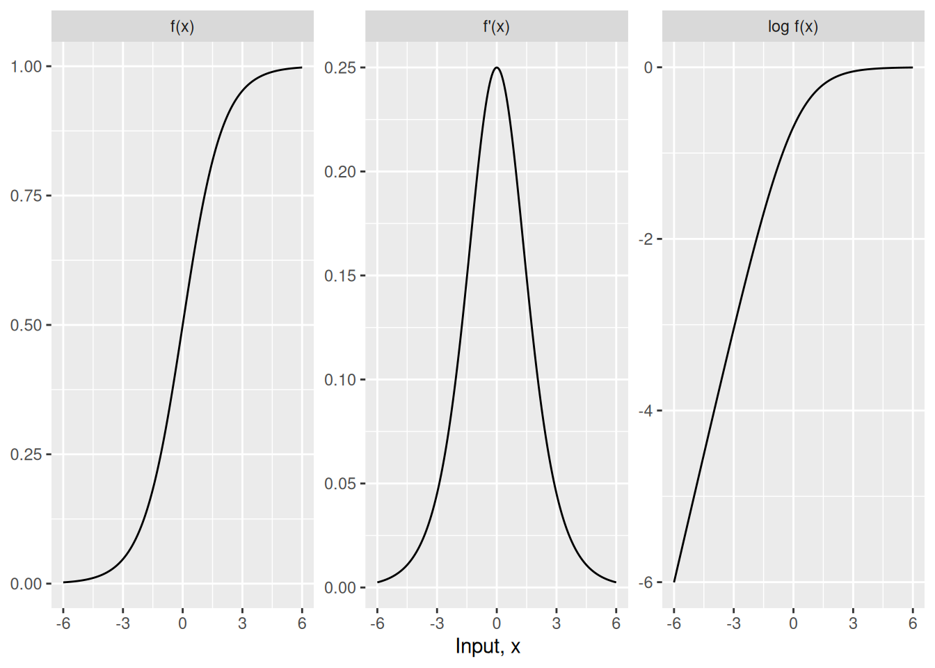
1.4 Tangent lines
DefDefinition 16 (Tangent line)
Definition 16 (Tangent line) Let \(f\) be differentiable at \(c\) (Definition 6). The tangent line to the graph of \(f\) at \(c\) is the graph of the affine function
\[x \mapsto f(c) + f'(c)\,(x - c),\]
the line through the point \((c, f(c))\) with slope \(f'(c)\). The slope \(f'(c)\) is also called the tangent slope of \(f\) at \(c\).
Example 9 (The tangent line to \(x^2\) at \(1\)) For \(f(x) = x^2\) at \(c = 1\), \(f(1) = 1\) and \(f'(1) = 2\) (Example 5), so the tangent line is the graph of
\[ \begin{aligned} x &\mapsto 1 + 2\,(x - 1) && \text{(substitute } f(1) = 1 \text{ and } f'(1) = 2 \text{)} \\ &= 2x - 1 && \text{(distribute, and } 1 - 2 = -1 \text{)} \end{aligned} \]
At \(x = 1.1\) the tangent line has height \(2(1.1) - 1 = 1.2\), close to the curve’s height \(f(1.1) = 1.21\); the gap, \(1.21 - 1.2 = 0.01\), is \((1.1 - 1)^2\).
1.5 Linear approximation
For a differentiable function \(f\) and a small step \(\varepsilon\),
\[f(w + \varepsilon) \approx f(w) + \varepsilon\,\frac{d }{d w}f(w) \tag{1}\]
DefDefinition 17 (Linear approximation (first-order Taylor approximation))
Definition 17 (Linear approximation (first-order Taylor approximation)) For a function \(f\) that is differentiable at \(w\), the linear approximation of \(f\) at \(w\) [14] (also called the first-order Taylor approximation) is the function of the step \(\varepsilon\)
\[\hat{f}_w(\varepsilon) = f(w) + \varepsilon\,\frac{d }{d w}f(w)\]
so Equation 1 says \(f(w + \varepsilon) \approx \hat{f}_w(\varepsilon)\) for small \(\varepsilon\). Figure 2 illustrates this approximation interactively for a quadratic function.
RemarkRemark 2 (The “linear” approximation is affine)
Remark 2 (The “linear” approximation is affine). The linear approximation \(\hat{f}_w\) (Definition 17) is an affine function of the step \(\varepsilon\): its slope is \(\frac{d }{d w}f(w)\) and its intercept is \(f(w)\). It is linear in \(\varepsilon\) only when \(f(w) = 0\). The name “linear approximation” uses “linear” in the looser sense of elementary algebra (remark). Boyd and Vandenberghe [15], section 2.2, treats the first-order Taylor approximation as an affine function for functions of several variables as well.
ExrExercise 13 (Tangent line approximation)
Exercise 13 (Tangent line approximation) Adapted from Miller [10], Question 1.1.8.
Let \(f(x) = 4x + \sqrt{2}\cos x\).
- Compute \(f'(x)\).
- Find the equation of the tangent line to the curve \(y = f(x)\) at \(x = \pi/4\).
- Use the tangent line to approximate \(f(\pi/4 + 0.01)\), and compare that approximation with the exact value.
1.6 Taylor series
DefDefinition 18 (Taylor polynomial)
Definition 18 (Taylor polynomial) Let \(f\) be a function that has at least \(n\) derivatives at a point \(x_0\). The Taylor polynomial of degree \(n\) for \(f\) centered at \(x_0\) is:
\[ \begin{aligned} P_n(x) &= \sum_{k=0}^n \frac{f^{(k)}(x_0)}{k!}(x - x_0)^k \\ &= f(x_0) + f'(x_0)(x - x_0) + \frac{f''(x_0)}{2!}(x - x_0)^2 + \dots + \frac{f^{(n)}(x_0)}{n!}(x - x_0)^n \end{aligned} \tag{2}\]
ExmExample 10 (Taylor series of the exponential function)
Example 10 (Taylor series of the exponential function) For \(f(x) = e^x\) centered at \(x_0 = 0\), every derivative is
\[ \begin{aligned} f^{(k)}(0) &= e^0 \\ &= 1. \end{aligned} \]
The degree-\(n\) Maclaurin polynomial is:
\[ \begin{aligned} P_n(x) &= 1 + x + \frac{x^2}{2!} + \dots + \frac{x^n}{n!} \\ &= \sum_{k=0}^n \frac{x^k}{k!} \end{aligned} \]
Because the remainder \(R_n(x) \to 0\) as \(n \to \infty\) for all \(x \in \mathbb{R}\), the Taylor series converges everywhere to \(e^x\):
\[e^x = \sum_{k=0}^\infty \frac{x^k}{k!}\]
DefDefinition 19 (Maclaurin polynomial)
Definition 19 (Maclaurin polynomial) When \(x_0 = 0\), the Taylor polynomial \(P_n(x)\) (Definition 18) is called the Maclaurin polynomial.
DefDefinition 20 (Taylor series)
Definition 20 (Taylor series) Let \(f\) and \(x_0\) be as in Definition 18. When \(f\) is infinitely differentiable and the series converges to \(f(x)\) on an open interval containing \(x_0\), the infinite sum \(\sum_{k=0}^\infty \frac{f^{(k)}(x_0)}{k!}(x - x_0)^k\) is the Taylor series of \(f\) centered at \(x_0\).
TipVideo
Chapter 11 of the Essence of calculus series by 3Blue1Brown develops the geometric and polynomial intuition behind Taylor approximations:
- Taylor series shows how higher-order derivatives match the curvature and rate of change of a function near a point to build polynomial approximations (Definition 18).
ExrExercise 14 (Taylor polynomial of a polynomial at the origin)
Exercise 14 (Taylor polynomial of a polynomial at the origin) Adapted from Miller [10], Question 1.1.16.
Find the first five terms (up to degree 4) of the Taylor series for
\[f(x) = x^8 + x^4 + 3\]
at \(x_0 = 0\).
ExrExercise 15 (Taylor expansion of a polynomial at a nonzero point)
Exercise 15 (Taylor expansion of a polynomial at a nonzero point) Adapted from Miller [10], Question 1.1.17.
Find the first three terms (up to degree 2) of the Taylor series for
\[f(x) = x^8 + x^4 + 3\]
at \(x_0 = 1\).
ExmExample 11 (Taylor series of the cosine function)
Example 11 (Taylor series of the cosine function) For \(f(x) = \cos x\) centered at \(x_0 = 0\), the derivatives follow a repeating cycle of length 4:
\[\begin{aligned} f(0) &= \cos(0) \\ &= 1, \\ f'(0) &= -\sin(0) \\ &= 0, \\ f''(0) &= -\cos(0) \\ &= -1, \\ f'''(0) &= \sin(0) \\ &= 0, \end{aligned}\]
and in general \(f^{(2k)}(0) = (-1)^k\) and \(f^{(2k+1)}(0) = 0\) for all \(k \ge 0\). The Taylor series (Maclaurin series) converges everywhere to \(\cos x\):
\[ \begin{aligned} \cos x &= 1 - \frac{x^2}{2!} + \frac{x^4}{4!} - \frac{x^6}{6!} + \dots \\ &= \sum_{k=0}^\infty \frac{(-1)^k}{(2k)!}x^{2k} \end{aligned} \]
ExmExample 12 (Taylor series of the sine function)
Example 12 (Taylor series of the sine function) For \(f(x) = \sin x\) centered at \(x_0 = 0\), the derivatives evaluate at \(0\) to \(f^{(2k)}(0) = 0\) and \(f^{(2k+1)}(0) = (-1)^k\) for all \(k \ge 0\). The Taylor series converges everywhere to \(\sin x\):
\[ \begin{aligned} \sin x &= x - \frac{x^3}{3!} + \frac{x^5}{5!} - \frac{x^7}{7!} + \dots \\ &= \sum_{k=0}^\infty \frac{(-1)^k}{(2k+1)!}x^{2k+1} \end{aligned} \]
ExrExercise 16 (Taylor expansion of a scaled cosine)
Exercise 16 (Taylor expansion of a scaled cosine) Adapted from Miller [10], Question 1.1.18.
Find the terms up to degree 4 in the Taylor series for
\[f(x) = \cos(5x)\]
at \(x_0 = 0\).
ExrExercise 17 (Taylor series of a power of a function)
Exercise 17 (Taylor series of a power of a function) Adapted from Miller [10], Question 1.1.19.
Find the terms up to degree 4 in the Taylor series for
\[f(x) = \cos^3(5x)\]
at \(x_0 = 0\).
ExrExercise 18 (Linear Taylor polynomial of the exponential)
Exercise 18 (Linear Taylor polynomial of the exponential) Adapted from Miller [10], Question 1.1.20.
Find the first two terms (degree 1) of the Taylor series for
\[f(x) = e^x\]
at \(x_0 = 0\).
ExrExercise 19 (Taylor series of a composite exponential)
Exercise 19 (Taylor series of a composite exponential) Adapted from Miller [10], Question 1.1.21.
Find the first six terms (up to degree 5) of the Taylor series for
\[f(x) = {\operatorname{exp}\mathopen{}\left\{x^8\right\}\mathclose{}}\]
at \(x_0 = 0\).
ExrExercise 20 (Taylor expansion of the normal density)
Exercise 20 (Taylor expansion of the normal density) Adapted from Miller [10], Question 1.1.22.
Find the terms up to degree 3 of the Taylor series for the standard normal density
\[\phi(x) = \frac{1}{\sqrt{2\pi}}{\operatorname{exp}\mathopen{}\left\{-\frac{x^2}{2}\right\}\mathclose{}}\]
at \(x_0 = 0\).
LemTheorem 13 (Maclaurin polynomial of the standard normal density)
Theorem 13 (Maclaurin polynomial of the standard normal density) The Maclaurin polynomial (Definition 19) of degree 3 of the standard normal density \(\phi(x) = \frac{1}{\sqrt{2\pi}}{\operatorname{exp}\mathopen{}\left\{-\frac{x^2}{2}\right\}\mathclose{}}\) is
\[P_3(x) = \frac{1}{\sqrt{2\pi}} - \frac{x^2}{2\sqrt{2\pi}}\]
ProofProof
Proof. This is the solution to Exercise 20, worked in Solution 20.
ExrExercise 21 (Taylor expansion of the square root)
Exercise 21 (Taylor expansion of the square root) Adapted from Miller [10], Question 1.1.23.
Find the first three terms (up to degree 2) of the Taylor series for
\[f(x) = \sqrt{x}\]
at \(x_0 = 1/3\).
ExrExercise 22 (Taylor expansion of a fractional power)
Exercise 22 (Taylor expansion of a fractional power) Adapted from Miller [10], Question 1.1.24.
Find the first three terms of the Taylor series for
\[f(x) = (1 + x)^{1/3}\]
at \(x_0 = 1/2\).
Exercise 23 (Taylor expansion of \(x \log x\)) Adapted from Miller [10], Question 1.1.25.
Find the first three terms (up to degree 2) of the Taylor series for
\[f(x) = x\log x\]
at \(x_0 = 1\).
Exercise 24 (Maclaurin series of \(\log(1 + x)\)) Adapted from Miller [10], Question 1.1.26.
Find the first three terms of the Taylor series for
\[f(x) = \log(1 + x)\]
at \(x_0 = 0\).
Theorem 14 (Maclaurin polynomial of \(\log(1 + x)\)) The Maclaurin polynomial (Definition 19) of degree 3 of \(f(x) = \log(1 + x)\) is
\[P_3(x) = x - \frac{x^2}{2} + \frac{x^3}{3}\]
ProofProof
Proof. This is the solution to Exercise 24, worked in Solution 24.
Exercise 25 (Maclaurin series of \(\log(1 - x)\)) Adapted from Miller [10], Question 1.1.27.
Find the terms up to degree 3 of the Taylor series for
\[f(x) = \log(1 - x)\]
at \(x_0 = 0\).
Theorem 15 (Maclaurin polynomial of \(\log(1 - x)\)) The Maclaurin polynomial (Definition 19) of degree 3 of \(f(x) = \log(1 - x)\) is
\[P_3(x) = -x - \frac{x^2}{2} - \frac{x^3}{3}\]
ProofProof
Proof. This is the solution to Exercise 25, worked in Solution 25.
Exercise 26 (Taylor series of \(\log((1 - x)e^x)\)) Adapted from Miller [10], Question 1.1.28.
Find the first two non-zero terms of the Taylor series for
\[f(x) = \log((1 - x)e^x)\]
at \(x_0 = 0\).
ExrExercise 27 (Taylor series of a product of known expansions)
Exercise 27 (Taylor series of a product of known expansions) Adapted from Miller [10], Question 1.1.29.
Find the terms up to degree 2 of the Taylor series for
\[f(x) = \cos(x)\log(1 + x)\]
at \(x_0 = 0\).
Exercise 28 (Taylor series of \(\log(1 + 2x)\)) Adapted from Miller [10], Question 1.1.30.
Find the first two non-zero terms of the Taylor series for
\[f(x) = \log(1 + 2x)\]
at \(x_0 = 0\).
References
[1]
Wikipedia contributors, “Limit of a function — Wikipedia, the free encyclopedia.” 2026. Available: https://en.wikipedia.org/wiki/Limit_of_a_function
[2]
Wikipedia contributors, “One-sided limit — Wikipedia, the free encyclopedia.” 2026. Available: https://en.wikipedia.org/wiki/One-sided_limit
[3]
Wikipedia contributors, “Difference quotient — Wikipedia, the free encyclopedia.” 2026. Available: https://en.wikipedia.org/wiki/Difference_quotient
[4]
Wikipedia contributors, “Differentiable function — Wikipedia, the free encyclopedia.” 2026. Available: https://en.wikipedia.org/wiki/Differentiable_function
[5]
R. Larson and B. H. Edwards, Calculus, 11th ed. Boston, MA: Cengage Learning, 2018. Available: https://www.cengage.com/c/calculus-11e-larson/
[6]
Wikipedia contributors, “Derivative — Wikipedia, the free encyclopedia.” 2026. Available: https://en.wikipedia.org/wiki/Derivative
[7]
Wikipedia contributors, “Notation for differentiation — Wikipedia, the free encyclopedia.” 2026. Available: https://en.wikipedia.org/wiki/Notation_for_differentiation
[8]
Wikipedia contributors, “Second derivative — Wikipedia, the free encyclopedia.” 2026. Available: https://en.wikipedia.org/wiki/Second_derivative
[9]
Wikipedia contributors, “Power rule — Wikipedia, the free encyclopedia.” 2026. Available: https://en.wikipedia.org/wiki/Power_rule
[10]
S. J. Miller, The probability lifesaver: Calculus review problems. 2016. Available: https://web.williams.edu/Mathematics/sjmiller/public_html/probabilitylifesaver/index.htm#:~:text=http%3A//web.williams.edu/Mathematics/sjmiller/public_html/probabilitylifesaver/supplementalchap_calcreview.pdf
[11]
Wikipedia contributors, “Product rule — Wikipedia, the free encyclopedia.” 2026. Available: https://en.wikipedia.org/wiki/Product_rule
[12]
Wikipedia contributors, “Quotient rule — Wikipedia, the free encyclopedia.” 2026. Available: https://en.wikipedia.org/wiki/Quotient_rule
[13]
Wikipedia contributors, “Chain rule — Wikipedia, the free encyclopedia.” 2026. Available: https://en.wikipedia.org/wiki/Chain_rule
[14]
Wikipedia contributors, “Linear approximation — Wikipedia, the free encyclopedia.” 2026. Available: https://en.wikipedia.org/wiki/Linear_approximation
[15]
S. Boyd and L. Vandenberghe, Introduction to applied linear algebra: Vectors, matrices, and least squares. Cambridge University Press, 2018. doi: 10.1017/9781108583664.