Integrals and the Fundamental Theorem of Calculus
1 Integration
Integration is the inverse operation of differentiation: it recovers a function from its derivative and accumulates quantities such as areas, totals, and probabilities. We begin with antiderivatives, then state basic integration rules, and conclude with the Fundamental Theorem of Calculus and a worked example from probability.
TipVideos
Jon Krohn’s “Calculus for Machine Learning” YouTube playlist introduces integral calculus:
1.1 Antiderivatives
DefDefinition 1 (Antiderivative)
Definition 1 (Antiderivative) A function \(F\) is an antiderivative of \(f\) on an interval \(I\) [1] if:
\[\frac{\partial}{\partial x} F(x) = f(x), \quad \forall x \in I\]
Finding an antiderivative of \(f\) is called antidifferentiation, or antidifferentiating \(f\).
[2, Sec. 4.1], pp. 248–249
DefDefinition 2 (Indefinite integral)
Definition 2 (Indefinite integral) The indefinite integral of \(f\) [1] is the family of all antiderivatives (Definition 1) of \(f\):
\[\int f(x)\,dx = F(x) + C\]
where \(F\) is any one antiderivative of \(f\) and \(C\) is an arbitrary constant of integration.
[2, Sec. 4.1], pp. 248–249
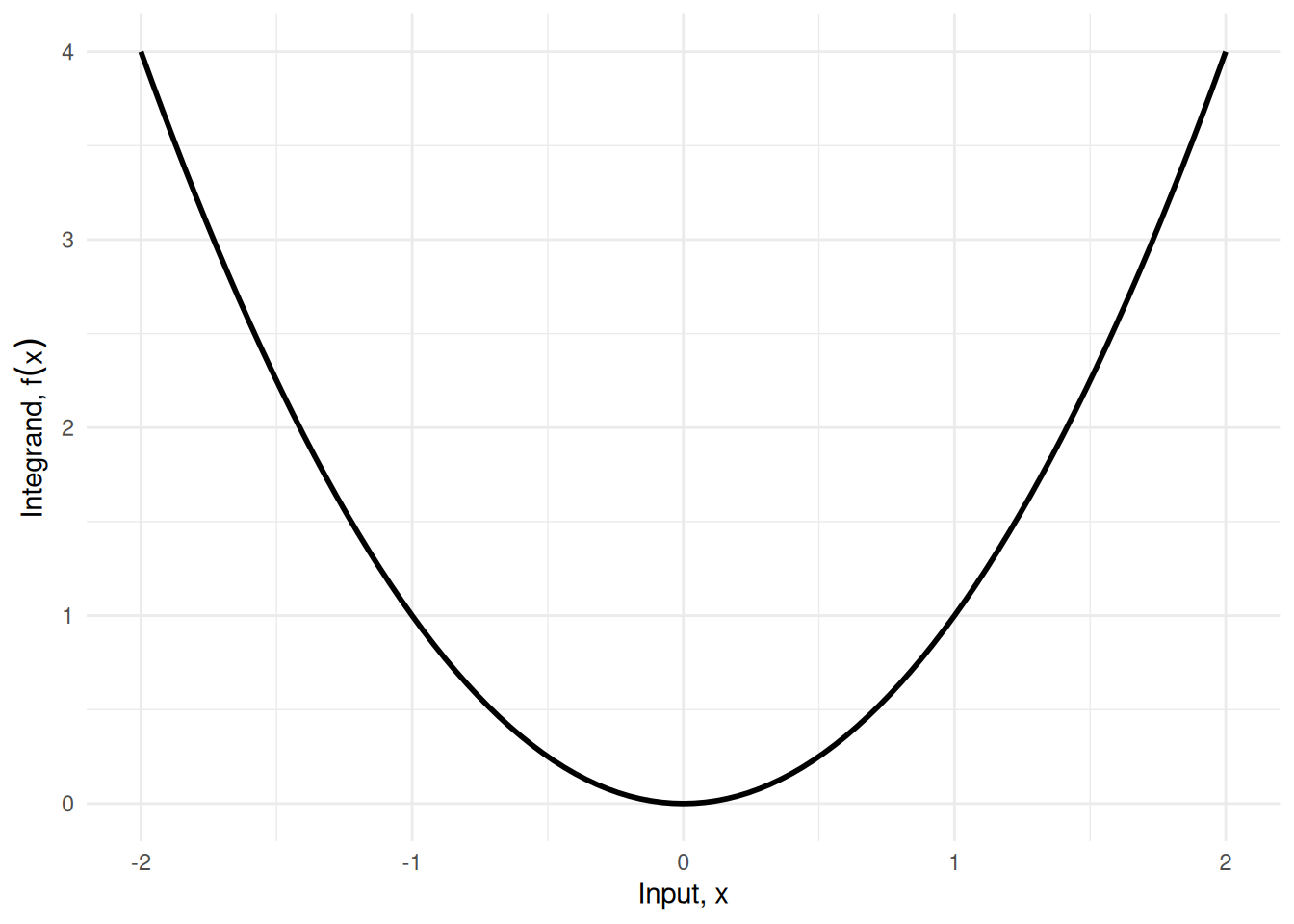
Example 1 (Antiderivative of \(x^2\)) For \(f(x) = x^2\), an antiderivative is \(F(x) = \frac{x^3}{3}\), since
\[ \begin{aligned} \frac{\partial}{\partial x}\frac{x^3}{3} &= x^2 \\ &= f(x). \end{aligned} \]
Adding any constant \(C\) gives another antiderivative; for example, with \(C = 7\), \(F(x) = \frac{x^3}{3} + 7\) also satisfies \(F'(x) = x^2\), since adding a constant does not change the derivative. \(G(x) = x^3\) is not an antiderivative of \(x^2\): \(G'(x) = 3x^2 \ne x^2\) for \(x \ne 0\).
See Figure 1.
Show R code
ggplot2::ggplot() +
  ggplot2::geom_function(fun = \(x) x^2, xlim = x_lim, linewidth = 1) +
  ggplot2::labs(x = "Input, x", y = expression("Integrand, " * f(x))) +
ggplot2::theme_minimal()Show R code
x_seq <- seq(x_lim[1], x_lim[2], length.out = 200)
df <- C_vals |>
  lapply(\(C) {
    tibble::tibble(
      x = x_seq,
      y = x_seq^3 / 3 + C,
      C = factor(C)
    )
  }) |>
  dplyr::bind_rows()

ggplot2::ggplot(df, ggplot2::aes(x = x, y = y, color = C)) +
  ggplot2::geom_line(linewidth = 0.8) +
  ggplot2::labs(
    x = "Input, x",
    y = expression("Antiderivative, " * F(x)),
    color = "C"
  ) +
  ggplot2::theme_minimal()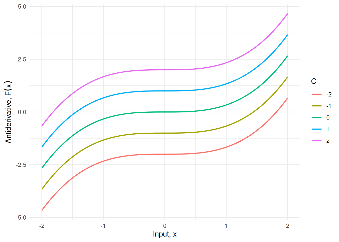
LemTheorem 1 (Basic integration rules)
Theorem 1 (Basic integration rules) Each antiderivative in the table is defined only up to an arbitrary constant \(C\) (see Definition 1); the table omits \(+ C\) from every row for brevity.
| Function \(f(x)\) | Antiderivative \(F(x)\) | Condition |
|---|---|---|
| \(c\) | \(cx\) | — |
| \(x^n\) | \(\dfrac{x^{n+1}}{n+1}\) | \(n \ne -1\) |
| \(\dfrac{1}{x}\) | \({\operatorname{log}\mathopen{}\left\{\mathopen{}\left|x\right|\mathclose{}\right\}\mathclose{}}\) | \(x \ne 0\) |
| \(\text{e}^{x}\) | \(\text{e}^{x}\) | (self-antiderivative) |
| \(\text{e}^{cx}\) | \(\dfrac{1}{c}\text{e}^{cx}\) | \(c \ne 0\) |
| \(\sin x\) | \(-\cos x\) | — |
| \(\cos x\) | \(\sin x\) | — |
| \(c \cdot f(x)\) | \(c \cdot F(x)\) | — |
| \(f(x) + g(x)\) | \(F(x) + G(x)\) | — |
The first two rows, the trigonometric rows (\(\sin x\), \(\cos x\)), and the bottom two rows (linearity) are from [2, Sec. 4.1], p. 250 “Basic Integration Rules”; \(1/x\) is from [2, Sec. 5.2], Theorem 5.5, p. 324; \(\text{e}^{x}\) and \(\text{e}^{cx}\) are from [2, Sec. 5.4], Theorem 5.12, p. 346.
Example 2 (Antiderivative of \(3x^2 - 1\)) By the power rule (\(n = 2\)) and linearity from Theorem 1:
\[ \begin{aligned} \int \mathopen{}\left(3x^2 - 1\right)\mathclose{}\,dx &= 3 \cdot\frac{x^3}{3} - x + C \\ &= x^3 - x + C. \end{aligned} \]
Verify by differentiating:
\[ \begin{aligned} \frac{\partial}{\partial x}\mathopen{}\left(x^3 - x + C\right)\mathclose{} &= 3x^2 - 1 \\ &= f(x), \end{aligned} \]
as required.
TipVideos
Jon Krohn’s “Calculus for Machine Learning” YouTube playlist has videos on these rules:
1.2 Regularity Conditions
DefDefinition 3 (Differentiable on an interval)
Definition 3 (Differentiable on an interval) A function \(f\) is differentiable on an interval if it is differentiable (Definition 6 in Derivatives and Taylor Series) at every point of the interval other than its endpoints, and, at each endpoint that belongs to the interval, it has the one-sided derivative (Definition 12 in Derivatives and Taylor Series) from inside the interval: the right-hand derivative at the left endpoint and the left-hand derivative at the right endpoint.
[2, Sec. 2.1], p. 100
ExmExample 3 (Differentiable on one interval but not another)
Example 3 (Differentiable on one interval but not another)
- \(f(x) = x^2\) is differentiable on \([0, 1]\): the computation of Example 4 in Derivatives and Taylor Series with \(3\) replaced by any \(c\) gives \(\tfrac{f(c + h) - f(c)}{h} = 2c + h\), which tends to \(2c\), including the one-sided limits at the endpoints \(0\) and \(1\).
- \(g(x) = \sqrt[3]{x}\) is differentiable on \([1, 2]\), but not on \([-1, 1]\): the point \(0\) is in \([-1, 1]\) and is not an endpoint, and Example 4 in Derivatives and Taylor Series shows \(g\) is not differentiable there.
DefDefinition 4 (Continuous function)
Definition 4 (Continuous function) A function \(f\) is continuous at \(x = c\) [3] if all three conditions hold:
- \(f(c)\) is defined,
- \(\lim_{x \to c} f(x)\) exists, and
- \(\lim_{x \to c} f(x) = f(c)\).
[2, Sec. 1.4], p. 73
DefDefinition 5 (Discontinuous function)
Definition 5 (Discontinuous function) If any of the three conditions of Definition 4 fails, \(f\) is discontinuous at \(c\).
[2, Sec. 1.4], p. 73
ExmExample 4 (A continuous function, and one failure of each condition)
Example 4 (A continuous function, and one failure of each condition)
-
\(f(x) = x^2\) is continuous at \(c = 1\): \(f(1) = 1\) is defined, and
\[ \begin{aligned} \lim_{x \to 1} x^2 &= 1 \\ &= f(1). \end{aligned} \]
-
\(g(x) = \tfrac{x^2 - 1}{x - 1}\) fails condition 1 at \(c = 1\): \(g(1)\) is not defined (it would divide by zero), even though
\[ \begin{aligned} \lim_{x \to 1} g(x) &= \lim_{x \to 1} (x + 1) \\ &= 2 \end{aligned} \]
exists (\(x^2 - 1 = (x - 1)(x + 1)\), and the factor \(x - 1\) cancels for \(x \ne 1\)).
The step function \(H(x) = 1\) for \(x \ge 0\) and \(H(x) = 0\) for \(x < 0\) fails condition 2 at \(c = 0\): values to the left are all \(0\) and values to the right are all \(1\), so \(\lim_{x \to 0} H(x)\) does not exist.
\(k(x) = x^2\) for \(x \ne 1\), with \(k(1) = 5\), fails condition 3 at \(c = 1\): \(\lim_{x \to 1} k(x) = 1\) exists but differs from \(k(1) = 5\).
DefDefinition 6 (Jump discontinuity)
Definition 6 (Jump discontinuity) A function \(f\) has a jump discontinuity at \(c\) [4] if both one-sided limits (Definition 4 in Derivatives and Taylor Series) \(\lim_{x \to c^-} f(x)\) and \(\lim_{x \to c^+} f(x)\) exist but are not equal. Then \(\lim_{x \to c} f(x)\) does not exist, so \(f\) is discontinuous at \(c\) (Definition 5).
ExmExample 5 (A jump discontinuity, and a discontinuity that is not a jump)
Example 5 (A jump discontinuity, and a discontinuity that is not a jump)
- The step function \(H\) of Example 2 in Derivatives and Taylor Series has a jump discontinuity at \(0\): \(\lim_{x \to 0^-} H(x) = 0\) and \(\lim_{x \to 0^+} H(x) = 1\) both exist, and \(0 \ne 1\). The size of the jump is \(1 - 0 = 1\).
- \(g(x) = \tfrac{x^2 - 1}{x - 1}\) of Example 4 is discontinuous at \(1\), because \(g(1)\) is not defined, but it does not have a jump discontinuity there: for \(x \ne 1\), \(g(x) = x + 1\), so both one-sided limits at \(1\) equal \(1 + 1 = 2\).
DefDefinition 7 (Continuous on a closed interval)
Definition 7 (Continuous on a closed interval) A function \(f\) is continuous on a closed interval \([a, b]\) if all three conditions hold:
- \(f\) is continuous (Definition 4) at every point of the open interval \((a, b)\),
- \(\lim_{x \to a^+} f(x) = f(a)\), and
- \(\lim_{x \to b^-} f(x) = f(b)\).
[2, Sec. 1.4], p. 73
Example 6 (Continuity on \(\lbrack 0, 1\rbrack\) uses one-sided limits at the endpoints) Let \(f(x) = \sqrt{x}\), the square root, defined for \(x \ge 0\). Because \(f\) is undefined for \(x < 0\), only the right-hand limit of \(f\) at \(0\) makes sense, and Definition 7 asks only for that one-sided limit at the endpoint \(0\). Here \(f\) is continuous at every point of \((0, 1)\),
\[ \begin{aligned} \lim_{x \to 0^+} \sqrt{x} &= 0 \\ &= f(0), \end{aligned} \]
and
\[ \begin{aligned} \lim_{x \to 1^-} \sqrt{x} &= 1 \\ &= f(1), \end{aligned} \]
so \(f\) is continuous on \([0, 1]\) (Definition 7).
Example 7 (A function not continuous on \(\lbrack 0, 1\rbrack\)) Let \(f(x) = 0\) for \(0 \le x < 1\) and \(f(1) = 2\). Conditions 1 and 2 of Definition 7 hold, but
\[ \begin{aligned} \lim_{x \to 1^-} f(x) &= 0 \\ &\ne 2 \\ &= f(1), \end{aligned} \]
so condition 3 fails and \(f\) is not continuous on \([0, 1]\).
DefDefinition 8 (Partition of an interval)
Definition 8 (Partition of an interval) A partition \(\mathcal{P}\) of a closed interval \([a, b]\) [5] is a finite list of points
\[ \begin{aligned} a &= x_0 \\ &< x_1 \\ &< \cdots \\ &< x_n \\ &= b. \end{aligned} \]
It splits \([a, b]\) into the \(n\) subintervals \([x_{i-1}, x_i]\), of widths \(\Delta x_i \stackrel{\text{def}}{=}x_i - x_{i-1}\).
Example 8 (A partition of \(\lbrack 0, 1\rbrack\)) The points \(0 < 0.25 < 0.5 < 1\) form a partition of \([0, 1]\) with \(n = 3\) subintervals, of widths \(\Delta x_1 = 0.25\), \(\Delta x_2 = 0.25\), and \(\Delta x_3 = 0.5\).
Example 9 (Lists that are not partitions of \(\lbrack 0, 1\rbrack\))
- \(0, 0.5, 0.25, 1\) is not a partition: the points are not increasing, since \(0.5 > 0.25\).
- \(0 < 0.5\) is not a partition of \([0, 1]\): its last point is \(0.5\), not \(b = 1\).
DefDefinition 9 (Mesh of a partition)
Definition 9 (Mesh of a partition) The mesh of a partition \(\mathcal{P}\) (Definition 8) is its largest subinterval width,
\[\mathopen{}\left\lVert\mathcal{P}\right\rVert\mathclose{} \stackrel{\text{def}}{=}\max_{i \in \mathopen{}\left\{1, \ldots, n\right\}\mathclose{}} \Delta x_i,\]
where \(n\) is the number of subintervals of \(\mathcal{P}\).
Example 10 (The mesh of a partition of \(\lbrack 0, 1\rbrack\)) For the partition of \([0, 1]\) in Example 8, with widths \(\Delta x_1 = 0.25\), \(\Delta x_2 = 0.25\), and \(\Delta x_3 = 0.5\), the mesh is the largest of these widths, \(\mathopen{}\left\lVert\mathcal{P}\right\rVert\mathclose{} = 0.5\).
DefDefinition 10 (Sample point)
Definition 10 (Sample point) For a partition \(\mathcal{P}\) of \([a, b]\) (Definition 8), choose a sample point \(x_i^*\) in each subinterval \([x_{i-1}, x_i]\).
DefDefinition 11 (Riemann sum)
Definition 11 (Riemann sum) Let \(f\) be a function on \([a, b]\), let \(\mathcal{P}\) be a partition
\[ \begin{aligned} a &= x_0 \\ &< x_1 \\ &< \cdots \\ &< x_n \\ &= b \end{aligned} \]
of \([a, b]\) (Definition 8), and choose a sample point \(x_i^*\) (Definition 10) in each subinterval \([x_{i-1}, x_i]\). The Riemann sum of \(f\) for \(\mathcal{P}\) [6] and these sample points is
\[\sum_{i=1}^nf(x_i^*)\,\Delta x_i,\]
where \(\Delta x_i = x_i - x_{i-1}\).
Example 11 (A Riemann sum for \(x^2\) on \(\lbrack 0, 1\rbrack\)) Let \(f(x) = x^2\), take the partition \(0 < 0.25 < 0.5 < 1\) of Example 8, with widths \(\Delta x_1 = 0.25\), \(\Delta x_2 = 0.25\), and \(\Delta x_3 = 0.5\), and take each sample point at the right end of its subinterval: \(x_1^* = 0.25\), \(x_2^* = 0.5\), and \(x_3^* = 1\). Then
\[ \begin{aligned} \sum_{i=1}^{3} f(x_i^*)\,\Delta x_i &= f(0.25) \cdot 0.25 + f(0.5) \cdot 0.25 + f(1) \cdot 0.5 && \text{(write out the three terms)} \\ &= 0.0625 \cdot 0.25 + 0.25 \cdot 0.25 + 1 \cdot 0.5 && \text{(evaluate } f(x) = x^2 \text{)} \\ &= 0.015625 + 0.0625 + 0.5 && \text{(multiply)} \\ &= 0.578125 && \text{(add)} \end{aligned} \]
DefDefinition 12 (Riemann integral (definite integral))
Definition 12 (Riemann integral (definite integral)) Let \(f\) be a bounded function on \([a, b]\). For each partition \(\mathcal{P}\) of \([a, b]\) (Definition 8), choose a sample point \(x_i^*\) in each subinterval \([x_{i-1}, x_i]\). The Riemann integral of \(f\) over \([a, b]\) [7] (also called the definite integral of \(f\) from \(a\) to \(b\)) is the limit of the Riemann sums (Definition 11) as the mesh (Definition 9) shrinks to zero:
\[\int_a^b f(x)\,dx \stackrel{\text{def}}{=}\lim_{\mathopen{}\left\lVert\mathcal{P}\right\rVert\mathclose{} \to 0} \sum_{i=1}^nf(x_i^*)\,\Delta x_i,\]
when that limit exists and has the same value for every choice of the partitions and of the sample points \(x_i^*\).
[2, Sec. 4.3], p. 272
DefDefinition 13 (Riemann integrable)
Definition 13 (Riemann integrable) A bounded function \(f\) is Riemann integrable on \([a, b]\) if the Riemann sums (Definition 11) \(\sum_{i=1}^nf(x_i^*)\,\Delta x_i\), over partitions \(\mathcal{P}\) of \([a, b]\) (Definition 8) with a sample point \(x_i^*\) in each subinterval \([x_{i-1}, x_i]\), approach a real-number limit as the mesh \(\mathopen{}\left\lVert\mathcal{P}\right\rVert\mathclose{}\) (Definition 9) shrinks to zero, and that limit is the same for every choice of the partitions and of the sample points.
[2, Sec. 4.3], p. 272
ExmExample 12 (A constant function is integrable)
Example 12 (A constant function is integrable) Let \(f(x) = 2\) on \([0, 3]\). For every partition and every choice of sample points,
\[ \begin{aligned} \sum_{i=1}^nf(x_i^*)\,\Delta x_i &= \sum_{i=1}^n2\,\Delta x_i && \text{(} f \text{ is } 2 \text{ everywhere)} \\ &= 2 \sum_{i=1}^n\Delta x_i && \text{(factor out the constant)} \\ &= 2 \cdot(3 - 0) && \text{(the widths add up to the length of } [0, 3] \text{)} \\ &= 6, && \text{(multiply)} \end{aligned} \]
so the sums have the same limit, \(6\), for every choice: \(f\) is Riemann integrable on \([0, 3]\) (Definition 13), and \(\int_0^3 2\,dx = 6\) (Definition 12).
DefDefinition 14 (Integrand)
Definition 14 (Integrand) In an integral such as \(\int_a^b f(x)\,dx\) (Definition 12) or \(\int f(x)\,dx\) (Definition 2), the function \(f\) being integrated is the integrand.
ExmExample 13 (Integrands)
Example 13 (Integrands)
- In \(\int_0^3 2\,dx = 6\) (Example 12), the integrand is the constant function \(f(x) = 2\), and the limits of integration are \(0\) and \(3\).
- In \(\int \mathopen{}\left(3x^2 - 1\right)\mathclose{}\,dx = x^3 - x + C\) (Example 2), the integrand is \(f(x) = 3x^2 - 1\); its value at \(x = 2\) is \(3 \cdot 4 - 1 = 11\).
RemarkRemark 1 (Riemann integrable functions and Riemann integrals)
Remark 1 (Riemann integrable functions and Riemann integrals). A bounded function \(f\) is Riemann integrable on \([a, b]\) exactly when its Riemann integral \(\int_a^b f(x)\,dx\) (Definition 12) exists; the integral is the common limit of the sums. For example, let \(g(x) = 1\) when \(x\) is rational and \(g(x) = 0\) when \(x\) is irrational, on \([0, 1]\). Every subinterval contains both rational and irrational points. Choosing every sample point rational gives \(\sum_{i=1}^n1 \cdot\Delta x_i = 1\) for every partition, because the widths \(\Delta x_i\) add up to the length \(1 - 0 = 1\) of \([0, 1]\), and choosing every sample point irrational gives \(\sum_{i=1}^n0 \cdot\Delta x_i = 0\). The two limits differ, so \(g\) is not Riemann integrable on \([0, 1]\), and \(\int_0^1 g(x)\,dx\) does not exist.
DefDefinition 15 (Equal-width Riemann sum)
Definition 15 (Equal-width Riemann sum) For a bounded function \(f\) on \([a, b]\) and a positive integer \(n\), split \([a, b]\) into \(n\) subintervals of equal width \(\Delta x \stackrel{\text{def}}{=}(b - a)/n\), and let \(x_i^*\) be any point in the \(i\)-th subinterval. The equal-width Riemann sum is
\[S_n \stackrel{\text{def}}{=}\sum_{i=1}^nf(x_i^*)\,\Delta x.\]
ExmExample 14 (An equal-width Riemann sum)
Example 14 (An equal-width Riemann sum) Let \(f(x) = x^2\) on \([0, 1]\), with \(n = 2\), so \(\Delta x = 1/2\), and take each sample point at the right end of its subinterval: \(x_1^* = \frac{1}{2}\) and \(x_2^* = 1\). Then
\[ \begin{aligned} S_2 &= f\mathopen{}\left(\tfrac{1}{2}\right)\mathclose{} \cdot\tfrac{1}{2} + f(1) \cdot\tfrac{1}{2} && \text{(equal-width Riemann sum with } n = 2 \text{)} \\ &= \tfrac{1}{4} \cdot\tfrac{1}{2} + 1 \cdot\tfrac{1}{2} && \text{(evaluate } f(x) = x^2 \text{)} \\ &= \tfrac{5}{8} && \text{(add)} \end{aligned} \]
TipVideos
Jon Krohn’s “Calculus for Machine Learning” YouTube playlist has videos on approximating an area by a sum of simple pieces, as a Riemann sum does, and on computing such sums in Python:
Before stating the Fundamental Theorem of Calculus, we record two prerequisite results. The usual statement of the Fundamental Theorem of Calculus assumes that the integrand \(f\) is continuous on \([a, b]\); continuity is sufficient there, though not necessary. The two results are “differentiability implies continuity”, which says where continuity comes from, and “continuity implies integrability”, which says what continuity gives us.
LemTheorem 2 (Differentiability implies continuity)
Theorem 2 (Differentiability implies continuity) If \(f\) is differentiable at \(x = c\), then \(f\) is continuous at \(x = c\).
[2], Theorem 2.1, p. 106
ProofProof
Proof. Because \(f'(c)\) exists, \(f(c)\) is defined, and:
\[ \begin{aligned} \lim_{h \to 0} \mathopen{}\left(f(c + h) - f(c)\right)\mathclose{} &= \lim_{h \to 0} \mathopen{}\left(\frac{f(c + h) - f(c)}{h} \cdot h\right)\mathclose{} && \text{(multiply and divide by } h \neq 0 \text{)} \\ &= \mathopen{}\left(\lim_{h \to 0} \frac{f(c + h) - f(c)}{h}\right)\mathclose{} \cdot\mathopen{}\left(\lim_{h \to 0} h\right)\mathclose{} && \text{(limit of a product, both limits exist)} \\ &= f'(c) \cdot 0 && \text{(definition of } f'(c) \text{)} \\ &= 0 && \text{(multiply)} \end{aligned} \]
So \(\lim_{h \to 0} f(c + h) = f(c)\), which is \(\lim_{x \to c} f(x) = f(c)\) with \(x = c + h\); all three conditions of Definition 4 hold.
Example 15 (Differentiable, hence continuous: \(x^3 - x\)) \(f(x) = x^3 - x\) is differentiable everywhere (with derivative \(f'(x) = 3x^2 - 1\)), so by Theorem 2 it is continuous everywhere.
Example 16 (Continuous but not differentiable: \(\mathopen{}\left|x\right|\mathclose{}\)) The absolute-value function \(f(x) = \mathopen{}\left|x\right|\mathclose{}\) is continuous at \(x = 0\), since
\[ \begin{aligned} \lim_{x \to 0}\mathopen{}\left|x\right|\mathclose{} &= 0 \\ &= \mathopen{}\left|0\right|\mathclose{}, \end{aligned} \]
but it is not differentiable at \(x = 0\): its left-hand derivative there is \(-1\) and its right-hand derivative is \(+1\) (Example 6 in Derivatives and Taylor Series).
This counterexample shows that the converse of Theorem 2 fails: continuity does not imply differentiability. See Figure 2.
Show R code
ggplot2::ggplot() +
  ggplot2::geom_function(fun = abs, xlim = c(-2, 2), linewidth = 1) +
  ggplot2::geom_point(ggplot2::aes(x = 0, y = 0), size = 3) +
  ggplot2::labs(x = "x", y = expression(f(x) == abs(x))) +
  ggplot2::theme_minimal()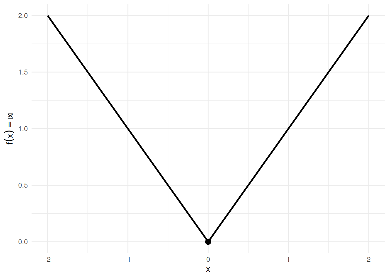
LemTheorem 3 (Continuity implies integrability)
Theorem 3 (Continuity implies integrability) If \(f\) is continuous on the closed interval \([a, b]\), then \(f\) is integrable on \([a, b]\) (i.e., the Riemann integral \(\int_a^b f(x)\,dx\) exists and is finite).
[2], Theorem 4.4, p. 272
ExmExample 17 (Continuous, hence integrable: polynomials)
Example 17 (Continuous, hence integrable: polynomials) Every polynomial is continuous on \(\mathbb{R}\), so by Theorem 3 every polynomial is integrable on every closed interval \([a, b]\).
ExmExample 18 (Integrable but not continuous: a step function)
Example 18 (Integrable but not continuous: a step function) Let \(f(x) = 0\) for \(x < \tfrac{1}{2}\) and \(f(x) = 1\) for \(x \ge \tfrac{1}{2}\). Then \(f\) has a jump discontinuity (Definition 6) at \(x = \tfrac{1}{2}\), but it is integrable on \([0, 1]\):
\[ \begin{aligned} \int_0^1 f(x)\,dx &= \int_0^{1/2} 0\,dx + \int_{1/2}^1 1\,dx \\ &= 0 + \tfrac{1}{2} \\ &= \tfrac{1}{2}. \end{aligned} \]
This counterexample shows that the converse of Theorem 3 fails: integrability does not imply continuity. See Figure 3.
Show R code
step_df <- tibble::tibble(
  x = c(0, 0.5, 0.5, 1),
  y = c(0, 0, 1, 1),
  segment = c("left", "left", "right", "right")
)

ggplot2::ggplot() +
  ggplot2::geom_rect(
    ggplot2::aes(xmin = 0.5, xmax = 1, ymin = 0, ymax = 1),
    fill = "steelblue", alpha = 0.3
  ) +
  ggplot2::geom_line(
    data = step_df,
    ggplot2::aes(x = x, y = y, group = segment),
    linewidth = 1
  ) +
  ggplot2::geom_point(ggplot2::aes(x = 0.5, y = 0), shape = 1, size = 3) +
  ggplot2::geom_point(ggplot2::aes(x = 0.5, y = 1), shape = 16, size = 3) +
  ggplot2::scale_x_continuous(
    breaks = c(0, 0.5, 1),
    labels = c("0", "1/2", "1")
  ) +
  ggplot2::scale_y_continuous(limits = c(-0.1, 1.2)) +
  ggplot2::labs(x = "x", y = "f(x)") +
  ggplot2::theme_minimal()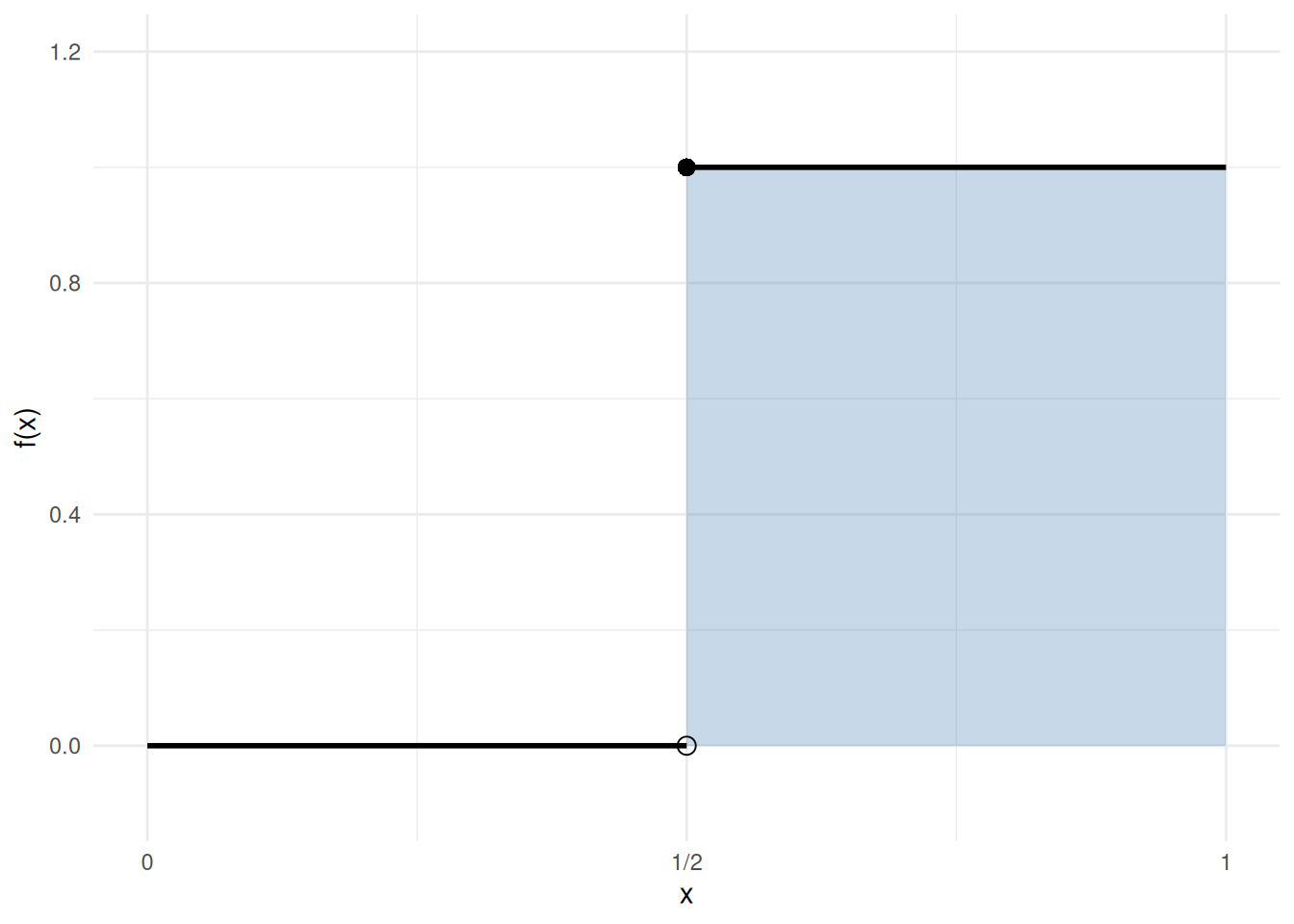
Together, Theorem 2 and Theorem 3 establish the chain:
\[\text{differentiable on } [a, b] \;\Rightarrow\; \text{continuous on } [a, b] \;\Rightarrow\; \text{integrable on } [a, b]\]
Example 16 and Example 18 show that neither implication reverses in general.
LemTheorem 4 (Equal-width Riemann sums converge to the integral)
Theorem 4 (Equal-width Riemann sums converge to the integral) If \(f\) is Riemann integrable on \([a, b]\) (Definition 13), then for every choice of the sample points \(x_i^*\), the equal-width Riemann sums (Definition 15) converge to the integral:
\[\lim_{n \to \infty} S_n = \int_a^b f(x)\,dx.\]
ProofProof
Proof. The \(n\) equal-width subintervals form a partition of \([a, b]\) whose mesh (Definition 9) is \((b - a)/n\), which goes to \(0\) as \(n \to \infty\). So \(S_n\) is one of the sums in the limit that defines the integral (Definition 12), along a sequence of partitions whose mesh goes to \(0\), and a limit that has the same value for every choice of partitions has that value along this sequence too.
Example 19 (Equal-width sums for \(\int_0^1 x\,dx\)) Let \(f(x) = x\) on \([0, 1]\), which is continuous and so Riemann integrable (Theorem 3), and take each sample point at the right end of its subinterval, \(x_i^* = i/n\). With \(\Delta x = 1/n\):
\[ \begin{aligned} S_n &= \sum_{i=1}^n\frac{i}{n} \cdot\frac{1}{n} && \text{(equal-width Riemann sum with } x_i^* = i/n \text{)} \\ &= \frac{1}{n^2} \sum_{i=1}^ni && \text{(factor out } 1/n^2 \text{)} \\ &= \frac{1}{n^2} \cdot\frac{n(n+1)}{2} && \text{(sum of the first } n \text{ integers)} \\ &= \frac{n+1}{2n} && \text{(cancel one factor of } n \text{)} \end{aligned} \]
So \(S_{10} = 0.55\), \(S_{100} = 0.505\), \(S_{1000} = 0.5005\), and \(S_n \to \frac{1}{2}\) as \(n \to \infty\). By Theorem 4, \(\int_0^1 x\,dx = \frac{1}{2}\).
1.3 Fundamental Theorem of Calculus
DefDefinition 16 (Accumulation function)
Definition 16 (Accumulation function) Let \(f\) be Riemann integrable on \([a, b]\) (Definition 13). The accumulation function of \(f\) from \(a\) is the function \(F\) on \([a, b]\) with \(F(a) \stackrel{\text{def}}{=}0\) and
\[F(x) \stackrel{\text{def}}{=}\int_a^x f(t)\,dt \quad \text{for } a < x \le b.\]
So \(F(x)\) is the integral of \(f\) accumulated from \(a\) up to \(x\).
ExmExample 20 (The accumulation function of a constant)
Example 20 (The accumulation function of a constant) Let \(f(t) = 2\) on \([0, 3]\), which is Riemann integrable (Example 12). For \(0 < x \le 3\), the computation of Example 12, with the interval \([0, 3]\) replaced by \([0, x]\), gives
\[ \begin{aligned} F(x) &= \int_0^x 2\,dt && \text{(definition of the accumulation function)} \\ &= 2 \cdot(x - 0) && \text{(every Riemann sum is } 2 \text{ times the total width } x - 0 \text{)} \\ &= 2x && \text{(subtract)} \end{aligned} \]
and
\[ \begin{aligned} F(0) &= 0 \\ &= 2 \cdot 0 \end{aligned} \]
too. For example,
\[ \begin{aligned} F(1.5) &= 2 \cdot 1.5 \\ &= 3, \end{aligned} \]
the area of a rectangle of height \(2\) and width \(1.5\).
Remark 2 (Why the integration variable is called \(t\)). The letter \(t\) inside the integral is a placeholder, renamed from \(x\) so that \(x\) can serve as the upper limit.
LemTheorem 5 (Fundamental Theorem of Calculus, Part 1 (derivative of an integral))
Theorem 5 (Fundamental Theorem of Calculus, Part 1 (derivative of an integral)) Let \(f\) be a continuous function on a closed interval \([a, b]\). Let \(F(x) = \int_a^x f(t)\,dt\) for \(x \in [a, b]\) be the accumulation function of \(f\) from \(a\) (Definition 16). Then \(F\) is differentiable and:
\[\frac{\partial}{\partial x}\int_a^x f(t)\,dt = f(x) \tag{1}\]
Note
Continuity on all of \([a, b]\) is a sufficient condition. More generally, Part 1 holds at any individual point \(x\) where \(f\) is integrable on \([a, b]\) (see Definition 13) and continuous at \(x\) (see Definition 4), even if \(f\) has jump discontinuities (Definition 6) elsewhere [8], Theorem 6.20, p. 133. This result is the first part of the fundamental theorem of calculus [9].
[2], Theorem 4.11, p. 288
LemTheorem 6 (Fundamental Theorem of Calculus, Part 2 (evaluation theorem))
Theorem 6 (Fundamental Theorem of Calculus, Part 2 (evaluation theorem)) Let \(f\) be a continuous function on a closed interval \([a, b]\). The \(F\) here may be any antiderivative of \(f\) — not just the accumulation function from Theorem 5. If \(F\) is an antiderivative of \(f\) on \([a, b]\) (i.e., \(\frac{\partial}{\partial x} F(x) = f(x)\) for all \(x \in [a, b]\)), then:
\[\int_a^b f(x)\,dx = F(b) - F(a) \tag{2}\]
Equivalently, with \(b\) replaced by a variable upper limit \(x\), integrating the derivative of \(F\) recovers the net change in \(F\):
\[\int_a^x F'(t)\,dt = F(x) - F(a) \tag{3}\]
or equivalently in Leibniz notation:
\[\int_a^x \frac{d F}{d t}\,dt = F(x) - F(a)\]
[10, Ch. 18], [2], Theorem 4.9, p. 282
The two parts of the FTC together express that differentiation and integration are inverse operations:
- Part 1: differentiating the integral of \(f\) recovers \(f\) (Equation 1).
- Part 2: the integral of \(f\) over \([a, b]\) equals the difference of any antiderivative’s values at the endpoints (Equation 2), which rearranges to “integrating the derivative of \(F\) recovers the net change in \(F\)” (Equation 3).
The standard form of the FTC assumes \(f\) is continuous on \([a, b]\); continuity is sufficient but not strictly necessary (see the callout note inside Theorem 5 for the more general statement). Since differentiability implies continuity (Theorem 2), the FTC applies in particular whenever \(f\) is differentiable — a common situation in applied statistics.
DefDefinition 17 (Evaluation bracket)
Definition 17 (Evaluation bracket) For a function \(F\) and numbers \(a\) and \(b\) where \(F\) is defined, the evaluation bracket is the difference
\[\mathopen{}\left[F(t)\right]\mathclose{}_{t=a}^{t=b} \stackrel{\text{def}}{=}F(b) - F(a).\]
When the variable is clear from the context, it is written \(\mathopen{}\left[F(t)\right]\mathclose{}_a^b\). Computing \(F(b) - F(a)\) from the bracket is called evaluating at the limits (the limits of integration \(a\) and \(b\)).
Example 21 (Evaluating \(\int_1^3 2t\,dt\) with a bracket) \(F(t) = t^2\) is an antiderivative of \(f(t) = 2t\), since \(\frac{\partial}{\partial t} t^2 = 2t\), so
\[ \begin{aligned} \int_1^3 2t\,dt &= \mathopen{}\left[t^2\right]\mathclose{}_{t=1}^{t=3} && \text{(FTC Part 2)} \\ &= 3^2 - 1^2 && \text{(definition of the evaluation bracket)} \\ &= 9 - 1 && \text{(square)} \\ &= 8 && \text{(subtract)} \end{aligned} \]
RemarkRemark 3 (The evaluation bracket and the Fundamental Theorem of Calculus)
Remark 3 (The evaluation bracket and the Fundamental Theorem of Calculus). With FTC Part 2 (Theorem 6), \(\int_a^b f(t)\,dt = \mathopen{}\left[F(t)\right]\mathclose{}_{t=a}^{t=b}\) for any antiderivative \(F\) of a continuous \(f\).
ExrExercise 1 (Definite integral of a polynomial)
Exercise 1 (Definite integral of a polynomial) Adapted from Miller [11], Question 1.1.31.
Evaluate the integral:
\[\int_0^1 (x^4 + x^2 + 1)\,dx\]
ExrExercise 2 (Integral of a perfect square)
Exercise 2 (Integral of a perfect square) Adapted from Miller [11], Question 1.1.32.
Evaluate the integral:
\[\int_0^1 (x^2 + 2x + 1)\,dx\]
ExrExercise 3 (Integral of a composite power)
Exercise 3 (Integral of a composite power) Adapted from Miller [11], Question 1.1.33.
Evaluate the integral:
\[\int_0^1 (x^2 + 2x + 1)^2\,dx\]
ExrExercise 4 (Integral of odd trigonometric functions)
Exercise 4 (Integral of odd trigonometric functions) Adapted from Miller [11], Question 1.1.34.
Evaluate the integral:
\[\int_{-\pi/2}^{\pi/2} (\sin^3 x \cos x + \sin x \cos x)\,dx\]
ExrExercise 5 (Separating even and odd parts of a polynomial)
Exercise 5 (Separating even and odd parts of a polynomial) Adapted from Miller [11], Question 1.1.35.
Evaluate the integral:
\[\int_{-4}^4 (x^3 + 6x^2 - 2x - 3)\,dx\]
ExrExercise 6 (Substitution leading to a natural logarithm)
Exercise 6 (Substitution leading to a natural logarithm) Adapted from Miller [11], Question 1.1.36.
Evaluate the integral:
\[\int_0^1 \frac{x}{1 + x^2}\,dx\]
ExrExercise 7 (Substitution with a polynomial power)
Exercise 7 (Substitution with a polynomial power) Adapted from Miller [11], Question 1.1.37.
Evaluate the integral:
\[\int_0^3 (x^3 + 3x)^8 (x^2 + 1)\,dx\]
ExrExercise 8 (Substitution with a trigonometric integrand)
Exercise 8 (Substitution with a trigonometric integrand) Adapted from Miller [11], Question 1.1.38.
Evaluate the integral:
\[\int_0^2 x\cos(3x^2)\,dx\]
ExrExercise 9 (Integration by parts with an exponential factor)
Exercise 9 (Integration by parts with an exponential factor) Adapted from Miller [11], Question 1.1.40.
Evaluate the integral:
\[\int_a^b x^3 {\operatorname{exp}\mathopen{}\left\{-\frac{x^2}{2}\right\}\mathclose{}}\,dx\]
Example 22 (FTC Part 1 visualized: accumulation function for \(f(t) = 2t\)) Take \(f(t) = 2t\) on \([0, 2]\). The accumulation function from \(0\) is
\[ \begin{aligned} F(x) \; &\stackrel{\text{def}}{=}\; \int_0^x 2t\,dt \; \\ &=\; \mathopen{}\left[t^2\right]\mathclose{}_{t=0}^{t=x} \; \\ &=\; x^2 - 0^2 \; \\ &=\; x^2, \end{aligned} \]
so \(F(x) = x^2\), and indeed
\[ \begin{aligned} F'(x) &= 2x \\ &= f(x), \end{aligned} \]
as Theorem 5 predicts. Figure 4 shows the integrand on the left (shaded area equals \(F(x)\) at each \(x\)) and the accumulation function \(F(x) = x^2\) on the right (its slope at \(x\) equals \(f(x) = 2x\)).
Show R code
ggplot2::ggplot() +
  ggplot2::geom_area(
    data = tibble::tibble(t = seq(0, x_focus, length.out = 200)),
    ggplot2::aes(x = t, y = 2 * t),
    fill = "steelblue", alpha = 0.4
  ) +
  ggplot2::geom_function(fun = \(t) 2 * t, xlim = c(0, 2.2), linewidth = 1) +
  ggplot2::geom_vline(
    data = tibble::tibble(x = x_marks),
    ggplot2::aes(xintercept = x, color = factor(x)),
    linetype = "dashed", linewidth = 0.6
  ) +
  ggplot2::labs(x = "t", y = "f(t) = 2t", color = "x") +
  ggplot2::theme_minimal() +
  ggplot2::theme(legend.position = "bottom")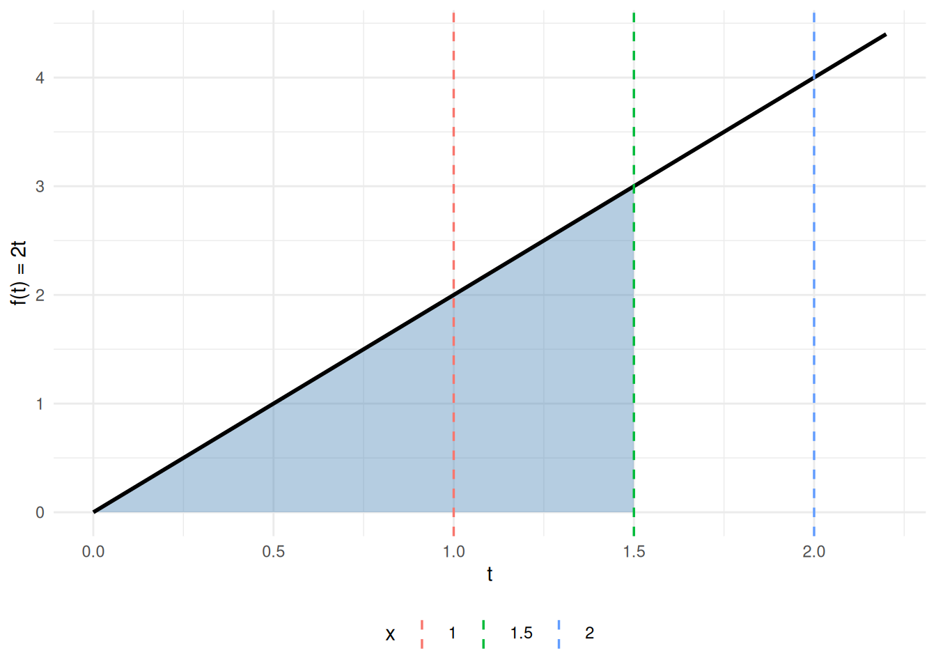
Show R code
slope_df <- tibble::tibble(
  x = x_marks,
  Fx = x_marks^2,
  slope = 2 * x_marks
)

ggplot2::ggplot() +
  ggplot2::geom_function(fun = \(x) x^2, xlim = c(0, 2.2), linewidth = 1) +
  ggplot2::geom_point(
    data = slope_df,
    ggplot2::aes(x = x, y = Fx, color = factor(x)),
    size = 3
  ) +
  ggplot2::geom_segment(
    data = slope_df,
    ggplot2::aes(
      x = x - 0.3, xend = x + 0.3,
      y = Fx - 0.3 * slope, yend = Fx + 0.3 * slope,
      color = factor(x)
    ),
    linewidth = 0.8
  ) +
  ggplot2::labs(x = "x", y = expression(F(x) == x^2), color = "x") +
  ggplot2::theme_minimal() +
  ggplot2::theme(legend.position = "bottom")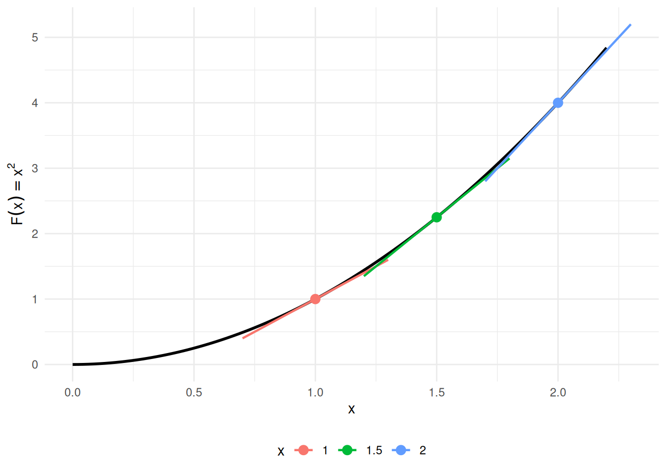
Left: \(f(t) = 2t\); the shaded area
\[ \begin{aligned} \int_0^{1.5} 2t\,dt &= F(1.5) \\ &= 2.25; \end{aligned} \]
ExmExample 23 (CDF and PDF of the exponential distribution)
Example 23 (CDF and PDF of the exponential distribution) In what follows, \(f\) denotes the PDF and \(F\) the CDF — the same letters as the antiderivative pair in Definition 1, because the FTC will show \(F\) is exactly an antiderivative of \(f\).
Let \(T\) be a random variable with the exponential distribution with rate \({\lambda}> 0\). Its probability density function (PDF) is [12, Sec. II], p. 295, “Survival and Hazard Functions for Selected Distributions”:
\[f(t) = {\lambda}\text{e}^{-{\lambda}t}, \quad t \ge 0\]
FTC Part 2 gives the cumulative distribution function (CDF), \(F(t) = P(T \le t)\), from the PDF. Apply the \(\text{e}^{cx}\) rule from Theorem 1 with \(c = -{\lambda}\) to antidifferentiate the integrand:
\[ \begin{aligned} F(t) &= \int_0^t {\lambda}\text{e}^{-{\lambda}u}\,du && \text{(the CDF integrates the PDF)} \\ &= \mathopen{}\left[{\lambda}\cdot\frac{1}{-{\lambda}}\text{e}^{-{\lambda}u}\right]\mathclose{}_{u=0}^{u=t} && \text{(FTC Part 2, with the } \text{e}^{cx} \text{ rule)} \\ &= \mathopen{}\left[(-1)\text{e}^{-{\lambda}u}\right]\mathclose{}_{u=0}^{u=t} && \text{(} {\lambda}/ (-{\lambda}) = -1 \text{)} \\ &= \mathopen{}\left[-\text{e}^{-{\lambda}u}\right]\mathclose{}_{u=0}^{u=t} && \text{(multiply by } -1 \text{)} \\ &= -\text{e}^{-{\lambda}t} - \mathopen{}\left(-\text{e}^{0}\right)\mathclose{} && \text{(evaluate at the limits)} \\ &= -\text{e}^{-{\lambda}t} - (-1) && \text{(} \text{e}^{0} = 1 \text{)} \\ &= 1 - \text{e}^{-{\lambda}t} && \text{(rearrange)} \end{aligned} \]
FTC Part 1 recovers the PDF from the CDF:
\[ \begin{aligned} \frac{\partial}{\partial t} F(t) &= \frac{\partial}{\partial t}\mathopen{}\left(1 - \text{e}^{-{\lambda}t}\right)\mathclose{} && \text{(substitute } F \text{)} \\ &= \frac{\partial}{\partial t} 1 - \frac{\partial}{\partial t} \text{e}^{-{\lambda}t} && \text{(derivative of a difference)} \\ &= 0 - \frac{\partial}{\partial t} \text{e}^{-{\lambda}t} && \text{(constant rule)} \\ &= 0 - \text{e}^{-{\lambda}t} \cdot\frac{\partial}{\partial t}(-{\lambda}t) && \text{(chain rule, with inner function } -{\lambda}t \text{)} \\ &= 0 - \text{e}^{-{\lambda}t} \cdot(-{\lambda}) && \text{(constant multiple rule)} \\ &= {\lambda}\text{e}^{-{\lambda}t} && \text{(simplify)} \\ &= f(t) && \text{(definition of } f \text{)} \end{aligned} \]
For a concrete instance: with \({\lambda}= 1\), the probability that \(T \le 2\) is:
\[ \begin{aligned} F(2) &= 1 - \text{e}^{-1 \cdot 2} \\ &= 1 - \text{e}^{-2} \\ &\approx 1 - 0.135 \\ &= 0.865 \end{aligned} \]
See Figure 5.
Show R code
ggplot2::ggplot() +
  ggplot2::geom_area(
    data = tibble::tibble(t = seq(0, t_focus, length.out = 300)),
    ggplot2::aes(x = t, y = lambda * exp(-lambda * t)),
    fill = "steelblue", alpha = 0.4
  ) +
  ggplot2::geom_function(
    fun = \(t) lambda * exp(-lambda * t),
    xlim = c(0, t_max), linewidth = 1
  ) +
  ggplot2::labs(x = "t", y = "f(t)") +
  ggplot2::theme_minimal()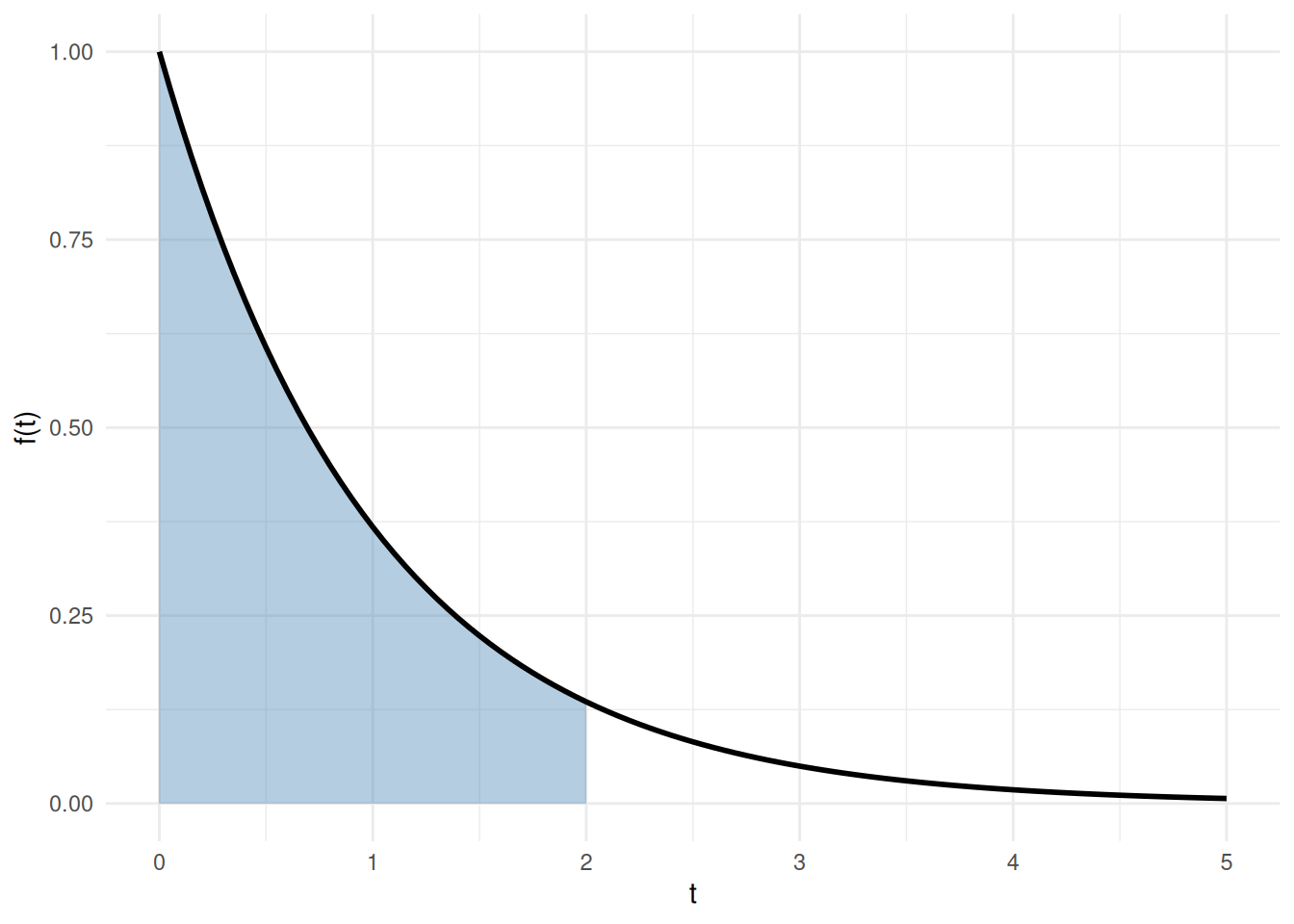
Show R code
ggplot2::ggplot() +
  ggplot2::geom_function(
    fun = \(t) 1 - exp(-lambda * t),
    xlim = c(0, t_max), linewidth = 1
  ) +
  ggplot2::geom_point(
    ggplot2::aes(x = t_focus, y = F_at_focus),
    size = 3, color = "steelblue"
  ) +
  ggplot2::geom_segment(
    ggplot2::aes(x = t_focus, xend = t_focus, y = 0, yend = F_at_focus),
    linetype = "dashed", color = "steelblue"
  ) +
  ggplot2::geom_segment(
    ggplot2::aes(x = 0, xend = t_focus, y = F_at_focus, yend = F_at_focus),
    linetype = "dashed", color = "steelblue"
  ) +
  ggplot2::labs(x = "t", y = "F(t)") +
  ggplot2::theme_minimal()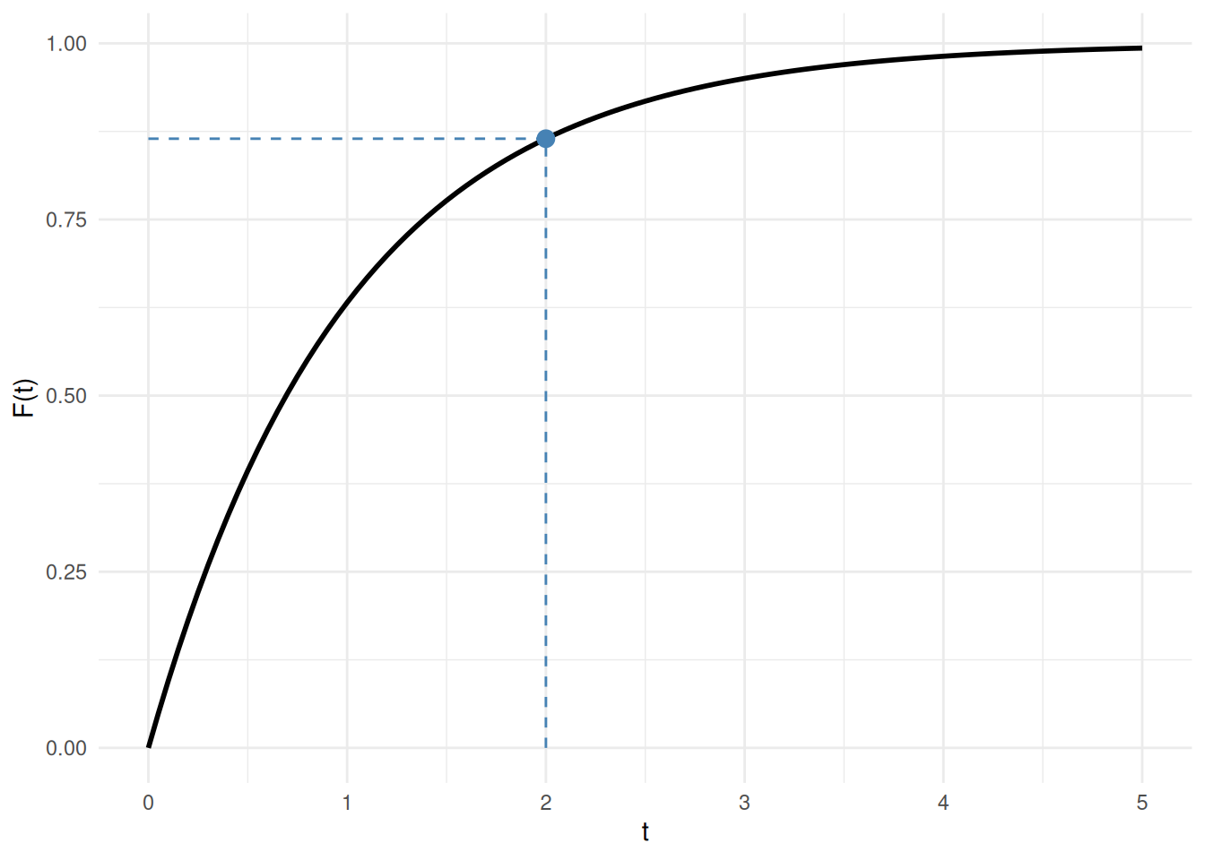
ExrExercise 10 (Improper Gaussian-kernel integral)
Exercise 10 (Improper Gaussian-kernel integral) Adapted from Miller [11], Question 1.1.39.
Evaluate the improper integral:
\[\int_0^\infty x{\operatorname{exp}\mathopen{}\left\{-\frac{x^2}{4}\right\}\mathclose{}}\,dx\]
ExrExercise 11 (Convolution of two uniform densities)
Exercise 11 (Convolution of two uniform densities) Adapted from Miller [11], Question 1.1.41.
Let \(f(x) = \mathbb{1}_{[0, 1]}(x)\) be the indicator of the unit interval:
\[f(x) = \begin{cases} 1 & \text{if } x \in [0, 1] \\ 0 & \text{otherwise} \end{cases}\]
Evaluate the convolution:
\[(f * f)(x) = \int_{-\infty}^\infty f(t)f(x - t)\,dt\]
for all \(x \in \mathbb{R}\).
LemTheorem 7 (Convolution of two uniform densities)
Theorem 7 (Convolution of two uniform densities) Let \(f(x) = \mathbb{1}_{[0, 1]}(x)\) be the indicator of the unit interval. Then for every \(x \in \mathbb{R}\),
\[ (f * f)(x) = \int_{-\infty}^\infty f(t)f(x - t)\,dt = \begin{cases} x & \text{if } 0 \le x \le 1 \\ 2 - x & \text{if } 1 < x \le 2 \\ 0 & \text{otherwise.} \end{cases} \]
ProofProof
Proof. This is the solution to Exercise 11, worked in Solution 11.
The integrand \(f(t)f(x - t)\) equals \(1\) when both \(t \in [0, 1]\) and \(x - t \in [0, 1]\), and \(0\) otherwise. The second condition is \(x - 1 \le t \le x\), so the integrand is \(1\) exactly on the overlap \([\max(0, x - 1), \min(1, x)]\), and the integral is the length of that overlap.
- If \(x < 0\) or \(x > 2\), the overlap is empty, so \((f * f)(x) = 0\).
- If \(0 \le x \le 1\), the overlap is \([0, x]\), so \((f * f)(x) = \int_0^x 1\,dt = x\).
- If \(1 < x \le 2\), the overlap is \([x - 1, 1]\), so \((f * f)(x) = \int_{x-1}^1 1\,dt = 2 - x\).
TipVideos
Jon Krohn’s “Calculus for Machine Learning” YouTube playlist has videos on evaluating definite integrals:
References
[1]
Wikipedia contributors, “Antiderivative — Wikipedia, the free encyclopedia.” 2026. Available: https://en.wikipedia.org/wiki/Antiderivative
[2]
R. Larson and B. H. Edwards, Calculus, 11th ed. Boston, MA: Cengage Learning, 2018. Available: https://www.cengage.com/c/calculus-11e-larson/
[3]
Wikipedia contributors, “Continuous function — Wikipedia, the free encyclopedia.” 2026. Available: https://en.wikipedia.org/wiki/Continuous_function
[4]
Wikipedia contributors, “Classification of discontinuities — Wikipedia, the free encyclopedia.” 2026. Available: https://en.wikipedia.org/wiki/Classification_of_discontinuities
[5]
Wikipedia contributors, “Partition of an interval — Wikipedia, the free encyclopedia.” 2026. Available: https://en.wikipedia.org/wiki/Partition_of_an_interval
[6]
Wikipedia contributors, “Riemann sum — Wikipedia, the free encyclopedia.” 2026. Available: https://en.wikipedia.org/wiki/Riemann_sum
[7]
Wikipedia contributors, “Riemann integral — Wikipedia, the free encyclopedia.” 2026. Available: https://en.wikipedia.org/wiki/Riemann_integral
[8]
W. Rudin, Principles of mathematical analysis, 3rd ed. in International series in pure and applied mathematics. New York: McGraw-Hill, 1976.
[9]
Wikipedia contributors, “Fundamental theorem of calculus — Wikipedia, the free encyclopedia.” 2026. Available: https://en.wikipedia.org/wiki/Fundamental_theorem_of_calculus
[10]
A. D. Banner, The calculus lifesaver : All the tools you need to excel at calculus. in A princeton lifesaver study guide. Princeton, New Jersey: Princeton University Press, 2007. Available: https://press.princeton.edu/books/paperback/9780691130880/the-calculus-lifesaver
[11]
S. J. Miller, The probability lifesaver: Calculus review problems. 2016. Available: https://web.williams.edu/Mathematics/sjmiller/public_html/probabilitylifesaver/index.htm#:~:text=http%3A//web.williams.edu/Mathematics/sjmiller/public_html/probabilitylifesaver/supplementalchap_calcreview.pdf
[12]
D. G. Kleinbaum and M. Klein, Survival analysis: A self-learning text, 3rd ed. Springer, 2012. doi: 10.1007/978-1-4419-6646-9.