Model Selection

Published

Last modified: 2026-10-25

Show code

# The Python chunks on this page import numpy and pandas; reticulate provisions them.
# The Julia chunks run through JuliaCall.
reticulate::py_require(c("numpy", "pandas", "scipy"))

Source

Adapted from Kameron Decker Harris’ 2022 weekly notes.

1 Hyperparameters

A First Model and Generalization introduced the training, validation and test split. It noted that cross-validation (CV) is the alternative when we cannot afford a dedicated validation set. This chapter covers that alternative, and how to tune without overfitting. Choosing among candidates with a validation set or with cross-validation is model selection [1]. These notes say validation set throughout; some sources call the same thing a development set or dev set, and the names are interchangeable.

A hyperparameter is a parameter that controls the structure of the model. We choose it, rather than learning it from the data. Three examples follow, one we have met and two still ahead:

\(\regpar\) — ridge and lasso, in Regularization
\(K\) — the number of neighbors in K-nearest neighbors, in Non-Parametric Models
\(\bandwidth\) — the kernel bandwidth, in Non-Parametric Models: \(k(r) \propto \expf{\dfrac{-r^2}{2\bandwidth^2}}\) for a distance \(r\)

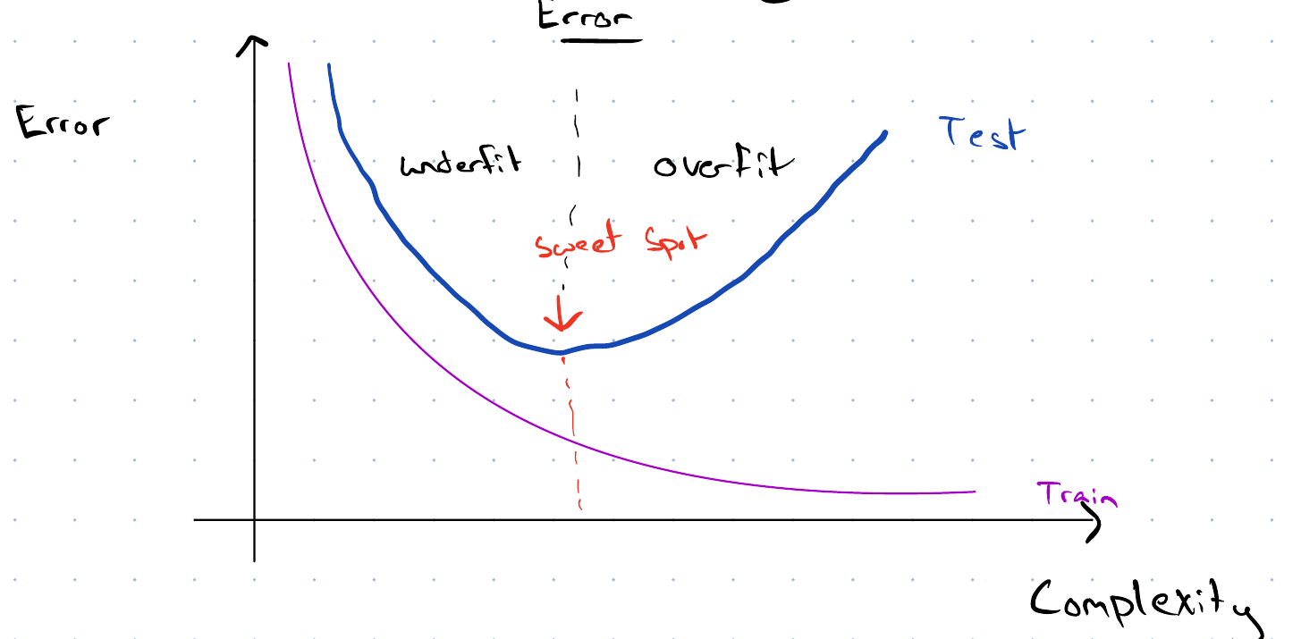
Complexity grows with the number of parameters, and with \(\dfrac{1}{\regpar}\) for a penalized model.

Watch

Hastie and Tibshirani choose a tuning parameter by cross-validation, from 1:54 [2], video 6.8.

Watch

Hutchinson covers train, dev and test sets, cross-validation and model selection, Generalization, part 2 (11 min) [3]. The video site requires a login, which enrolled students find in the syllabus.

2 Training risk cannot choose the model

The empirical risk on the training set cannot choose between a model and a larger one that contains it. That is why we need held-out data.

Theorem 1 (A larger model family never has a larger minimum empirical risk)

Theorem 1 (A larger model family never has a larger minimum empirical risk) Let \(\predfam_1 \subseteq \predfam_2\) be two prediction function families, and let \(\trainset\) be a training set. For any loss, the smallest empirical risk over \(\predfam_2\) is at most the smallest over \(\predfam_1\):

\[ \min_{h \in \predfam_2} \empriskf{h; \trainset} \le \min_{h \in \predfam_1} \empriskf{h; \trainset} . \tag{1}\]

The minima are assumed to exist.

Proof

Proof. Every \(h \in \predfam_1\) is also in \(\predfam_2\), so the minimum over \(\predfam_2\) ranges over every model the minimum over \(\predfam_1\) does, and possibly more.

Example 1 (Adding predictors to a linear model)

Example 1 (Adding predictors to a linear model) Let \(\predfam_1\) be the linear models that use \(p\) predictors, \(\predfnf{\vx} = \dprod{\vx}{\vbeta}\), and let \(\predfam_2\) be the linear models that use those \(p\) predictors and \(q\) more. Setting the \(q\) new coefficients to \(0\) turns any model in \(\predfam_2\) into one in \(\predfam_1\), and every model in \(\predfam_1\) arises this way, so \(\predfam_1 \subseteq \predfam_2\). By Theorem 1, the larger model’s lowest training risk is no higher, whether the loss is squared error, as in least squares, or log loss, as in logistic regression.

Example 2 (Pure-noise predictors lower the training error)

Example 2 (Pure-noise predictors lower the training error) The Auto data give the fuel economy (mpg), horsepower and weight of 392 cars [4, Sec. 5.3]. Fit mpg on horsepower and weight, then add predictors that are pure noise, drawn independently of mpg. Fit each model on half of the cars and score it on the other half.

auto_np <- read.csv("data/auto.csv")

# Alternate rows between the training half and the test half,
# so the split does not depend on a random draw.
is_train_np <- seq_len(nrow(auto_np)) %% 2 == 1

# Draw 30 noise columns once. Using the first k of them gives models that are nested
# by construction, which is what the theorem needs.
set.seed(1)
max_noise_np <- 30
noise_np <- as.data.frame(
  matrix(rnorm(nrow(auto_np) * max_noise_np), ncol = max_noise_np)
)
data_np <- cbind(auto_np[, c("mpg", "horsepower", "weight")], noise_np)

# For each k, fit by least squares on the training half
# (columns 1 to 3 are mpg, horsepower and weight, then the first k noise columns).
# The sample root mean squared error (sRMSE) is the square root of the mean squared error,
# so it is in miles per gallon. The test interval is a 95% t interval for the mean squared error
# on the test half, with its endpoints square-rooted.
rmse_np <- function(k) {
  fit <- lm(mpg ~ ., data = data_np[is_train_np, 1:(3 + k)])
  sq_err <- function(rows) (data_np$mpg[rows] - predict(fit, newdata = data_np[rows, ]))^2
  sq_test <- sq_err(!is_train_np)
  half <- qt(0.975, df = length(sq_test) - 1) * sd(sq_test) / sqrt(length(sq_test))
  c(
    train = sqrt(mean(sq_err(is_train_np))),
    test = sqrt(mean(sq_test)),
    test_lower = sqrt(max(mean(sq_test) - half, 0)),
    test_upper = sqrt(mean(sq_test) + half)
  )
}
ks_np <- 0:max_noise_np
errors_np <- t(sapply(ks_np, rmse_np))
cbind(noise_predictors = ks_np, round(errors_np, 2))[ks_np %in% c(0, 1, 2, 5, 10, 20, 30), ]

     noise_predictors train test test_lower test_upper
[1,]                0  4.38 4.07       3.55       4.53
[2,]                1  4.38 4.07       3.55       4.53
[3,]                2  4.38 4.06       3.54       4.52
[4,]                5  4.36 4.09       3.57       4.54
[5,]               10  4.26 4.17       3.69       4.61
[6,]               20  4.20 4.22       3.76       4.64
[7,]               30  4.18 4.20       3.74       4.62

The table reports the sRMSE, the square root of the mean squared error, so it is in the units of mpg (why we report sRMSE). The training sRMSE does not rise at any of the 30 steps (checked in code, with a tolerance for rounding: TRUE), and it falls from 4.38 to 4.18 mpg. The test sRMSE is higher at the end, 4.20 mpg (95% confidence interval [3.74, 4.62]) against 4.07 mpg ([3.55, 4.53]) with no noise predictors, and it rises at 16 of the 30 steps and falls at the rest. Each test interval is the \(t\) interval for the mean of the 196 test cars’ squared errors, with its endpoints square-rooted. It reflects which test cars were drawn, not which training cars or which noise columns, and both models score the same cars, so the two intervals are not independent. The two intervals overlap heavily, so this one split does not show that the test error rose; the theorem says only that the training error cannot rise. The training sRMSE has no interval, because it describes the cars the model was fit to and is not an estimate of its error on new cars. The new predictors carry no information about mpg, so the fit uses them only to bend toward the noise in the training half.

Remark 1 (Training risk cannot choose between nested models)

Remark 1 (Training risk cannot choose between nested models). By Theorem 1, the training risk ranks nested models by size alone: the largest model always wins or ties, whether or not its extra terms help, as Example 2 shows. Choosing among models therefore needs an estimate of the risk on new data, which is what held-out data and cross-validation supply, or a penalty on size, as Regularization does for the coefficients.

The theorem is about the minimum over each family, for the data the model was fit to. It does not say the larger model’s risk on new data is lower, and the held-out error can end higher, as Example 2 shows.

3 Simple cross-validation

The simplest split is one training set and one test set.

3.1 Assumptions and problems

We assume all data points are independent and identically distributed (IID). A single split has three problems:

The split shrinks the training set.
A random draw picks the validation and test sets.
The resulting error estimate can have high variance.

Watch

Hastie and Tibshirani describe the validation-set approach, from 8:11, and its drawbacks, from 13:14 [2], video 5.1.

Watch

Abu-Mostafa covers model selection with a validation set in his lecture on validation, from 30:47 [5], Lecture 13.

Watch

The CS229 lecture covers data splits, models and cross-validation [6], Lecture 8.

Watch

Lall compares validation approaches in his EE104 lecture on validation, from 14:20 [7], Lecture 4.

4 K-fold cross-validation

Here \(K\) is the number of folds. It has nothing to do with the \(K\) in K-nearest neighbors, listed in Section 1. Both names are standard, so we reuse the letter.

We divide the data into \(K\) blocks. Here \(K=4\):

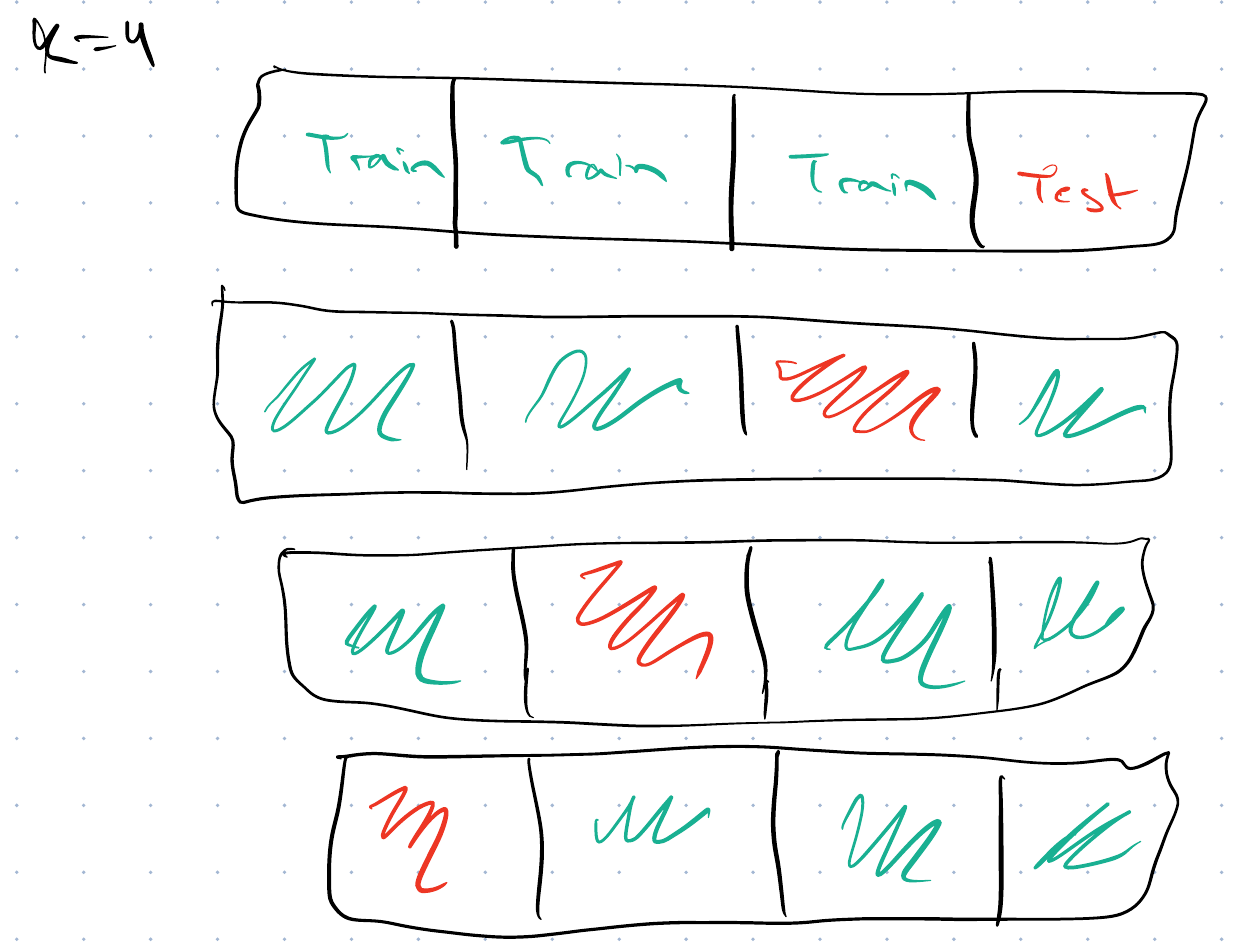
Train blocks and test block rotate across the \(K=4\) folds, and we average the errors, which estimates the risk of the fitted model:

\(\dfrac{1}{K}\sum\limits_{i=1}^{K} \text{error}_i\)

Averaging lowers the variance of the error estimate.

Pros: lower variance

Cons: we fit \(K\) models, which is costly. A small \(K\) might not be reliable.

4.1 Leave-one-out cross-validation

The extreme case is \(K = n\): each fold holds out a single data point.

Watch

Abu-Mostafa explains leave-one-out cross-validation, from 49:03 [5], Lecture 13.

Watch

Hastie and Tibshirani go through \(K\)-fold cross-validation in detail, from 0:55 [2], video 5.2.

Watch

Starmer explains \(K\)-fold cross-validation [8].

Watch

Abu-Mostafa explains \(K\)-fold cross-validation, from 1:06:25 [5], Lecture 13.

Watch

Lall covers cross-validation in his EE104 lecture on validation, from 36:24 [7], Lecture 4.

Read

GeeksforGeeks explains cross-validation [9], including \(K\)-fold and leave-one-out.

Read

The University of Washington’s CSE 446 slides cover train-test splits and cross-validation [10], Lecture 5.

4.2 Choosing the number of folds

The number of folds \(k\) trades the bias of the estimate against its variance. Common choices are \(k = 5\) and \(k = 10\) [11, Sec. 5.1.4], [12, Sec. 7.10]. The statistics notes give a short version. The divs below define the variance of the estimate, then give the bias and the variance side of the trade.

Definition 1 (Variance of the cross-validation estimate)

Definition 1 (Variance of the cross-validation estimate) The variance of the cross-validation estimate is the variance of the \(k\)-fold cross-validation estimate \(\hR_{k\text{-fold}}\) over training sets \(\trainset\) of the same size:

\[ \Var{\hR_{k\text{-fold}}} = \Expfc{\trainset}{\sqf{\hR_{k\text{-fold}} - \Expfc{\trainset}{\hR_{k\text{-fold}}}}} . \tag{2}\]

In words, it is the expected squared distance of the estimate from its own mean over training sets. It says how far the estimate moves when the data are redrawn. It is not the variance of a prediction, which says how far the prediction of one fitted model moves.

Example 3 (How much the cross-validation estimate moves with the data)

Example 3 (How much the cross-validation estimate moves with the data) The Auto data give the fuel economy (mpg) and horsepower of 392 cars [4, Sec. 5.3]. Treat the cars as a population. Draw 40 of them at random as a training set, fit a quadratic regression of mpg on horsepower, and estimate its risk by \(k\)-fold cross-validation with squared error. Then draw a new training set and repeat, 500 times in all. The variance of the estimate is the variance of those 500 estimates.

Python
R

import numpy as np
import pandas as pd

auto_cv_py = pd.read_csv("data/auto.csv")
# Horsepower in hundreds, so the squared term stays on a scale the fit handles well.
hp_cv_py = auto_cv_py["horsepower"].to_numpy(dtype=float) / 100
mpg_cv_py = auto_cv_py["mpg"].to_numpy(dtype=float)
n_train_cv_py = 40
n_rep_cv_py = 500
ks_cv_py = [2, 5, 10, n_train_cv_py]

def mse_cv_py(fit_idx, new_idx):
    # Fit the quadratic to the cars in fit_idx, and score it on the cars in new_idx.
    coef = np.polyfit(hp_cv_py[fit_idx], mpg_cv_py[fit_idx], 2)
    return np.mean((mpg_cv_py[new_idx] - np.polyval(coef, hp_cv_py[new_idx])) ** 2)

rng_cv_py = np.random.default_rng(1)
# One row per training set and one column per fold, for each number of folds k.
fold_err_cv_py = {k: np.empty((n_rep_cv_py, k)) for k in ks_cv_py}
# The risk of the model fitted to the whole training set, estimated on the other cars.
test_cv_py = np.empty(n_rep_cv_py)
for b in range(n_rep_cv_py):
    train = rng_cv_py.choice(len(mpg_cv_py), n_train_cv_py, replace=False)
    new = np.setdiff1d(np.arange(len(mpg_cv_py)), train)
    for k in ks_cv_py:
        fold = rng_cv_py.permutation(np.arange(n_train_cv_py) % k)
        for j in range(k):
            fold_err_cv_py[k][b, j] = mse_cv_py(train[fold != j], train[fold == j])
    test_cv_py[b] = mse_cv_py(train, new)

# The folds have equal sizes, so the estimate is the mean of the fold errors.
est_cv_py = {k: fold_err_cv_py[k].mean(axis=1) for k in ks_cv_py}
var_cv_py = np.array([est_cv_py[k].var(ddof=1) for k in ks_cv_py])
# A 95% interval for a variance, from the normal approximation to the sample variance.
half_cv_py = 1.96 * np.sqrt(2 / (n_rep_cv_py - 1))
print(pd.DataFrame({
    "k": ks_cv_py,
    "variance": var_cv_py.round(1),
    "lower": (var_cv_py * (1 - half_cv_py)).round(1),
    "upper": (var_cv_py * (1 + half_cv_py)).round(1),
}))

    k  variance  lower  upper
0   2     126.6  110.9  142.3
1   5      44.2   38.7   49.6
2  10      39.2   34.4   44.1
3  40      36.7   32.1   41.2

auto_cv <- read.csv("data/auto.csv")
# Horsepower in hundreds, so the squared term stays on a scale the fit handles well.
auto_cv$hp <- auto_cv$horsepower / 100
ks_cv <- c(2, 5, 10, n_train_cv)

mse_cv <- function(d_fit, d_new) {
  # Fit the quadratic to the cars in d_fit, and score it on the cars in d_new.
  fit <- lm(mpg ~ hp + I(hp^2), data = d_fit)
  mean((d_new$mpg - predict(fit, d_new))^2)
}

set.seed(1)
sim_cv <- lapply(seq_len(n_rep_cv), function(b) {
  train <- sample(nrow(auto_cv), n_train_cv)
  d_train <- auto_cv[train, ]
  list(
    # The error in each fold, for each number of folds k.
    fold_err = lapply(ks_cv, function(k) {
      fold <- sample(rep_len(seq_len(k), n_train_cv))
      sapply(seq_len(k), function(j) mse_cv(d_train[fold != j, ], d_train[fold == j, ]))
    }),
    # The risk of the model fitted to the whole training set, estimated on the other cars.
    test = mse_cv(d_train, auto_cv[-train, ])
  )
})

# One row per training set and one column per fold, for each number of folds k.
fold_err_cv <- lapply(seq_along(ks_cv), function(m) t(sapply(sim_cv, function(s) s$fold_err[[m]])))
# The folds have equal sizes, so the estimate is the mean of the fold errors.
est_cv <- sapply(fold_err_cv, rowMeans)
test_cv <- sapply(sim_cv, `[[`, "test")

var_cv <- apply(est_cv, 2, var)
# A 95% interval for a variance, from the normal approximation to the sample variance.
half_cv <- 1.96 * sqrt(2 / (n_rep_cv - 1))
data.frame(
  k = ks_cv,
  variance = round(var_cv, 1),
  lower = round(var_cv * (1 - half_cv), 1),
  upper = round(var_cv * (1 + half_cv), 1)
)

The two tabs draw different random training sets, so their numbers differ by Monte Carlo error. The text quotes the R tab. The intervals treat the estimates as roughly normal, which is only a rough guide with two folds. With \(k = 5\) folds, the estimate has variance 41.8 (95% interval 36.6 to 47.0), so its standard deviation is 6.5. That is how far the 5-fold estimate typically sits from its mean, because the training set is redrawn, even though every estimate scores a model fitted to the same kind of data.

Remark 2 (Fewer folds make the estimate too pessimistic)

Remark 2 (Fewer folds make the estimate too pessimistic). Each of the \(k\) fits in \(k\)-fold cross-validation uses a fraction \((k - 1)/k\) of the data. The estimate therefore scores models fitted to fewer observations than the model we will actually use. A model fitted to less data usually has a larger risk, so the estimate tends to overshoot the risk of the model fitted to all of the data. In other words, the estimate has a positive bias as an estimator of that risk.

The bias shrinks as \(k\) grows. Leave-one-out cross-validation fits each model to \(n - 1\) of the \(n\) observations, so it has the smallest bias of the choices of \(k\) [11, Sec. 5.1.4], [12, Sec. 7.10].

Example 4 (The estimate overshoots most with two folds)

Example 4 (The estimate overshoots most with two folds) Continue Example 3 with the same 500 training sets of 40 cars. For each training set, take the risk of the quadratic fitted to all of its cars, estimated as the mean squared error on the other 352 cars. Subtract that risk from the cross-validation estimate, and average the differences over training sets. The average difference is an estimate of the bias.

Python
R

rows_bias_py = []
for k in ks_cv_py:
    diff = est_cv_py[k] - test_cv_py
    se = diff.std(ddof=1) / np.sqrt(n_rep_cv_py)
    # A 95% interval for the bias, from the normal approximation to the mean of the differences.
    rows_bias_py.append((k, diff.mean(), diff.mean() - 1.96 * se, diff.mean() + 1.96 * se))
print(pd.DataFrame(rows_bias_py, columns=["k", "bias", "lower", "upper"]).round(2))

    k  bias  lower  upper
0   2  3.26   2.22   4.31
1   5  0.52  -0.14   1.19
2  10  0.12  -0.52   0.76
3  40 -0.09  -0.71   0.54

bias_cv <- t(sapply(seq_along(ks_cv), function(m) {
  diff <- est_cv[, m] - test_cv
  se <- sd(diff) / sqrt(n_rep_cv)
  # A 95% interval for the bias, from the normal approximation to the mean of the differences.
  c(k = ks_cv[m], bias = mean(diff), lower = mean(diff) - 1.96 * se, upper = mean(diff) + 1.96 * se)
}))
round(as.data.frame(bias_cv), 2)

With \(k = 2\) folds, each model sees only 20 cars, and the estimate overshoots the risk by 3.83 (95% interval 2.52 to 5.14). With \(k = 5\) the overshoot falls to 0.50, with \(k = 10\) to 0.15, and with \(k = n\) to -0.03. The intervals for \(k = 5\), \(k = 10\) and \(k = n\) all include zero, so these data cannot tell their biases from none.

Remark 3 (Why leave-one-out may have a higher variance (a heuristic))

Remark 3 (Why leave-one-out may have a higher variance (a heuristic)). One reason to suspect that the variance of the cross-validation estimate grows with \(k\) is a heuristic about the correlation of fold errors. A heuristic is not a theorem.

Let:

\(\hR_{I_j}\) be the error in fold \(j\): the mean loss over the observations in fold \(I_j\) of the model fitted to the other folds;
\(\varpar\) be the variance of a fold error over training sets;
\(\bar{\corpar}\) be the average, over two different folds, of the correlation of their errors over training sets.

Assume:

the \(k\) folds have equal sizes, so \(\hR_{k\text{-fold}}\) is the mean of the \(k\) fold errors;
every fold error has the same variance \(\varpar\).

The variance of a mean of \(k\) terms is the sum of their \(k\) variances and \(k(k - 1)\) covariances, divided by \(k^2\):

\[ \Var{\hR_{k\text{-fold}}} = \frac{1}{k^2} \paren{k \varpar + k(k - 1) \bar{\corpar} \varpar} = \frac{\varpar}{k} \paren{1 + (k - 1) \bar{\corpar}} . \tag{3}\]

In words: if the fold errors were uncorrelated (\(\bar{\corpar} = 0\)), averaging them would divide their variance by \(k\). If they were perfectly correlated (\(\bar{\corpar} = 1\)), averaging would not reduce the variance at all.

The heuristic is about \(\bar{\corpar}\). In leave-one-out cross-validation, any two of the \(n\) training sets share \(n - 2\) observations, so the \(n\) fitted models are nearly identical. Their errors may then be strongly correlated, and the average would barely be less variable than one error [12, Sec. 7.10]. For smaller \(k\), the training sets overlap less, so \(\bar{\corpar}\) may be smaller.

The argument is only a heuristic for two reasons. First, \(\varpar\) and \(\bar{\corpar}\) both depend on \(k\), because the fold size changes with \(k\). Second, how correlated the errors are depends on how much the fitted model changes when one observation changes. No estimator of the variance of \(k\)-fold cross-validation is unbiased in general [13], so \(\bar{\corpar}\) is hard to check from a single data set.

Together with the bias of small \(k\), this is the usual reason to choose \(k = 5\) or \(k = 10\): the estimates are neither strongly biased nor, in practice, very variable [11, Sec. 5.1.4], [12, Sec. 7.10].

Example 5 (The correlation of fold errors on the Auto data)

Example 5 (The correlation of fold errors on the Auto data) Continue Example 3 with the same 500 training sets of 40 cars. For each number of folds \(k\), compute the average variance \(\varpar\) of a fold error, the average correlation \(\bar{\corpar}\) between the errors of two folds, and the right side of Equation 3. Compare that to the variance of the estimate itself:

Python
R

rows_var_py = []
for k in ks_cv_py:
    fold_err = fold_err_cv_py[k]
    cors = np.corrcoef(fold_err, rowvar=False)
    sigma2 = fold_err.var(axis=0, ddof=1).mean()
    # The mean of the off-diagonal correlations: remove the k ones on the diagonal.
    rho_bar = (cors.sum() - k) / (k * (k - 1))
    rows_var_py.append((k, est_cv_py[k].var(ddof=1), sigma2, rho_bar,
                        sigma2 / k * (1 + (k - 1) * rho_bar)))
print(pd.DataFrame(rows_var_py, columns=["k", "variance", "sigma2", "rho_bar", "formula"]).round(3))

    k  variance    sigma2  rho_bar  formula
0   2   126.619   208.841    0.214  126.764
1   5    44.157   213.152    0.009   44.166
2  10    39.235   396.870   -0.002   38.796
3  40    36.691  1492.856   -0.001   36.495

var_rows_cv <- t(sapply(seq_along(ks_cv), function(m) {
  k <- ks_cv[m]
  fold_err <- fold_err_cv[[m]]
  sigma2 <- mean(apply(fold_err, 2, var))
  # The mean of the off-diagonal correlations: remove the k ones on the diagonal.
  rho_bar <- (sum(cor(fold_err)) - k) / (k * (k - 1))
  c(k = k, variance = var(est_cv[, m]), sigma2 = sigma2, rho_bar = rho_bar,
    formula = sigma2 / k * (1 + (k - 1) * rho_bar))
}))
round(as.data.frame(var_rows_cv), 3)

The right side of Equation 3 closely matches the simulated variance in every row. It is not exact, because the fold errors do not have exactly equal variances. With \(k = 2\) folds, the two fold errors have correlation 0.13, and the estimate has the largest variance, 212. With \(k = 5\), \(k = 10\) and \(k = n\) the average correlation is 0.01, 0.00 and 0.00, essentially zero. The estimate’s variance is then 42, 36 and 35, and the intervals of Example 3 overlap. So here leave-one-out is no more variable than \(k = 5\) or \(k = 10\). A quadratic least-squares fit is stable: one removed car barely moves it, and the fold errors differ mainly because the folds contain different cars. The heuristic’s worry applies to fitting methods whose predictions change more when one observation changes, and these data do not show it for this one.

5 Cross-validation versus random resampling

With \(K = 4\):

4-fold cross-validation
Average the test errors

vs.

Randomly sample 25% four times

5.1 Is it the same?

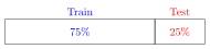
No. Random sampling means the second scenario might not test on 100% of the data. It may also resample points from the test set.

Watch

Hastie and Tibshirani describe the bootstrap, which also resamples the data [2], video 5.4.

Read

GeeksforGeeks explains the bootstrap [14].

6 Cross-validation on real data

Exercise 1 (Choosing a polynomial degree for fuel economy)

Exercise 1 (Choosing a polynomial degree for fuel economy) The Auto data give the fuel economy (mpg) and engine horsepower of 392 cars [4, Sec. 5.3].

For each degree from 1 to 8, fit a polynomial regression of mpg on horsepower. Estimate the test sRMSE of each degree with 10-fold cross-validation.

Solution 1

Solution 1.

Python
R

import numpy as np
import pandas as pd
from scipy import stats

auto_py = pd.read_csv("data/auto.csv")
x = auto_py["horsepower"].to_numpy(dtype=float)
y = auto_py["mpg"].to_numpy(dtype=float)
n_py = len(y)
K = 10
rng = np.random.default_rng(1)
fold_py = rng.permutation(np.arange(n_py) % K)

def sq_err_cv(d):
    # Each car's squared error comes from the fit that left its fold out.
    out = np.empty(n_py)
    for k in range(K):
        train, test = fold_py != k, fold_py == k
        poly = np.polynomial.Polynomial.fit(x[train], y[train], d)
        out[test] = (y[test] - poly(x[test])) ** 2
    return out

sq_py = {d: sq_err_cv(d) for d in range(1, 9)}
cv_rmse_py = pd.Series({d: np.sqrt(sq.mean()) for d, sq in sq_py.items()}, name="cv_rmse")
print(cv_rmse_py.round(2))

1    4.93
2    4.38
3    4.39
4    4.40
5    4.34
6    4.34
7    4.32
8    4.33
Name: cv_rmse, dtype: float64

auto <- read.csv("data/auto.csv")
n <- nrow(auto)
degrees <- 1:8
K <- 10

set.seed(1)
fold <- sample(rep(seq_len(K), length.out = n))

# Each car's squared error comes from the fit that left its fold out.
sq_err_cv <- sapply(degrees, function(d) {
  out <- numeric(n)
  for (k in seq_len(K)) {
    fit <- lm(mpg ~ poly(horsepower, d), data = dplyr::filter(auto, fold != k))
    pred <- predict(fit, dplyr::filter(auto, fold == k))
    out[fold == k] <- (auto$mpg[fold == k] - pred)^2
  }
  out
})
cv_mse <- colMeans(sq_err_cv)
cv_df <- tibble::tibble(degree = degrees, cv_rmse = sqrt(cv_mse))
dplyr::mutate(cv_df, cv_rmse = round(cv_rmse, 2))

The two languages assign the cars to folds at random in different ways, so their estimates differ slightly. The numbers below are from the R fold assignment.

The sample root mean squared error (sRMSE) is the square root of the sample mean squared error, so it is in the units of mpg (why we report sRMSE).

Exercise 2 (Choosing a polynomial degree for fuel economy (part 2))

Exercise 2 (Choosing a polynomial degree for fuel economy (part 2)) Use the setup of Exercise 1.

Give a 95% confidence interval for each estimate.

Solution 2

Solution 2.

Python
R

def rmse_ci(sq):
    # A 95% t interval for the mean squared error, with its endpoints square-rooted.
    half = stats.t.ppf(0.975, df=len(sq) - 1) * sq.std(ddof=1) / np.sqrt(len(sq))
    return np.sqrt(sq.mean()), np.sqrt(max(sq.mean() - half, 0)), np.sqrt(sq.mean() + half)

rows_py = [(d, *rmse_ci(sq)) for d, sq in sq_py.items()]
print(pd.DataFrame(rows_py, columns=["degree", "cv_rmse", "lower", "upper"]).round(2))

   degree  cv_rmse  lower  upper
0       1     4.93   4.54   5.29
1       2     4.38   3.96   4.76
2       3     4.39   3.96   4.78
3       4     4.40   3.97   4.78
4       5     4.34   3.92   4.73
5       6     4.34   3.91   4.72
6       7     4.32   3.89   4.71
7       8     4.33   3.90   4.72

# A 95% t interval for the mean squared error, with its endpoints square-rooted.
half <- qt(0.975, df = n - 1) * apply(sq_err_cv, 2, sd) / sqrt(n)
cv_df <- dplyr::mutate(
  cv_df,
  lower = sqrt(pmax(cv_mse - half, 0)),
  upper = sqrt(cv_mse + half)
)
dplyr::mutate(cv_df, dplyr::across(-degree, \(v) round(v, 2)))

Each interval is the \(t\) interval for the mean of the 392 cross-validated squared errors, with its endpoints square-rooted. It is approximate, because the ten fits share most of their training cars, so the errors are not independent, and the interval tends to be too narrow [15]. Every degree scores the same cars, so the intervals are not independent and say little about which degree is better.

Exercise 3 (Choosing a polynomial degree for fuel economy (part 3))

Exercise 3 (Choosing a polynomial degree for fuel economy (part 3)) Use the setup of Exercise 1.

Which degree has the lowest estimate?

Solution 3

Solution 3.

best <- degrees[which.min(cv_df$cv_rmse)]

The lowest estimate is for degree 7, with a cross-validated sRMSE of 4.32 mpg (95% confidence interval [3.89, 4.70]). Figure 1 plots all eight estimates with their intervals.

Show code

library(ggplot2)
ggplot(cv_df, aes(degree, cv_rmse)) +
  geom_line() +
  geom_pointrange(aes(ymin = lower, ymax = upper)) +
  geom_point(data = cv_df[cv_df$degree == best, ], shape = 1, size = 5) +
  scale_x_continuous(breaks = degrees) +
  labs(x = "polynomial degree", y = "10-fold CV estimate of test sRMSE (mpg)")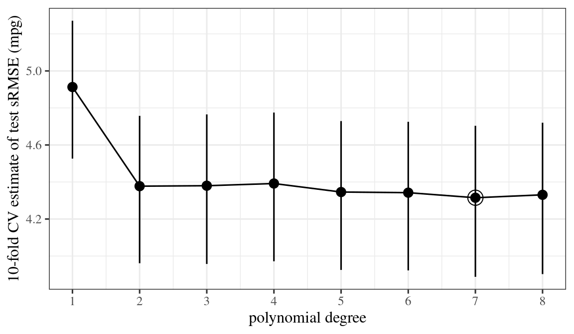

A ggplot2 chart with polynomial degree from 1 to 8 on the horizontal axis and estimated test root mean squared error in miles per gallon on the vertical axis. Each degree has a point with a vertical interval. The error is highest for degree 1, drops sharply at degree 2, and changes little for higher degrees, where the intervals overlap heavily. An open circle marks the lowest point, at one of the highest degrees. — Figure 1: Ten-fold cross-validation estimate of the test sample root mean squared error (sRMSE) for polynomial regressions of mpg on horsepower, by degree, with 95% confidence intervals. The open circle marks the degree with the lowest estimate. The intervals are approximate and probably too narrow.

Exercise 4 (Choosing a polynomial degree for fuel economy (part 4))

Exercise 4 (Choosing a polynomial degree for fuel economy (part 4)) Use the setup of Exercise 1.

Is the lowest estimate much lower than the one for the straight line?

Solution 4

Solution 4. The straight line has 4.91 ([4.53, 5.27]), so degree 2 already lowers the estimate by 0.54 mpg, which is 11% of the straight line’s value. Going from degree 2 to degree 7 lowers it by only 0.06 mpg more, well inside the interval for degree 2, 3.96 to 4.76. A simpler model whose estimate is this close to the lowest one is often the better choice.

Read

The resampling lab in An Introduction to Statistical Learning: With Applications in Python (ISLP) repeats this analysis in Python [4, Sec. 5.3], ISLP_labs, Ch05.

7 Multiple hyperparameters

Hyperparameters multiply. With

\[\regpar \in \{10^{-3}, 10^{-2}, 10^{-1}, 10^{0}, 10^{1}\} \quad \textcolor{blue}{5}\] \[\text{(Degree)} \quad d \in \{2, 3, 4\} \quad \textcolor{blue}{3}\]

there are \(5 \cdot 3 = 15\) hyperparameter combinations to search.

7.1 Searching the grid

The search is simple. We fit every combination on each of the \(K\) training blocks. We score it on the held-out block, average over the blocks, and take the combination with the smallest sample average. The code in the Python, R and Julia tabs does exactly that. The data come from a cubic. So the right answer is known: \(d = 3\), with as little regularization as the noise allows.

The code never penalizes the intercept. Shrinking it would pull the fitted surface toward zero rather than toward the mean. That depends on the units of the response, not on model complexity. The code also assigns the folds once, outside the grid loop. Every combination is therefore scored on the same partition. Re-drawing the folds per combination would add variation that has nothing to do with the hyperparameters. The comparison is between combinations.

import numpy as np

def design(x, d):
    return np.column_stack([x ** k for k in range(d + 1)])

def ridge(X, y, lam):
    P = np.eye(X.shape[1]); P[0, 0] = 0          # never penalize the intercept
    return np.linalg.solve(X.T @ X + lam * P, X.T @ y)

def cv_error(x, y, d, lam, K, folds):
    errs = []
    for k in range(K):
        tr, te = folds != k, folds == k
        beta = ridge(design(x[tr], d), y[tr], lam)
        errs.append(np.mean((y[te] - design(x[te], d) @ beta) ** 2))
    return np.mean(errs)                          # (1/K) sum of fold errors

rng = np.random.default_rng(0)
truth = lambda x: 1 - 2 * x + 0.5 * x**2 + 0.8 * x**3
n, K = 60, 4
x = rng.uniform(-2, 2, n)
y = truth(x) + rng.normal(scale=1.0, size=n)
folds = rng.permutation(np.arange(n) % K)         # K blocks, shuffled

grid = [(d, lam) for d in (2, 3, 4) for lam in (1e-3, 1e-2, 1e-1, 1e0, 1e1)]
scores = {(d, lam): cv_error(x, y, d, lam, K, folds) for d, lam in grid}
print("combinations searched:", len(scores))

combinations searched: 15

for d in (2, 3, 4):
    print(d, [round(float(scores[(d, lam)]), 3) for lam in (1e-3, 1e-2, 1e-1, 1e0, 1e1)])

2 [2.221, 2.221, 2.22, 2.215, 2.175]
3 [1.177, 1.177, 1.176, 1.178, 1.405]
4 [1.188, 1.188, 1.186, 1.177, 1.388]

best = min(scores, key=scores.get)
print("best (degree, lambda):", best, "cv error:", round(scores[best], 3))

best (degree, lambda): (3, 0.1) cv error: 1.176

# The winner's own CV score is not an estimate of its error.
xt = rng.uniform(-2, 2, 10_000)
yt = truth(xt) + rng.normal(scale=1.0, size=10_000)
beta = ridge(design(x, best[0]), y, best[1])
print("fresh test error:", round(np.mean((yt - design(xt, best[0]) @ beta) ** 2), 3))

fresh test error: 1.029

design <- function(x, d) outer(x, 0:d, `^`)

ridge <- function(X, y, lam) {
  P <- diag(ncol(X)); P[1, 1] <- 0            # never penalize the intercept
  solve(t(X) %*% X + lam * P, t(X) %*% y)
}

cv_error <- function(x, y, d, lam, K, folds) {
  errs <- numeric(K)
  for (k in seq_len(K)) {
    tr <- folds != k
    beta <- ridge(design(x[tr], d), y[tr], lam)
    errs[k] <- mean((y[!tr] - design(x[!tr], d) %*% beta)^2)
  }
  mean(errs)                                   # (1/K) sum of fold errors
}

set.seed(0)
truth <- function(x) 1 - 2 * x + 0.5 * x^2 + 0.8 * x^3
n <- 60; K <- 4
x <- runif(n, -2, 2)
y <- truth(x) + rnorm(n)
folds <- sample(rep_len(1:K, n))                # K blocks, shuffled

grid <- expand.grid(lam = c(1e-3, 1e-2, 1e-1, 1e0, 1e1), d = 2:4)
grid <- dplyr::mutate(grid,
                       cv = mapply(function(d, lam) cv_error(x, y, d, lam, K, folds), grid$d, grid$lam))
cat("combinations searched:", nrow(grid), "\n")

combinations searched: 15

for (d in 2:4) cat(d, round(grid$cv[grid$d == d], 3), "\n")

2 2.251 2.251 2.249 2.237 2.151 
3 0.844 0.844 0.847 0.89 1.364 
4 0.85 0.851 0.857 0.93 1.602

best <- dplyr::slice(grid, which.min(cv))
cat("best (degree, lambda):", best$d, best$lam, "cv error:", round(best$cv, 3), "\n")

best (degree, lambda): 3 0.001 cv error: 0.844

# The winner's own CV score is not an estimate of its error.
xt <- runif(10000, -2, 2); yt <- truth(xt) + rnorm(10000)
beta <- ridge(design(x, best$d), y, best$lam)
cat("fresh test error:", round(mean((yt - design(xt, best$d) %*% beta)^2), 3), "\n")

fresh test error: 1.045

using Random, Statistics, LinearAlgebra

design(x, d) = [xi^k for xi in x, k in 0:d];

function ridge(X, y, lam)
    P = Matrix{Float64}(I, size(X, 2), size(X, 2))
    P[1, 1] = 0                                  # never penalize the intercept
    return (X'X + lam * P) \ (X'y)
end;

function cv_error(x, y, d, lam, K, folds)
    errs = Float64[]
    for k in 1:K
        tr = folds .!= k
        beta = ridge(design(x[tr], d), y[tr], lam)
        push!(errs, mean((y[.!tr] - design(x[.!tr], d) * beta) .^ 2))
    end
    return mean(errs)                            # (1/K) sum of fold errors
end;

Random.seed!(0);
truth(x) = 1 - 2x + 0.5x^2 + 0.8x^3;
n, K = 60, 4;
x = 4 .* rand(n) .- 2;
y = truth.(x) .+ randn(n);
# K blocks, shuffled
folds = shuffle([mod1(i, K) for i in 1:n]);

grid = [(d, lam) for d in 2:4 for lam in (1e-3, 1e-2, 1e-1, 1e0, 1e1)];
scores = Dict(g => cv_error(x, y, g[1], g[2], K, folds) for g in grid);
println("combinations searched: ", length(scores))

combinations searched: 15


for d in 2:4
    println(d, " ", [round(scores[(d, lam)], digits = 3)
                     for lam in (1e-3, 1e-2, 1e-1, 1e0, 1e1)])
end

2 [2.575, 2.575, 2.574, 2.562, 2.479]
3 [1.222, 1.222, 1.221, 1.23, 1.62]
4 [1.233, 1.233, 1.236, 1.29, 1.889]


# Minimise over the ordered grid, not over the Dict: a Dict iterates in
# hash order, so argmin(scores) would break a tie unpredictably.
best = argmin(g -> scores[g], grid);
println("best (degree, lambda): ", best, " cv error: ", round(scores[best], digits = 3))

best (degree, lambda): (3, 0.1) cv error: 1.221


# The winner's own CV score is not an estimate of its error.
xt = 4 .* rand(10_000) .- 2;
yt = truth.(xt) .+ randn(10_000);
beta = ridge(design(x, best[1]), y, best[2]);
println("fresh test error: ",
        round(mean((yt - design(xt, best[1]) * beta) .^ 2), digits = 3))

fresh test error: 1.034

Show code

# What each tab printed, stored as values for the table in the next section.
tab_d = best[0]
tab_cv, tab_test = float(scores[best]), float(np.mean((yt - design(xt, best[0]) @ beta) ** 2))

Show code

tab_r <- c(d = best$d, cv = best$cv, test = mean((yt - design(xt, best$d) %*% beta)^2))

Show code

tab_d = best[1];
tab_cv, tab_test = scores[best], mean((yt - design(xt, best[1]) * beta) .^ 2);

Show code

f3 <- function(v) sprintf("%.3f", v)
f4 <- function(v) sprintf("%.4f", v)
jl <- function(expr) JuliaCall::julia_eval(expr)
tab_cv <- c(reticulate::py$tab_cv, tab_r[["cv"]], jl("tab_cv"))
tab_test <- c(reticulate::py$tab_test, tab_r[["test"]], jl("tab_test"))
n_high <- sum(tab_cv > tab_test)
count_word <- function(k) c("none", "one", "two", "all three")[k + 1]

Every tab rejects \(d = 2\) by a wide margin, and all three are nearly flat in \(\regpar\) until it reaches \(10\), at which point the penalty adds more bias than the variance it removes. The winning degree is \(3\) in the Python tab, \(3\) in R and \(3\) in Julia, against a true degree of \(3\): \(d = 3\) and \(d = 4\) score close together in every tab, so a different draw of the data can tip the choice between them. The degree matters here and the penalty barely does. Yet a grid search reports a winner whether or not the axes it searched were the ones that mattered.

Read

GeeksforGeeks explains hyperparameter tuning [16], including grid search.

7.2 The winning score is not an error estimate

Each tab also fits the winner on all \(n\) points and scores it on fresh data. Compare that number with the CV score that selected it:

	CV score of the winner	fresh test error
Python	1.176	1.029
R	0.844	1.045
Julia	1.221	1.034

The CV score is too high in two of the three tabs and too low in one. A single sample therefore cannot answer the question. Two effects act in opposite directions. Only repeating the whole experiment separates them.

We repeat the entire procedure 400 times, with fresh data, fresh folds and a fresh grid search. The noise variance stays fixed at \(1\). Averaging over the replications gives:

Show code

# The listing at the end of this section, generalized to every grid and seed
# the prose quotes. Takes about 40 seconds. Each replication draws its data once
# and scores every candidate on it, so every grid sees identical data, as the
# listing's own grid does. Solving for all the lambdas of one degree at once
# gives the listing's CV scores for its own grid.
import numpy as np

def design(x, d):
    return np.column_stack([x ** k for k in range(d + 1)])

truth = lambda x: 1 - 2 * x + 0.5 * x**2 + 0.8 * x**3
n, K, R = 60, 4, 400
five = [1e-3, 1e-2, 1e-1, 1e0, 1e1]
fine = list(np.logspace(-3, 1, 15))
grids = {
    "15": [(d, lam) for d in (2, 3, 4) for lam in five],
    "45": [(d, lam) for d in (2, 3, 4) for lam in fine],
    "75": [(d, lam) for d in (2, 3, 4, 5, 6) for lam in fine],
}
for lam in five:
    grids["lam%g" % lam] = [(d, lam) for d in (2, 3, 4)]

def replicate(seed, which):
    cands = sorted({c for g in which for c in grids[g]})
    rng = np.random.default_rng(seed)
    xt = rng.uniform(-2, 2, 200_000)
    yt = truth(xt) + rng.normal(scale=1.0, size=200_000)
    Xt = {d: design(xt, d) for d, _ in cands}
    out = {g: dict(cv=[], part=[], full=[], win=[]) for g in which}
    s45 = []
    for _ in range(R):
        x = rng.uniform(-2, 2, n)
        y = truth(x) + rng.normal(scale=1.0, size=n)
        folds = rng.permutation(np.arange(n) % K)
        s, fit0 = {}, {}
        for d in sorted({d for d, _ in cands}):
            L = np.array([lam for dd, lam in cands if dd == d])
            X = design(x, d)
            P = np.eye(d + 1); P[0, 0] = 0
            errs = np.zeros(len(L))
            for k in range(K):
                tr, te = folds != k, folds == k
                A = X[tr].T @ X[tr] + L[:, None, None] * P
                b = np.broadcast_to(X[tr].T @ y[tr], (len(L), d + 1))[..., None]
                betas = np.linalg.solve(A, b)[..., 0]
                if k == 0:
                    fit0.update({(d, lam): bt for lam, bt in zip(L, betas)})
                errs += np.mean((y[te][:, None] - X[te] @ betas.T) ** 2, axis=0)
            s.update({(d, lam): e for lam, e in zip(L, errs / K)})
        true_err = {}
        for g in which:
            w = min(grids[g], key=lambda c: s[c])
            if w not in true_err:
                d, lam = w
                P = np.eye(d + 1); P[0, 0] = 0
                X = design(x, d)
                full = np.linalg.solve(X.T @ X + lam * P, X.T @ y)
                true_err[w] = (np.mean((yt - Xt[d] @ fit0[w]) ** 2),
                               np.mean((yt - Xt[d] @ full) ** 2))
            out[g]["cv"].append(s[w])
            out[g]["win"].append(w)
            out[g]["part"].append(true_err[w][0])
            out[g]["full"].append(true_err[w][1])
        if "45" in which:
            s45.append([[s[(d, lam)] for lam in fine] for d in (2, 3, 4)])
    res = {g: {k: np.mean(v) for k, v in o.items() if k != "win"} for g, o in out.items()}
    for r in res.values():
        r["bias"] = r["part"] - r["cv"]       # selection bias
        r["size"] = r["part"] - r["full"]     # training-size effect
    return res, out, np.array(s45)

rep_res, rep_out, s45 = replicate(1, list(grids))
new_wins = sum(lam not in five for _, lam in rep_out["45"]["win"])
adj_lam = np.mean(np.abs(np.diff(s45, axis=2)))
adj_deg = np.mean(np.abs(np.diff(s45, axis=1)))
by_seed = [rep_res["15"]] + [replicate(seed, ["15"])[0]["15"] for seed in (0, 2, 3, 4)]
seed_cv = np.array([r["cv"] for r in by_seed])
seed_bias = np.array([r["bias"] for r in by_seed])
seed_size = np.array([r["size"] for r in by_seed])
seed_net = seed_bias - seed_size

Show code

rr <- reticulate::py$rep_res
g15 <- rr[["15"]]
g45 <- rr[["45"]]
g75 <- rr[["75"]]
lam_bias <- function(lam) rr[[paste0("lam", lam)]]$bias
pm <- function(v) sprintf("%.4f \\pm %.4f", mean(v), sd(v))
drop45 <- g15$cv - g45$cv
drop75 <- g45$cv - g75$cv

quantity	value
CV score of the selected combination	1.070
its true error, fit on \(\tfrac{K-1}{K}\) of the data	1.113
its true error, refit on all \(n\)	1.086

The first gap is selection bias, also called the winner’s curse. Each of the 15 scores is a noisy estimate. Taking the smallest of 15 preferentially picks a combination whose noise happened to be low. So the winning score understates even its own model’s error, by \(0.0422\) here. (The table’s rounded rows differ by \(0.043\). Subtracting two three-decimal figures leaves at most three decimals of signal. The result can be off by one in the last decimal. That matters when we compare selection bias across grids, because the whole question is how far these move. The figures quoted here are all differences of the unrounded sample means.)

Selection bias grows with the number of distinct, competitive candidates rather than with the raw count. We re-run the replication over other grids, with the same \(n\), the same \(K\) and the same 400 replications. Every run uses seed \(1\), so every grid sees identical data. The results are:

grid	candidates	selection bias
\(d \in \{2,3,4\}\), \(\regpar = 10^{-2}\) alone	3	\(0.0377\)
\(d \in \{2,3,4\}\), the five \(\regpar\)s used here	15	\(0.0422\)
\(d \in \{2,3,4\}\), `np.logspace(-3, 1, 15)`	45	\(0.0434\)
\(d \in \{2,\dots,6\}\), the same fifteen \(\regpar\)s	75	\(0.0700\)

Tripling the count from 15 to 45 barely moves it. Adding \(d = 5\) and \(d = 6\) to reach seventy-five raises it from \(0.0434\) to \(0.0700\), a factor of \(1.62\). Both steps add thirty candidates, so the count does not separate them. Nor does the finer grid go unused. That grid keeps only three of the original five \(\regpar\)s, and its twelve new values win \(258\) of the \(400\) replications. They win, but they add few new independent candidates. Across that 45-candidate grid, two \(\regpar\)-adjacent candidates differ in CV score by \(0.0159\) on average, where two degree-adjacent candidates at the same \(\regpar\) differ by \(0.5207\). The finer grid therefore gains very little from noise the five \(\regpar\)s had not already exposed. It lowers the sample mean winning score by \(0.0009\), against \(0.0075\) for the two added degrees.

A falling winning score is most of the first step and less than a third of the second. Selection bias is the winner’s true error minus its CV score. So it can widen from either end. These two steps widen it from different ends. From 15 candidates to 45 the bias grows by \(0.0012\), and the falling score supplies \(0.0009\) of that. From 45 to 75 it grows by \(0.0267\), of which the falling score supplies \(0.0075\); the remaining \(0.0192\) is the winner’s own true error going up. Degrees \(5\) and \(6\) do not only give the search more chances to draw a low score. They change which model it chooses, for the worse.

The first row depends on which single \(\regpar\) we fix, because that is a choice rather than a constant. At \(\regpar = 10^{-3}\) the same three degrees give \(0.0376\) and at \(10^{-1}\), \(0.0371\); at \(\regpar = 1\), \(0.0348\); at \(\regpar = 10\), \(0.0447\). That is higher than the fifteen-candidate grid, on only three candidates. That last row lies outside the argument rather than contradicting it. At \(\regpar = 10\) every fit is badly over-regularized, with a CV score of \(1.356\) against \(1.070\). So the comparison is among three bad candidates rather than competitive ones.

The second gap runs the other way. A CV score measures a model fit on \(\tfrac{K-1}{K}\) of the data. The model we deploy is fit on all of it, so it is slightly better, by \(0.0262\) here. So a small \(K\) is pessimistic. Leave-one-out cross-validation avoids that.

Overall, the CV score of the winner is optimistic by \(0.0159\) in this run. That remainder is the difference of two close numbers, so it is the least stable quantity here. We repeat the whole 400-replication experiment under seeds \(0\) through \(4\). We change only default_rng(1). Selection bias comes out at \(0.0394 \pm 0.0051\) and the training-size effect at \(0.0265 \pm 0.0025\), each clearly positive or clearly negative. Their difference comes out at \(0.0129 \pm 0.0073\), and one of the five runs lands at \(0.0003\). Here \(\pm\) is the sample standard deviation across the five runs. We carry more digits than elsewhere because this paragraph is about how far they move.

So the two biases nearly cancel. Four hundred replications do not settle whether the remainder is optimism or pessimism. One run settles it even less. We cannot control either bias. The practical consequence is the same either way. A score used to choose a model cannot also be used to report it. Keep a test set that the search never touched. Alternatively, wrap the whole search in an outer cross-validation loop and report that score. This approach, nested CV, costs another factor of \(K\). Its estimate is not biased by the search.

Listing 1: The replication behind the CV-score and true-error figures

# Takes about 25 seconds. design, ridge and cv_error repeat the Python tab
# of "Searching the grid", because every block here runs on its own. Keep the two copies
# identical: they are the same three functions, not two variants of them.
import numpy as np
from collections import Counter

def design(x, d):
    return np.column_stack([x ** k for k in range(d + 1)])

def ridge(X, y, lam):
    P = np.eye(X.shape[1]); P[0, 0] = 0          # never penalize the intercept
    return np.linalg.solve(X.T @ X + lam * P, X.T @ y)

def cv_error(x, y, d, lam, K, folds):
    errs = []
    for k in range(K):
        tr, te = folds != k, folds == k
        beta = ridge(design(x[tr], d), y[tr], lam)
        errs.append(np.mean((y[te] - design(x[te], d) @ beta) ** 2))
    return np.mean(errs)                          # (1/K) sum of fold errors

truth = lambda x: 1 - 2 * x + 0.5 * x**2 + 0.8 * x**3
grid = [(d, lam) for d in (2, 3, 4) for lam in (1e-3, 1e-2, 1e-1, 1e0, 1e1)]
n, K, R = 60, 4, 400
rng = np.random.default_rng(1)
xt = rng.uniform(-2, 2, 200_000)
yt = truth(xt) + rng.normal(scale=1.0, size=200_000)
test_err = lambda beta, d: np.mean((yt - design(xt, d) @ beta) ** 2)

win_cv, win_test, refit_all, chosen = [], [], [], []
for _ in range(R):
    x = rng.uniform(-2, 2, n)
    y = truth(x) + rng.normal(scale=1.0, size=n)
    folds = rng.permutation(np.arange(n) % K)
    s = {g: cv_error(x, y, g[0], g[1], K, folds) for g in grid}
    b = min(s, key=s.get)
    chosen.append(b)
    win_cv.append(s[b])
    tr = folds != 0                      # all but one fold: (K-1)/K of the data
    win_test.append(test_err(ridge(design(x[tr], b[0]), y[tr], b[1]), b[0]))
    refit_all.append(test_err(ridge(design(x, b[0]), y, b[1]), b[0]))

print(round(np.mean(win_cv), 3), round(np.mean(win_test), 3),
      round(np.mean(refit_all), 3))

1.07 1.113 1.086

print(Counter(d for d, _ in chosen).most_common())

[(3, 297), (4, 103)]

The last line of Listing 1 counts the degrees the search chose. The search found the true degree in 297 of 400 replications and over-fit to \(d = 4\) in the other 103. It never once chose \(d = 2\). Cross-validation is far better at rejecting a model that is too simple than one that is too complex. We can shrink an unnecessary term toward zero, but we cannot create a missing one. So we should extend the grid beyond where we expect the answer to lie.

Watch

Hastie and Tibshirani show cross-validation done the wrong way and the right way [2], video 5.3.

Versions

We rendered this page with NumPy 2.5.3 on Python 3.13.5, R 4.5.3, and Julia 1.12.6. The three tabs disagree on the winning combination and on the sign of the CV-versus-test gap. Each language’s generator produces different data, which explains the disagreement. That disagreement is the point of Section 7.2, not a defect. Every figure here is seeded, so it reproduces exactly on these versions. The sample averages over the replications, however, are seeded Monte Carlo estimates, not constants. The five independent runs under seeds \(0\) through \(4\) spread over \(1.066\) to \(1.083\) on the first row. Treat the third digit as an artifact of the seed.

8 Further reading

James et al. [11], Chapter 5
Hastie et al. [12], Chapter 7
Zhou [17], Resampling Methods — slides on An Introduction to Statistical Learning, Chapter 5, with code in R
Starmer [18], on cross-validation — an illustrated walk-through with little algebra

Watch

The Data Science Learning Community’s book clubs discuss An Introduction to Statistical Learning, Chapter 5, in recorded meetings:

the R book club, in part 1 and part 2 [19];
the Python book club, in one meeting [20].

References

[1]

Wikipedia contributors, “Model selection — Wikipedia, the free encyclopedia.” 2026. Available: https://en.wikipedia.org/wiki/Model_selection

[2]

T. Hastie, R. Tibshirani, and J. Taylor, “Statistical learning with python.” Stanford Online, lecture videos on YouTube, 2023. Available: https://www.youtube.com/playlist?list=PLoROMvodv4rPP6braWoRt5UCXYZ71GZIQ

[3]

B. Hutchinson, “DATA 471/571 (machine learning) and CSCI 481/581 (deep learning) video lectures.” Western Washington University. Accessed: Sep. 28, 2026. [Online]. Available: https://facultyweb.cs.wwu.edu/~hutchib2/video_lectures/data371/

[4]

G. James, D. Witten, T. Hastie, R. Tibshirani, and J. Taylor, An introduction to statistical learning: With applications in Python. Springer, 2023. doi: 10.1007/978-3-031-38747-0.

[5]

Y. S. Abu-Mostafa, “Learning from data: CS 156 lectures.” Caltech, lecture videos on YouTube, 2012. Available: https://www.youtube.com/playlist?list=PLD63A284B7615313A

[6]

A. Ng et al., “CS229: Machine learning, autumn 2018.” Stanford Online, lecture videos on YouTube, 2018. Available: https://www.youtube.com/playlist?list=PLoROMvodv4rMiGQp3WXShtMGgzqpfVfbU

[7]

S. Lall, “EE104: Introduction to machine learning, 2020.” Stanford Online, lecture videos on YouTube, 2020. Available: https://www.youtube.com/playlist?list=PLoROMvodv4rN_Uy7_wmS051_q1d6akXmK

[8]

J. Starmer, “Machine learning fundamentals: Cross validation.” StatQuest, video on YouTube, 2018. Available: https://www.youtube.com/watch?v=fSytzGwwBVw

[9]

GeeksforGeeks, “Cross validation in machine learning.” GeeksforGeeks, tutorial article, 2026. Available: https://www.geeksforgeeks.org/machine-learning/cross-validation-machine-learning/

[10]

N. Jaques, “CSE 446/546: Machine learning, lecture slides.” University of Washington, 2026. Accessed: Oct. 12, 2026. [Online]. Available: https://courses.cs.washington.edu/courses/cse446/26sp/schedule/lectures/

[11]

G. James, D. Witten, T. Hastie, and R. Tibshirani, An introduction to statistical learning with applications in R, 2nd ed. Springer, 2021. Available: https://www.statlearning.com/

[12]

T. Hastie, R. Tibshirani, and J. Friedman, The elements of statistical learning: Data mining, inference, and prediction, 2nd ed. Springer, 2009. Available: https://hastie.su.domains/ElemStatLearn/

[13]

Y. Bengio and Y. Grandvalet, “No unbiased estimator of the variance of K-fold cross-validation,” Journal of Machine Learning Research, vol. 5, pp. 1089–1105, 2004, Available: https://www.jmlr.org/papers/v5/grandvalet04a.html

[14]

GeeksforGeeks, “Bootstrap method.” GeeksforGeeks, tutorial article, 2025. Available: https://www.geeksforgeeks.org/maths/bootstrap-method/

[15]

S. Bates, T. Hastie, and R. Tibshirani, “Cross-validation: What does it estimate and how well does it do it?” Journal of the American Statistical Association, vol. 119, no. 546, pp. 1434–1445, 2024, doi: 10.1080/01621459.2023.2197686.

[16]

GeeksforGeeks, “Hyperparameter tuning.” GeeksforGeeks, tutorial article, 2026. Available: https://www.geeksforgeeks.org/machine-learning/hyperparameter-tuning/

[17]

J. Zhou, “Biostat 212A: Statistical machine learning a, winter 2026.” UCLA, course webpage with lecture slides, 2026. Available: https://ucla-biostat-212a.github.io/2026winter/

[18]

J. Starmer, The StatQuest illustrated guide to machine learning. StatQuest Publications, 2022. Available: https://statquest.org/statquest-store/

[19]

Data Science Learning Community, “Introduction to statistical learning using R (islr06).” Book club meeting recordings on YouTube, 2023. Available: https://www.youtube.com/playlist?list=PL3x6DOfs2NGjlhpKMiWsDcKL2nngwXROq

[20]

Data Science Learning Community, “Introduction to statistical learning using Python (islp03).” Book club meeting recordings on YouTube, 2025. Available: https://www.youtube.com/playlist?list=PL3x6DOfs2NGgbSNh0UG87rrM-z5LiKLZp