A confusion matrix is a matrix \(M \in \reals^{C \times C}\)
\(M_{ij}\) is the number of datapoints in class \(i\) that the model predicts as class \(j\)
Some sources flip the axes (\(M^T\))
Compute them with from sklearn.metrics import confusion_matrix
We can treat this as a detection task for any of the classes. Instead of \(\{dog, cat\}\), we detect dog (\(\modmemf{x} = isDog(x) \in \{T, F\}\)). Write \(\eoutvar_{(i)} = \modmemf{\predvar_{(i)}}\) for the prediction on example \(i\). Then \(M\) has the following form: \[M =
\begin{bmatrix}
T_p & F_n \\
F_p & T_n
\end{bmatrix}\]
Definition 1 (Confusion matrix) For a detection task on \(N\) labelled examples, the confusion matrix counts the examples by true label and predicted label [2]:
The entries are the numbers of true positives \(T_p\) (positives predicted positive), false negatives \(F_n\) (positives predicted negative), false positives \(F_p\) (negatives predicted positive), and true negatives \(T_n\) (negatives predicted negative). The row sums \(T_p + F_n\) and \(F_p + T_n\) are fixed by the data, whatever the rule.
ExrExercise 1 (Count the four ways a detector can be right or wrong)
Exercise 1 (Count the four ways a detector can be right or wrong) In the course overview we wrote a spam rule by hand from five columns of Hastie, Tibshirani and Friedman’s spam data:
if %george\(< 0.6\) and %you\(> 1.5\), then spam; else email.
That is the same 4601 messages, and the data are downloadable: the collection is the Spambase data set of Mark Hopkins, Erik Reeber, George Forman and Jaap Suermondt, at https://archive.ics.uci.edu/dataset/94/spambase. Of the 4601 messages, 1813 are spam and 2788 are email.
Running that rule over all 4601 messages gives these counts:
Table 1: The rule’s predictions against the truth.
Actually spam
Actually email
Predicted spam
1217
726
Predicted email
596
2062
Name each of the four cells: true positive, false positive, false negative, true negative. Take positive to denote “this message is spam”.
\(T_p = 1217\) messages are spam and were called spam. \(F_n = 596\) are spam and were called email — the rule missed them. \(F_p = 726\) are email and were called spam. \(T_n = 2062\) are email and were called email.
The names are worth reading as two words each rather than as four labels. The second word gives what the detector said; the first word gives whether it was right. A false negative is a negative call that was false.
ExrExercise 2 (Count the four ways a detector can be right or wrong (part 2))
Exercise 2 (Count the four ways a detector can be right or wrong (part 2)) Use the setup of Exercise 1.
Which sums must hold among the four cells and the totals?
The row sums of \(M\) are fixed by the data and do not depend on the rule at all. Only the split within each row is the rule’s doing. Remember this: any metric computed down a column mixes the two classes together, and any metric computed along a row does not.
ExrExercise 4 (Count the four ways a detector can be right or wrong (part 4))
Exercise 4 (Count the four ways a detector can be right or wrong (part 4)) Use the setup of Exercise 1.
Two of the four cells are errors. Describe each one in a sentence a user of the mail system would recognize, with no jargon in it.
Solution 4. A false negative is a spam message that arrives in your inbox. A false positive is a real message that arrives in your spam folder.
ExrExercise 5 (Count the four ways a detector can be right or wrong (part 5))
Exercise 5 (Count the four ways a detector can be right or wrong (part 5)) Use the setup of Exercise 1.
One of those two errors is much worse than the other for a mail system. Which, and why? Nothing about the table tells you the answer, so say what does.
Solution 5. The false positive is worse, for almost any mail system. A spam message in the inbox costs a second of attention; a real message in the spam folder may never be read at all, and the sender has no way to know.
Notice that nothing in Table 1 says so. The table counts both errors and weighs neither. The judgment comes from outside the data — from what the system is for, and from who bears the cost of each mistake. This is the reason a single number is never enough on its own, and the reason the rest of the chapter is a list of different numbers rather than a search for the best one.
ExrExercise 6 (Count the four ways a detector can be right or wrong (part 6))
Exercise 6 (Count the four ways a detector can be right or wrong (part 6)) Use the setup of Exercise 1.
A confusion matrix for \(C\) classes is a \(C \times C\) matrix \(M\) with \(M_{ij}\) the number of points whose true class is \(i\) and whose predicted class is \(j\). Write Table 1 in that form, and say which entries are the correct predictions in general.
Solution 6. Classes are “spam” and “email”; take \(i = 1\) for spam and \(i = 2\) for email. Then \(M_{11} = T_p\), \(M_{12} = F_n\), \(M_{21} = F_p\), \(M_{22} = T_n\), which is the matrix in Solution 1. In general the correct predictions are the diagonal entries \(M_{ii}\): true class \(i\), predicted class \(i\). Everything off the diagonal is an error, and its position says which error — \(M_{ij}\) counts class \(i\) mistaken for class \(j\).
ExrExercise 7 (Count the four ways a detector can be right or wrong (part 7))
Exercise 7 (Count the four ways a detector can be right or wrong (part 7)) Use the setup of Exercise 1.
Some textbooks and some software write the transpose of this matrix. How would you tell, from a printed matrix alone, which convention was used?
Solution 7. You can tell from the row and column sums whenever the two classes have different sizes. Here the rows sum to \(1813\) and \(2788\), which are the numbers of spam and email messages; the columns sum to \(1943\) and \(2658\), which are the numbers of messages the rule called spam and email. If you know how many messages of each class the data actually contain, the margin that matches is the one indexed by the true class.
ExrExercise 8 (Count the four ways a detector can be right or wrong (part 8))
Exercise 8 (Count the four ways a detector can be right or wrong (part 8)) Use the setup of Exercise 1.
Give a confusion matrix whose convention you could not tell from the printed matrix alone, as in Exercise 7.
Solution 8. You could not tell if the two margins happened to agree — for instance if the detector called exactly as many messages spam as there are spam messages. A symmetric matrix is the extreme case: it equals its own transpose, so no reading of the margins can separate the conventions. When in doubt, read the documentation of whatever produced the matrix, or feed it a case whose answer you know.
Definition 2 (Accuracy) The accuracy of a classifier on \(N\) examples is the fraction that it classifies correctly [5]. If \(M_{ij}\) is the number of examples in class \(i\) that it predicts as class \(j\), with \(C\) classes,
so the rule labels about 71% of the 4601 messages correctly, and \(Err = 0.2873\).
ExrExercise 10 (Ask what a metric would say about a detector that does nothing (part 2))
Exercise 10 (Ask what a metric would say about a detector that does nothing (part 2)) Use the setup of Exercise 9.
Now consider two detectors that ignore the message entirely: one calls everything spam, the other calls everything email. Give the confusion matrix of each, and compute the accuracy of each.
Solution 12. The rule in general: a detector that always guesses one class gets exactly the frequency of that class, so the best do-nothing detector gets the frequency of the majority class. That number is the baseline any real detector has to beat, and it is a property of the data rather than of the detector.
ExrExercise 13 (Ask what a metric would say about a detector that does nothing (part 5))
Exercise 13 (Ask what a metric would say about a detector that does nothing (part 5)) Use the setup of Exercise 9.
How much accuracy did the hand-written rule gain over the better of the two do-nothing detectors?
Solution 13. \(0.7127 - 0.6060 = 0.1067\). So two hand-picked columns out of 57, with two hand-picked thresholds, gain about eleven percentage points over guessing “email” every time. The rule’s accuracy has a 95% interval of [70.0, 72.6]% and the baseline’s [59.2, 62.0]%, each the proportion plus or minus 1.96 standard errors. They are scored on the same messages, so compare them message by message: the difference in the fraction right is 10.7 percentage points, with a 95% \(t\) interval of [8.8, 12.5], which excludes 0.
ExrExercise 14 (Ask what a metric would say about a detector that does nothing (part 6))
Exercise 14 (Ask what a metric would say about a detector that does nothing (part 6)) Use the setup of Exercise 9.
Solution 14. Whether that is a lot depends on what you were expecting. It is a real improvement, and it is a modest one: a rule that got only these two numbers to look at is doing better than nothing and nowhere near well enough to run a mail system. Both halves of that sentence matter, and quoting \(0.7127\) on its own hides the second.
ExrExercise 15 (Ask what a metric would say about a detector that does nothing (part 7))
Exercise 15 (Ask what a metric would say about a detector that does nothing (part 7)) Use the setup of Exercise 9.
Suppose instead that 50 messages in a million were spam. What accuracy does the “everything is email” detector get?
Solution 16. A detector that has never detected anything reports 99.995% accuracy. The number is not wrong — it correctly answers a question that nobody cares about. Accuracy weighs every message equally, and when almost every message is negative, it is almost entirely a measurement of the negatives.
This is the single most common way a metric misleads, and it has a name: class imbalance. Exercise 59 returns to it once there are metrics that survive it.
ExrExercise 17 (Ask what a metric would say about a detector that does nothing (part 9))
Exercise 17 (Ask what a metric would say about a detector that does nothing (part 9)) Use the setup of Exercise 9.
Prevalence is the fraction of the data that is positive. Express the accuracy of each do-nothing detector in terms of the prevalence \(\prevalence\), and say which one wins as a function of \(\prevalence\).
Calling everything positive wins when \(\prevalence > 1/2\), calling everything negative wins when \(\prevalence < 1/2\), and at \(\prevalence = 1/2\) they tie at \(0.5\). So the do-nothing baseline is \(\max(\prevalence, 1-\prevalence)\), which is never below \(0.5\) and rises toward \(1\) as the classes become more unbalanced. Here
Each of these four rates carries several names, and all of them are still in current use.
This chapter
Also called
Precision
positive predictive value (PPV)
Recall
sensitivity, true positive rate (TPR), hit rate
Specificity
true negative rate (TNR), selectivity
False positive rate (FPR)
false alarm rate, fall-out
The names come from three different fields. Sensitivity, specificity and positive predictive value are the medical and epidemiological names; hit rate and false alarm rate come from signal detection; precision and recall come from information retrieval. A paper reporting sensitivity is reporting recall.
The false positive rate is also written \(1 - \text{specificity}\), which is a formula rather than a further name, and Exercise 18 asks you to compute it for a worked rule.
DefDefinition 4 (Precision (also called positive predictive value))
Definition 4 (Precision (also called positive predictive value)) The precision, also called the positive predictive value (PPV), of a detector is the fraction of its detections that are correct [6]. Write \(P\) for it:
\[
P = \frac{T_p}{T_p + F_p}.
\]
If the detector makes no detections, then \(T_p + F_p = 0\) and the precision is undefined.
DefDefinition 5 (Recall (also called sensitivity or true positive rate))
Definition 5 (Recall (also called sensitivity or true positive rate)) The recall, also called the sensitivity or the true positive rate (TPR), of a detector is the fraction of the positives that it detects [6]. Write \(R\) for it:
\[
R = \frac{T_p}{T_p + F_n}.
\]
If there are no positives, then \(T_p + F_n = 0\) and the recall is undefined.
DefDefinition 6 (Specificity (also called true negative rate))
Definition 6 (Specificity (also called true negative rate)) The specificity, also called the true negative rate (TNR), of a detector is the fraction of the negatives that it correctly leaves undetected [7],
\[
\mathrm{TNR} = \frac{T_n}{F_p + T_n}.
\]
If there are no negatives, then \(F_p + T_n = 0\) and the specificity is undefined.
ExrExercise 18 (Split the errors: precision and recall)
Exercise 18 (Split the errors: precision and recall) Accuracy adds the two kinds of error together. The next two metrics each look at one of them.
So about 63% of the messages the rule sent to the spam folder belonged there, and about 67% of the spam was caught. Treating the messages as a sample, the 95% intervals are [60.5, 64.8]% for precision, from the 1943 flagged messages, and [65.0, 69.3]% for recall, from the 1813 spam messages. Each is the proportion plus or minus 1.96 standard errors, \(\sqrt{\hat p (1 - \hat p) / n}\) with its own \(n\), and it describes which messages happened to be in the data, since the rule was fixed in advance.
ExrExercise 19 (Split the errors: precision and recall (part 2))
Exercise 19 (Split the errors: precision and recall (part 2)) Use the setup of Exercise 18.
Each of the two is a fraction of one margin of the confusion matrix. Which margin is which, and which of the two depends on the number of spam messages in the data?
Solution 19. Precision divides by \(T_p + F_p = 1943\), the number of messages the detector called spam — a column sum, which the detector controls. Recall divides by \(T_p + F_n = 1813\), the number of messages that are spam — a row sum, which is fixed by the data.
So recall has a denominator nobody can change, and precision has one the detector can change by flagging more or fewer messages. That asymmetry makes precision the harder of the two to interpret, so the next exercise sweeps a threshold rather than quoting a single pair.
ExrExercise 20 (Split the errors: precision and recall (part 3))
Exercise 20 (Split the errors: precision and recall (part 3)) Use the setup of Exercise 18.
A detector flags 20 messages, and 15 of them are spam. The data hold 60 spam messages. Compute its precision and recall.
Perfect recall, which is exactly as impressive as it sounds — you can have it at no cost. Its precision is the prevalence, which is the general rule: flag everything and your precision is whatever fraction of the data was positive.
Solution 27. The honest report is “precision undefined; no positive predictions”, not \(0\) and not \(1\). Software will often return \(0\) here, which is a convention rather than a computation — and it is a consequential one, because a metric of \(0\) reads as tested and bad rather than as not tested.
ExrExercise 28 (Split the errors: precision and recall (part 11))
Exercise 28 (Split the errors: precision and recall (part 11)) Use the setup of Exercise 18.
Specificity is \(T_n / (T_n + F_p)\). Compute it for the rule. It looks like a mirror image of precision — say precisely what it measures that precision does not, using the row-and-column observation from Solution 7.
Specificity divides by \(F_p + T_n = 2788\), the number of messages that are email — so, like recall, it is a row and not a column. Precision and specificity both react to false positives, but they normalize by different things: precision asks what fraction of the flags were wrong, and specificity asks what fraction of the real email got flagged.
The difference matters most under imbalance. Flag 726 of 2788 emails and specificity is a moderate \(0.74\); flag 726 of a million emails and specificity is \(0.9993\), while precision is unchanged if the spam count is unchanged. Specificity has the big class in its denominator, so a rare-event problem inflates it.
ExrExercise 29 (Split the errors: precision and recall (part 12))
Exercise 29 (Split the errors: precision and recall (part 12)) Use the setup of Exercise 18.
Recall is also called sensitivity, and \(1 - {}\)specificity is the false positive rate. Give the false positive rate for the rule, and say which of the two classes each of sensitivity and specificity is computed from.
or directly \(726/2788\), with a 95% interval of [24.4, 27.7]% for the false positive rate (the same interval, reflected, for the specificity).
Sensitivity is computed entirely from the positive class: it is the spam row of the matrix. Specificity is computed entirely from the negative class: it is the email row. Neither one can be changed by adding or removing messages of the other class, which makes the pair the natural axes for the ROC curve in Exercise 52.
ExrExercise 30 (Split the errors: precision and recall (part 13))
Exercise 30 (Split the errors: precision and recall (part 13)) Use the setup of Exercise 18.
A colleague reports that their spam detector has 99% precision. Give two questions you would ask before believing the detector is good.
What is the recall?Precision of 99% is trivial to achieve by flagging one message you are certain about and nothing else.
What is the prevalence in the data it was measured on? If the test set was half spam, 99% precision is a real achievement. If it was tuned and measured on the same messages, or if the test set was built by collecting spam until there was a lot of it, the number does not transfer to a real inbox.
A third question: on which messages? A detector measured on last year’s spam is being asked an easier question than the one it will face.
Precision, recall and \(F_\recallweight\) are all defined for a detection task, so for \(C > 2\) we reduce to detection first. The standard reduction is one-vs-rest. We take each class \(c\) in turn, relabel every point as \(c\) or \(\lnot c\), and read the resulting \(2 \times 2\) matrix directly from \(M\),
The diagonal entry counts the true positives. The rest of row \(c\) counts the class-\(c\) points the model mislabeled, and the rest of column \(c\) counts the other points it mislabeled as \(c\).
That leaves \(C\) binary problems and \(C\) values of whichever metric you wanted. Two conventions collapse them to one number. They differ only in when the averaging happens.
Macro-averaging computes the metric per class, then averages: \[P_{macro} = \frac{1}{C}\sumto{c}{C} \frac{T_p^{(c)}}{T_p^{(c)} + F_p^{(c)}},
\qquad
R_{macro} = \frac{1}{C}\sumto{c}{C} \frac{T_p^{(c)}}{T_p^{(c)} + F_n^{(c)}}\] Every class contributes equally, however rare it is.
Micro-averaging pools the counts, then computes the metric once: \[P_{micro} = \frac{\sum_c T_p^{(c)}}{\sum_c T_p^{(c)} + \sum_c F_p^{(c)}},
\qquad
R_{micro} = \frac{\sum_c T_p^{(c)}}{\sum_c T_p^{(c)} + \sum_c F_n^{(c)}}\] Every point contributes equally, so large classes dominate.
When every point gets exactly one predicted label, each mistake is a false positive for exactly one class and a false negative for exactly one other, so \(\sum_c F_p^{(c)} = \sum_c F_n^{(c)}\) and the two micro quantities coincide with each other and with accuracy: \(P_{micro} = R_{micro} = \mathrm{Acc}\).
The same two conventions apply to \(F_\recallweight\), and the order of operations matters more there than it does for \(P\) and \(R\). We compute micro-\(F_1\) from the pooled counts, so it is the \(F_1\) formula applied to \(P_{micro}\) and \(R_{micro}\) — which makes it accuracy again when every point gets exactly one predicted label, since then \(P_{micro} = R_{micro} = \mathrm{Acc}\). Macro-\(F_1\) is the mean of the \(C\) per-class \(F_1\) scores, and that is not the \(F_1\) formula applied to \(P_{macro}\) and \(R_{macro}\): the formula is not linear in \(P\) and \(R\), so averaging before combining and combining before averaging give different numbers.
Discussion: under what class proportions and per-class scores do macro- and micro-averaging agree? What has to be true of the errors for the two to diverge sharply?
Balanced accuracy (higher is better)
\(R_{macro}\) has its own name, balanced accuracy (\(\mathrm{BAcc}\)), because it fixes the most common failure of accuracy: \[\mathrm{BAcc} = \frac{1}{C}\sumto{c}{C} \frac{T_p^{(c)}}{T_p^{(c)} + F_n^{(c)}}\]
Averaging the per-class recalls gives each class equal weight regardless of size, so a model that ignores a rare class scores \(0\) on that class’s term however few points it contains [10]. A classifier guessing uniformly at random scores \(1/C\) whatever the class proportions are, which accuracy does not.
Take \(C = 3\) and \(N = 90\), with \(M_{ij}\) the number of class-\(i\) points predicted as class \(j\) — rows are the true class, columns the prediction:
true class
pred 1
pred 2
pred 3
row total
1
3
7
0
10
2
0
50
0
50
3
0
12
18
30
The diagonal sums to \(71\), so \(\mathrm{Acc} = 71/90 \approx 0.789\), which looks fairly high. The per-class recalls are \(3/10 = 0.3\), \(50/50 = 1.0\) and \(18/30 = 0.6\), giving \(\mathrm{BAcc} = 1.9/3 \approx 0.633\). Class 2 accounts for the whole difference: it holds \(50\) of the \(90\) points and is classified perfectly, so under accuracy it dominates the score, while class 1 — right less than a third of the time — can only ever move the total by \(10\) points.
NoteOther names for \(F_1\), and one number that is not \(F_1\)
Balanced \(F\)-score is a fourth name for \(F_1\), alongside the three the chapter already gives. Image segmentation adds a fifth, the Dice coefficient, usually written as an agreement between two sets rather than as a combination of two rates: \[
\text{Dice} = \frac{2\abs{ A \cap B}}{\abs{ A} +\abs{ B}}.
\] Take \(A\) to be the items the model called positive and \(B\) the items that actually were. Then \(\abs{ A \cap B} = T_p\), \(\abs{ A} = T_p + F_p\), \(\abs{ B} = T_p + F_n\), and the fraction becomes \(2T_p / (2T_p + F_p + F_n)\), to which \(2PR/(P+R)\) reduces. The two are one number under two names, not two measures that happen to agree.
The Jaccard index, also called intersection over union (IoU), looks like a sixth name and is not one: \[
\begin{aligned}
J
&= \frac{\abs{ A \cap B}}{\abs{ A \cup B}} \\
&= \frac{T_p}{T_p + F_p + F_n}.
\end{aligned}
\] Both denominators count each mistake once. They differ in the true positives, which \(J\) counts once and \(F_1\) counts twice. The two always rank a set of models the same way, since \(J = F_1 / (2 - F_1)\) is increasing in \(F_1\), but they are different numbers, and \(J \le F_1\) for every model, with equality only at \(0\) and at \(1\). How far apart they are depends on the value of \(F_1\). The gap \(F_1 - J\) is widest in the middle of the range, reaching \(3 - 2\sqrt 2 \approx 0.17\) at \(F_1 = 2 - \sqrt 2 \approx 0.59\), and closes at both ends. The proportion\(J / F_1 = 1/(2 - F_1)\) behaves differently: it falls steadily as the model gets worse, so a model scoring \(F_1 = 0.99\) reports a Jaccard index \(99\%\) as large, while one scoring \(F_1 = 0.1\) reports one only \(53\%\) as large. Quote whichever you like, and say which one it is.
Definition 7 (F-measure (also called F-score)) For the precision \(P\) and recall \(R\) of a detector (Definition 4, Definition 5) and a weight \(\recallweight > 0\), the F-measure, also called the F-score[11], is
Definition 8 (F1 score) The F1 score of a detector is the F-measure with \(\recallweight = 1\) (Definition 7), the harmonic mean of its precision \(P\) and recall \(R\),
\[
F_1 = \frac{2 P R}{P + R}.
\]
ExrExercise 31 (Combine precision and recall into one number, carefully)
Exercise 31 (Combine precision and recall into one number, carefully) We would like one number, and we have two. The usual way to combine them is the F-measure:
\[F_\recallweight = (1 + \recallweight^2) \frac{P \cdot R}{\recallweight^2 P + R},
\qquad F_1 = 2\frac{P \cdot R}{P + R}.\] Compute \(F_1\) for the rule in Exercise 1.
A detector that flags every single message scores \(F_1 = 0.5653\), and the hand-written rule scores \(0.6480\). The rule is better, and not by as much as one might hope, and \(F_1\) shows this in a way that accuracy did not.
Show code
# No formula gives a simple interval for F1, which is a ratio of counts,# so resample the messages with replacement and recompute F1 each time.set.seed(1)spam_f1_boot<-replicate(1000, {i<-sample(spam_n, replace =TRUE)tp<-sum(spam_data$spam[i]==1&spam_pred_hand[i]==1)fp<-sum(spam_data$spam[i]==0&spam_pred_hand[i]==1)fn<-sum(spam_data$spam[i]==1&spam_pred_hand[i]==0)2*tp/(2*tp+fp+fn)})spam_f1_ci<-quantile(spam_f1_boot, c(0.025, 0.975))
A 95% bootstrap interval for the rule’s \(F_1\) is [0.6308, 0.6663], the middle 95% of 1000 recomputations on messages drawn with replacement. It lies above the \(F_1\) of 0.5653 for flagging everything.
ExrExercise 33 (Combine precision and recall into one number, carefully (part 3))
Exercise 33 (Combine precision and recall into one number, carefully (part 3)) Use the setup of Exercise 31.
Compute \(F_1\) for the do-nothing detector of Exercise 9 that calls every message email.
Solution 34. The precision\(P\) is undefined, so \(F_1\) is undefined too. Even if you substitute \(P = 0\) by convention, \(R = 0\) as well, and the formula gives \(0/0\).
ExrExercise 35 (Combine precision and recall into one number, carefully (part 5))
Exercise 35 (Combine precision and recall into one number, carefully (part 5)) Use the setup of Exercise 31.
Show that \(F_1\) is the harmonic mean of \(P\) and \(R\), that is, \(F_1 = 2 / (1/P + 1/R)\).
Solution 37. The arithmetic mean says “moderate”; \(F_1\) says “this detector is nearly useless”, which is the truth — it flags almost nothing, and is right when it does. The harmonic mean is pulled toward the smaller of its arguments, so a good score on one axis cannot make up for a bad score on the other. That is the whole reason it is the mean used here.
In the extreme case this is clear: if either \(P\) or \(R\) is \(0\), then \(F_1 = 0\), whereas the arithmetic mean would still report half of whatever the other one was.
ExrExercise 38 (Combine precision and recall into one number, carefully (part 8))
Exercise 38 (Combine precision and recall into one number, carefully (part 8)) Use the setup of Exercise 31.
Take the limits \(\recallweight \to 0\) and \(\recallweight \to \infty\) in the formula for \(F_\recallweight\). Which metric does each one recover?
Solution 39. They are backwards. Large \(\recallweight\) favors recall, which is the opposite of what the symbol’s position in the formula suggests at a glance — \(\recallweight^2\) multiplies \(P\) in the denominator, and a bigger denominator term for \(P\) makes \(P\) matter less.
ExrExercise 40 (Combine precision and recall into one number, carefully (part 10))
Exercise 40 (Combine precision and recall into one number, carefully (part 10)) Use the setup of Exercise 31.
State in one sentence what the weight \(\recallweight\) in \(F_\recallweight\) controls.
Solution 40. The rule, in one sentence: \(\recallweight\) is how many times as much you care about recall as about precision. \(F_2\) counts recall twice as heavily; \(F_{0.5}\) counts precision twice as heavily.
ExrExercise 41 (Combine precision and recall into one number, carefully (part 11))
Exercise 41 (Combine precision and recall into one number, carefully (part 11)) Use the setup of Exercise 31.
A medical screening test is followed by a cheap confirmatory test, so a false positive costs a second test and a false negative costs a missed diagnosis. Would you tune \(\recallweight\) above or below 1?
Solution 41. Above 1. A false negative is the expensive error, recall is the metric that counts false negatives, and large \(\recallweight\) favors recall — so \(F_2\) or a similar value. The cheap confirmatory test makes the false positives affordable.
ExrExercise 42 (Combine precision and recall into one number, carefully (part 12))
Exercise 42 (Combine precision and recall into one number, carefully (part 12)) Use the setup of Exercise 31.
\(F_1\) ignores \(T_n\) entirely — it appears nowhere in \(P\) or \(R\). Give a situation where that is exactly what you want, and one where it hides something you need to know.
Solution 42. \(F_1\) ignores the true negatives, so it is unmoved by how many uninteresting things the detector correctly ignored.
You want that when the negatives are arbitrary in number: a web search over ten billion pages that returns ten good results has ten billion true negatives, and any metric containing \(T_n\) would be a measurement of the size of the web rather than of the search. Precision, recall and \(F_1\) all stay the same if you add a billion irrelevant pages, which is the property wanted here.
It hides something when you need to know what fraction of the negatives were harmed. \(F_1\) never divides by the number of emails, so the rule’s \(F_1 = 0.6480\) is unchanged whether its 726 false positives were drawn from the 2788 real emails here or from a million. Those are very different mail systems: in the first, \(726/2788 = 26.04\%\) of your real mail is in the spam folder; in the second, \(0.07\%\) of it is. Specificity and the false positive rate see that difference, because the negative count is in their denominator, and \(F_1\) cannot. When both classes matter, report the confusion matrix, not a summary of it.
If the model outputs \(P(true|x)\), then we can trade off precision against recall by adjusting the threshold, \(\thresh\): \[\modmemf{x} = I(P(true|x) > \thresh)\]
The area under the precision-recall curve (PR AUC) summarizes the curve in a single number
A random scorer’s PR AUC is not \(0.5\); Exercise 59 asks what it is.
ExrExercise 43 (Move the threshold and watch the metrics move)
Exercise 43 (Move the threshold and watch the metrics move) Every metric so far was computed from one confusion matrix, which came from one rule. A model that outputs a probability does not give you one rule — it gives you a family of them, one per threshold:
Solution 44. It has to. Raising \(\thresh\) can only remove messages from the set the model calls spam — a message with \(P(\text{spam} \mid \vx) > \thresh'\) also satisfies \(P > \thresh\) for any \(\thresh < \thresh'\). So \(T_p\) can only fall. Meanwhile \(T_p + F_n = 1813\) is the number of spam messages in the data, which no threshold can change. A quantity that can only fall, divided by a constant, can only fall.
ExrExercise 45 (Move the threshold and watch the metrics move (part 3))
Exercise 45 (Move the threshold and watch the metrics move (part 3)) Use the setup of Exercise 43.
Now describe what happens to precision. It is not monotone. Explain why your proof in Exercise 43 does not apply to precision.
The proof in Solution 43 worked because recall’s denominator was fixed. Precision’s is not: its denominator is \(T_p + F_p\), the number of messages the modelcalled spam, and that shrinks as \(\thresh\) rises too. Both the numerator and the denominator fall, so the ratio can move in either direction.
ExrExercise 46 (Move the threshold and watch the metrics move (part 4))
Exercise 46 (Move the threshold and watch the metrics move (part 4)) Use the setup of Exercise 43.
Give a concrete reason why precision might fall at a high threshold for this particular model, given that it is looking at only two words.
Solution 46. Look at what a high score tells you about this model. With only %george and %you to go on, the score is large when george never appears and you appears very often. The highest-scoring message in the data has \(\texttt{\%you} = 18.75\) and is real email; of the twenty highest-scoring messages, sixteen are real email. Among the top fifty, the spam fraction is \(0.22\) — below the overall prevalence of \(0.3940\), so at the extreme the model is worse than a random guess that says spam with probability equal to the overall spam rate.
Those messages are short personal notes. A model looking at two words cannot tell a chatty email from a sales pitch, and the higher you push \(\thresh\), the more the surviving messages are selected for the one property the model mistakes for spam.
There is a second lesson underneath. %george averages \(1.27\) in email and \(0.00\) in spam, which made it look so useful in the course overview. But \(72.31\%\) of the real emails contain the word george zero times; the average comes from the minority that do, where it averages \(4.57\). A feature can separate the two classes on average and still say nothing about most individual cases.
ExrExercise 47 (Move the threshold and watch the metrics move (part 5))
Exercise 47 (Move the threshold and watch the metrics move (part 5)) Use the setup of Exercise 43.
Solution 48. \(F_1\) also peaks at \(\thresh = 0.40\) among these five, at \(0.6909\), and the true maximum over all thresholds is \(0.7008\) at \(\thresh = 0.3573\).
ExrExercise 49 (Move the threshold and watch the metrics move (part 7))
Exercise 49 (Move the threshold and watch the metrics move (part 7)) Use the setup of Exercise 43.
Sweeping every distinct threshold, not just these five, the best \(F_1\) is \(0.7008\) at \(\thresh = 0.3573\), with \(P = 0.5908\) and \(R = 0.8610\). What does that say about the habit of thresholding a probability at \(0.5\)?
Solution 49. So \(0.5\) is not the best threshold by either measure here, and it is not better by accident: \(0.5\) is the threshold that minimizes the error count only when the two errors cost the same and the classes are balanced. Neither holds here. Thresholding at \(0.5\) is a default, not a decision — treat the threshold as a setting to be chosen from the cost of the two errors, and report which value you used.
ExrExercise 50 (Move the threshold and watch the metrics move (part 8))
Exercise 50 (Move the threshold and watch the metrics move (part 8)) Use the setup of Exercise 43.
A precision-recall curve plots precision against recall as \(\thresh\) is swept. Sketch it from Table 2, mark the five points, and say in plain words what the bottom-right corner of such a plot would indicate.
Plotting precision up and recall across, the curve rises from the left, peaks near recall \(0.5\), and falls to the right (Figure 1).
The bottom-right corner is high recall with low precision: a detector that catches nearly all the spam by flagging nearly everything. The top-left corner is the opposite — flag one message you are sure of and nothing else. Both corners are reachable at no cost by any model at all, so the interesting part of the curve is the middle, and the corner values say more about \(\thresh\) than about the model.
Figure 1: The precision-recall curve through the five thresholds 0.30 to 0.70 of Table 2, with recall across, precision up, and one point per threshold.
ExrExercise 51 (Move the threshold and watch the metrics move (part 9))
Exercise 51 (Move the threshold and watch the metrics move (part 9)) Use the setup of Exercise 43.
Suppose the mail system may not put more than 1% of real email in the spam folder. Which column of Table 2 does that constrain, and which of the five thresholds satisfy it?
Solution 51. “No more than 1% of real email in the spam folder” is a cap on the false positive rate, \(F_p / (F_p + T_n)\), with \(F_p + T_n = 2788\). So it caps \(F_p\) at \(27\) messages.
None of the five thresholds satisfies it: the smallest \(F_p\) in the table is \(111\) at \(\thresh = 0.70\), a false positive rate of \(0.0398\). Raising the threshold further does not fix this. At \(\thresh = 0.85\) the model still lets \(F_p = 29\) real emails through, a false positive rate of \(0.0104\), which is over the cap, and it catches \(T_p = 5\) spam messages out of 1813 to do it.
That is the correct answer to the question, and it is a verdict on the model rather than on the threshold: two words cannot meet this requirement at any threshold. Report it that way.
2.2 Receiver operating characteristic curve and AUC ROC (Detection Only)
The receiver operating characteristic (ROC) curve is similar to the precision-recall curve.
As we sweep \(\thresh\), the curve plots the tradeoff between
TPR, the true positive rate, which is the same as recall
\(\mathrm{FPR}\), the false positive rate, also called the false alarm rate, which is the fraction of the negatives that the detector wrongly detects
Show a ROC curve
Exercise 55 asks what the curve looks like for a model that ignores its inputs entirely.
The area under the ROC curve (ROC AUC) summarizes the curve in a single number
When should we use PR AUC, and when ROC AUC? Exercise 59 applies this question to a rare-event detection problem.
NoteOther names for ROC AUC, and one name to distrust
ROC AUC, AUC ROC and AUROC all name the area under the ROC curve. Biostatistics calls the same number the \(c\)-statistic, the concordance statistic, or the concordance index, and those names say what the area measures: draw one positive and one negative at random, and the area is the probability the model scores the positive higher, counting a tie as half. Nothing in that description mentions a curve, so a paper can report a \(c\)-statistic without plotting anything.
Distrust the bare word AUC. This chapter has two areas under two curves, ROC AUC and PR AUC, and a source that writes only AUC leaves you to guess which. The guess is not safe. The two areas have different denominators, they do not share a baseline, and on a rare-event problem the two views can describe the same pair of detectors very differently.
Name the curve whenever you report an area.
DefDefinition 9 (False positive rate (also called false alarm rate))
Definition 9 (False positive rate (also called false alarm rate)) The false positive rate (FPR), also called the false alarm rate, of a detector is the fraction of the negatives that it wrongly detects [13],
with the true negative rate of Definition 6. The ROC curve plots the true positive rate (the recall of Definition 5) against it as the threshold varies.
ExrExercise 52 (Read a ROC curve, and say what its diagonal means)
Exercise 52 (Read a ROC curve, and say what its diagonal means) Sweeping the threshold \(\thresh\) traces out a second curve, the receiver operating characteristic. It plots the true positive rate against the false positive rate:
Both axes of a ROC curve are rates, and both denominators are fixed before the model sees anything. Say what each denominator counts, and why neither one changes as \(\thresh\) moves.
Solution 52. \(TPR\) divides by \(T_p + F_n\), the number of items that really are positive. \(FPR\) divides by \(F_p + T_n\), the number that really are negative. Both counts are properties of the labelled data, not of the detector, so moving \(\thresh\) only moves items between the numerator and the rest of its own column. So the two axes are comparable across detectors on the same data.
ExrExercise 53 (Read a ROC curve, and say what its diagonal means (part 2))
Exercise 53 (Read a ROC curve, and say what its diagonal means (part 2)) Use the setup of Exercise 52.
Locate the end of the curve where a detector sits when \(\thresh \to 1\).
the far corner \((1, 1)\). Every ROC curve therefore runs between the same two points, so the area between them is a fair comparison.
ExrExercise 55 (Read a ROC curve, and say what its diagonal means (part 4))
Exercise 55 (Read a ROC curve, and say what its diagonal means (part 4)) Use the setup of Exercise 52.
Suppose the model assigns every message an independent uniform random score, ignoring its contents. Show that the expected curve is the line \(TPR = FPR\), and compute the area under it.
Solution 55. If the score is independent of the label, then for any threshold \(\thresh\) the event “score exceeds \(\thresh\)” is independent of the class. So the fraction of positives above the threshold and the fraction of negatives above it are the same number, namely \(1 - \thresh\) for a uniform score. Then
which is the line \(y = x\) drawn from \((1,1)\) down to \((0,0)\). The area under it is the area of a triangle with base and height \(1\), so \(ROC\ AUC = 1/2\).
This is the baseline the number is read against: \(0.5\) is worthless, and a detector scoring \(0.5\) has learned nothing that separates the classes.
ExrExercise 56 (Read a ROC curve, and say what its diagonal means (part 5))
Exercise 56 (Read a ROC curve, and say what its diagonal means (part 5)) Use the setup of Exercise 52.
A detector’s ROC curve dips below that diagonal over some stretch. Describe a change you could make to the detector, without retraining it, that would move the curve above the diagonal there.
Solution 56. Invert its decisions on that stretch. A curve below the diagonal says the detector is ranking negatives above positives there, so swapping the labels it emits, or equivalently replacing the score \(s\) by \(-s\), reflects the curve through the diagonal.
A detector reliably worse than chance is still informative, because you can always read it backwards. This is also why \(ROC\ AUC\) below \(0.5\) should prompt you to look for a sign error before you conclude anything about the data.
ExrExercise 57 (Read a ROC curve, and say what its diagonal means (part 6))
Exercise 57 (Read a ROC curve, and say what its diagonal means (part 6)) Use the setup of Exercise 52.
Two detectors have the same ROC AUC, and their curves cross. Explain why the one you should deploy depends on something the AUC does not contain.
Solution 57. The AUC is an average over every threshold, including thresholds you would never deploy. Two curves that cross show that one detector is better in the low-\(FPR\) region and the other is better in the high-\(TPR\) region, and which region you operate in is a fact about your costs, not about the model.
A mail system operates at very low \(FPR\), because deleting real mail is expensive, so it wants the detector that wins on the left of the plot. A cheap screening test feeding a confirmatory test operates at high \(TPR\) and wants the other one. The single number averaged those two verdicts together and reported that they tie.
ExrExercise 58 (Read a ROC curve, and say what its diagonal means (part 7))
Exercise 58 (Read a ROC curve, and say what its diagonal means (part 7)) Use the setup of Exercise 52.
The precision-recall curve shares one axis with the ROC curve and replaces the other. Say which axis is shared, and give the denominator of the axis that changed.
Solution 58. Recall is shared: it is the \(\outvar\) axis of the ROC curve and the \(\predvar\) axis of the precision-recall curve.
The axis that changed is precision, whose denominator is \(T_p + F_p\), the number of items the detector called positive. That denominator is chosen by the detector rather than fixed by the data, which is exactly the difference that Exercise 59 turns on.
VideosWatch
Starmer builds confusion matrices at different thresholds, from 4:03, then the ROC curve, from 7:12, and the AUC, from 13:44[14].
ExrExercise 59 (Choose between PR AUC and ROC AUC on a rare event)
Exercise 59 (Choose between PR AUC and ROC AUC on a rare event) A factory’s inspection model runs over \(N = 400{,}000\) parts, of which \(40\) are defective. Two candidate models catch the same defects and differ only in how often they flag a good part:
\(T_p\)
\(F_n\)
\(F_p\)
\(T_n\)
Model A
32
8
64
399,896
Model B
32
8
3,200
396,760
Check that each row accounts for all \(400{,}000\) parts.
Solution 63. Model B’s false positive rate is \(50\) times A’s, and its precision is \(0.3333 / 0.009901 = 33.7\) times worse. The two measures agree on the direction and disagree on the size.
ExrExercise 64 (Choose between PR AUC and ROC AUC on a rare event (part 6))
Exercise 64 (Choose between PR AUC and ROC AUC on a rare event (part 6)) Use the setup of Exercise 59.
A ROC curve through the operating points of the two models would be hard to tell apart by eye. Explain why, using the denominators you wrote down in Exercise 52.
Solution 64. \(FPR\) divides by \(399{,}960\), a number so much larger than either \(F_p\) that both points sit essentially on the left edge of the plot: one at \(x = 0.00016\) and the other at \(x = 0.008\), against an axis that runs to \(1\). Plotted at any ordinary scale, a fiftyfold difference between two quantities that are both nearly zero is invisible.
Precision divides by \(T_p + F_p\), which is \(96\) for A and \(3{,}232\) for B. That denominator is small, and it is set by the model rather than by the data, so the same change in \(F_p\) moves precision across most of its range.
The lesson is not that \(FPR\) is wrong. It is that when the good parts outnumber the defective ones by four orders of magnitude, the count of good parts in the denominator hides the very difference you are trying to see.
ExrExercise 65 (Choose between PR AUC and ROC AUC on a rare event (part 7))
Exercise 65 (Choose between PR AUC and ROC AUC on a rare event (part 7)) Use the setup of Exercise 59.
You are the engineer who must pull the flagged parts for hand inspection. How many parts do you pull per defect you find, under each model?
Solution 65. Model A flags \(96\) parts and \(32\) are defective, so you pull \(96 / 32 = 3\) parts per defect found. Model B flags \(3{,}232\) parts for the same \(32\) defects, so you pull \(3{,}232 / 32 = 101\) parts per defect found.
That number is \(1/P\): precision’s reciprocal is the work per success, and it is the quantity the engineer experiences directly. Switching from A to B multiplies the inspection queue by about \(34\) while catching not one additional defect.
ExrExercise 66 (Choose between PR AUC and ROC AUC on a rare event (part 8))
Exercise 66 (Choose between PR AUC and ROC AUC on a rare event (part 8)) Use the setup of Exercise 59.
A random-scoring model has \(ROC\ AUC = 1/2\) whatever the data. What is the corresponding baseline for PR AUC on this dataset?
Solution 66. A random-scoring model that flags a fraction \(\thresh\) of parts catches that same fraction of the defects, so its precision is the prevalence, whatever \(\thresh\) is:
\[\frac{40}{400{,}000} = 1 \times 10^{-4}.\]
The baseline for PR AUC is therefore the prevalence, and it moves with the dataset, where the ROC baseline is always \(1/2\).
ExrExercise 67 (Choose between PR AUC and ROC AUC on a rare event (part 9))
Exercise 67 (Choose between PR AUC and ROC AUC on a rare event (part 9)) Use the setup of Exercise 59.
Why does the difference between the two baselines of Exercise 66 matter when you report a PR AUC of, say, \(0.30\)?
Solution 67. So a PR AUC of \(0.30\) cannot be interpreted until you say what the prevalence is. Here it would be \(3000\) times the random baseline, which is a strong model. On a balanced dataset the baseline is \(0.5\) and the same \(0.30\) is worse than guessing. Always report the prevalence beside a PR AUC.
ExrExercise 68 (Choose between PR AUC and ROC AUC on a rare event (part 10))
Exercise 68 (Choose between PR AUC and ROC AUC on a rare event (part 10)) Use the setup of Exercise 59.
State the rule you would give a colleague for choosing between the two curves, in terms of which quantity the problem makes large.
Solution 68. Use the precision-recall curve when the negatives are the large class and the cost of a false positive falls on someone who has to handle each one. Use the ROC curve when the two classes are comparable in size, or when you genuinely care about the rate at which negatives are disturbed rather than the composition of the flagged set.
The compact form: if \(T_n\) is enormous and uninteresting, keep it out of the denominator.
VideosWatch
Starmer also draws precision–recall curves, from 14:28[14].
ExrExercise 69 (Rank single features of real emails by ROC AUC)
Exercise 69 (Rank single features of real emails by ROC AUC) The Spambase data [17] describe 4601 emails by 57 numeric features, with a label Class that is 1 for spam and 0 for email. Download it from the UCI repository, or use the copy data/spambase.csv on this site. Any computer with R or Python can run the code in the solution.
A single feature can act as a score: call an email spam when the feature is at least \(\thresh\). Take four features: word_freq_remove, word_freq_george, char_freq_! and capital_run_length_average.
Before computing anything, predict which feature gives the highest ROC AUC. Predict which gives an AUC below \(0.5\), and say what that implies for the rule “spam when the feature is large”.
Solution 69. Spam often contains words like “remove” and many exclamation marks, and long runs of capital letters. Emails to George (the recipient whose name appears in the data) are rarely spam, so a large word_freq_george points to a real email. That feature should have an AUC below \(0.5\): the rule “spam when the feature is large” ranks spam below email more often than not.
ExrExercise 70 (Rank single features of real emails by ROC AUC (part 2))
Exercise 70 (Rank single features of real emails by ROC AUC (part 2)) Use the setup of Exercise 69.
Compute the ROC AUC of each feature. Use the fact that the AUC equals the probability that a randomly chosen spam email scores higher than a randomly chosen email that is not spam, counting ties as one half.
# No simple formula gives an interval for an AUC, so resample the emails with# replacement and recompute each feature's AUC every time.rng = np.random.default_rng(1)auc_boot_py = np.array([ [auc_py(spam_py[f].iloc[i].reset_index(drop=True), spam_py["Class"].iloc[i].reset_index(drop=True)) for f in feats]for i in (rng.integers(0, len(spam_py), len(spam_py)) for _ inrange(500))])print(pd.DataFrame(np.percentile(auc_boot_py, [2.5, 97.5], axis=0), index=["2.5%", "97.5%"], columns=feats).round(3))
spam_all<-read.csv("data/spambase.csv", check.names =FALSE)feats<-c("word_freq_remove", "word_freq_george","char_freq_!", "capital_run_length_average")auc_r<-function(score, y){r<-rank(score)# ties get their average rankn1<-sum(y==1)n0<-sum(y==0)(sum(r[y==1])-n1*(n1+1)/2)/(n1*n0)}roc_auc<-sapply(feats, function(f)auc_r(spam_all[[f]], spam_all$Class))roc_auc
# No simple formula gives an interval for an AUC, so resample the emails with# replacement and recompute each feature's AUC every time.set.seed(1)auc_boot<-replicate(500, {i<-sample(nrow(spam_all), replace =TRUE)sapply(feats, function(f)auc_r(spam_all[[f]][i], spam_all$Class[i]))})auc_ci<-apply(auc_boot, 1, quantile, c(0.025, 0.975))round(auc_ci, 3)
# The claims the prose makes: both languages agree, one feature is below 0.5,# and the flipped rule has AUC 1 - AUC.stopifnot(max(abs(roc_auc-unlist(reticulate::py$roc_auc_py)[feats]))<1e-9,sum(roc_auc<0.5)==1,abs(auc_r(-spam_all$word_freq_george, spam_all$Class)-(1-roc_auc[["word_freq_george"]]))<1e-9)best<-names(which.max(roc_auc))worst<-names(which.min(roc_auc))
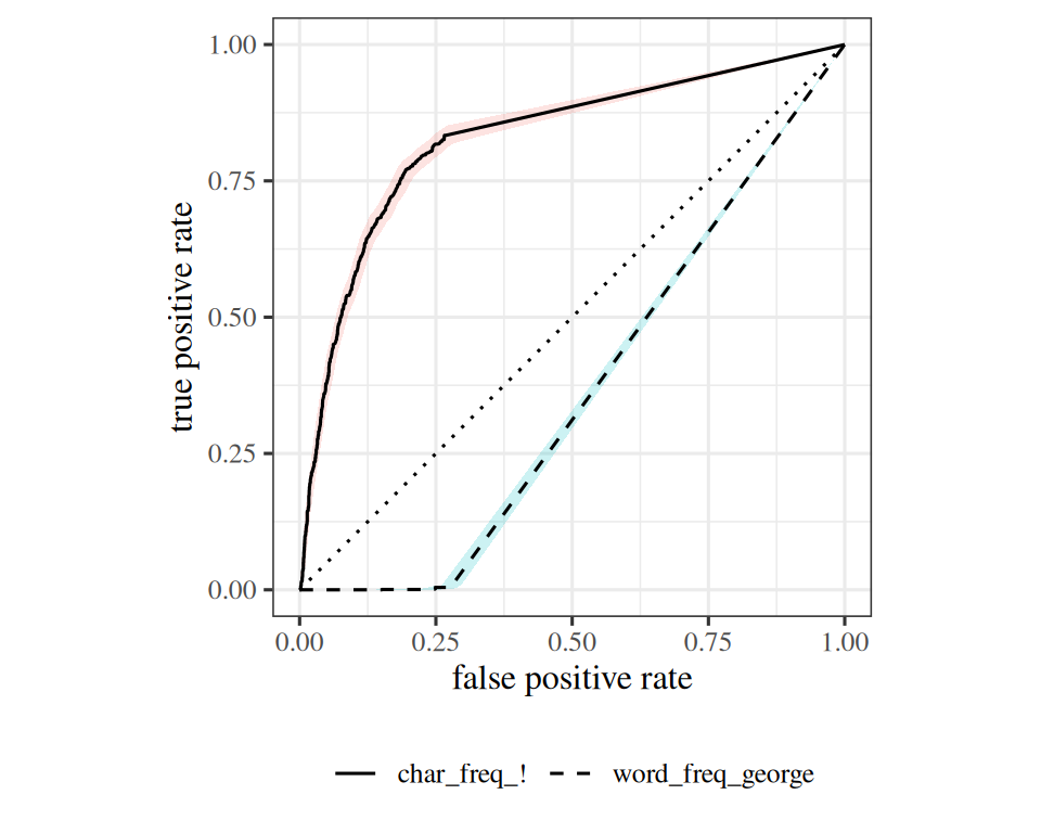
The best feature is char_freq_!, with AUC 0.83. The worst is word_freq_george, with AUC 0.36. The AUCs of the four features, with 95% bootstrap intervals, are word_freq_remove 0.70 [0.69, 0.71], word_freq_george 0.36 [0.35, 0.37], char_freq_! 0.83 [0.82, 0.84], capital_run_length_average 0.79 [0.77, 0.80]. Each interval is the middle 95% of 500 AUCs recomputed on emails drawn with replacement. Figure 2 shows the curves for the best and worst features.
ExrExercise 71 (Rank single features of real emails by ROC AUC (part 3))
Exercise 71 (Rank single features of real emails by ROC AUC (part 3)) Use the setup of Exercise 69.
Plot the ROC curves of the best and worst features on one set of axes, with the diagonal for reference.
Solution 71. See Figure 2. The curve of the best feature rises above the diagonal. The curve of the worst feature stays below it.
Show code
roc_points<-function(score, y){th<-c(Inf, sort(unique(score), decreasing =TRUE))tibble::tibble( fpr =sapply(th, function(t)mean(score[y==0]>=t)), tpr =sapply(th, function(t)mean(score[y==1]>=t)))}roc_best<-roc_points(spam_all[[best]], spam_all$Class)roc_worst<-roc_points(spam_all[[worst]], spam_all$Class)library(ggplot2)roc_df<-dplyr::bind_rows(dplyr::mutate(roc_best, feature =best),dplyr::mutate(roc_worst, feature =worst))# A bootstrap band: the true positive rate at each false positive rate on a grid,# recomputed on emails drawn with replacement. Sorting by score gives every# threshold's rates at once, so each resample is quick.fpr_grid<-seq(0, 1, length.out =101)tpr_on_grid<-function(score, y){ord<-order(score, decreasing =TRUE)# Keep one point per distinct score, the last of each tie block, so a block of# tied scores moves in one jump, as in the curve drawn from roc_points().last_of_tie<-!duplicated(score[ord], fromLast =TRUE)fpr<-c(0, (cumsum(y[ord]==0)/sum(y==0))[last_of_tie])tpr<-c(0, (cumsum(y[ord]==1)/sum(y==1))[last_of_tie])approx(fpr, tpr, xout =fpr_grid, ties ="ordered")$y}set.seed(1)band_df<-dplyr::bind_rows(lapply(c(best, worst), function(f){boot<-replicate(200, {i<-sample(nrow(spam_all), replace =TRUE)tpr_on_grid(spam_all[[f]][i], spam_all$Class[i])})tibble::tibble( fpr =fpr_grid, lower =apply(boot, 1, quantile, 0.025), upper =apply(boot, 1, quantile, 0.975), feature =f)}))ggplot(roc_df, aes(fpr, tpr, linetype =feature))+annotate("segment", x =0, y =0, xend =1, yend =1, linetype ="dotted")+geom_ribbon(aes(y =NULL, ymin =lower, ymax =upper, fill =feature), data =band_df, alpha =0.2, colour =NA, show.legend =FALSE)+geom_line()+scale_linetype_manual(values =setNames(c("solid", "dashed"), c(best, worst)))+coord_equal()+labs(x ="false positive rate", y ="true positive rate", linetype =NULL)+theme(legend.position ="bottom")
Figure 2: ROC curves on the Spambase emails for the best single feature (solid) and the worst (dashed), with the diagonal for a score that ignores the email (dotted). The worst feature’s curve lies below the diagonal. Each shaded band is a pointwise 95% bootstrap interval for the true positive rate at each false positive rate, from 200 resamples of the emails.
ExrExercise 72 (Rank single features of real emails by ROC AUC (part 4))
Exercise 72 (Rank single features of real emails by ROC AUC (part 4)) Use the setup of Exercise 69.
The feature with AUC below \(0.5\) can still be useful. Say what you would change in the rule, and what its AUC becomes.
Solution 72. Flip the rule: call an email spam when the feature is small. Negating the score swaps every pair of a spam and an email, so the new AUC is $1 - $ the old AUC, here 0.64 for word_freq_george. An AUC below \(0.5\) does not imply a feature is useless; it implies the direction of the rule is backwards. A feature with an AUC near \(0.5\) is the one that carries no information.
2.3 Differentiable
Cross-entropy (lower is better)
If \(\modmemf{x_{(i)}} \in \reals^C\) contains the posterior probabilities of the \(C\) classes and \(y_{(i)} \in \reals^C\) is a one hot vector, then \[H(y, \modmemf{x}) = -\sumiN \sumto{j}{C} y_{(i)j} \log_b \modmemf{x_{(i)}}_j\]
Exercise 73 (Reading the cross-entropy sum) A classifier outputs \(\modmemf{x_{(i)}} \in \reals^C\), a vector of posterior probabilities over the \(C\) classes, and the label \(y_{(i)} \in \reals^C\) is one-hot: it holds a 1 in the position of the true class and 0 everywhere else. The cross-entropy over a set of \(N\) examples is
Solution 73. Only the true class contributes. Write \(c_i\) for the index where \(y_{(i)}\) holds its 1. Every other \(y_{(i)j}\) is 0, so every other term of the inner sum is \(0 \cdot \log_b \modmemf{x_{(i)}}_j = 0\).
ExrExercise 74 (Reading the cross-entropy sum (part 2))
Exercise 74 (Reading the cross-entropy sum (part 2)) Use the setup of Exercise 73.
Write what Equation 1 reduces to once the one-hot structure is used.
The probabilities the classifier assigns to the wrong classes never appear. They matter only because the vector sums to 1, so probability spent on a wrong class is probability taken from the right one.
ExrExercise 75 (Reading the cross-entropy sum (part 3))
Exercise 75 (Reading the cross-entropy sum (part 3)) Use the setup of Exercise 73.
What is the smallest value \(H\) can take, and what must the classifier do to reach it?
Solution 75. The smallest value is 0. A probability is at most 1, so \(\log_b \modmemf{x_{(i)}}_{c_i} \le 0\) and each term of the sum above is at least 0. Equality needs \(\modmemf{x_{(i)}}_{c_i} = 1\) for every \(i\): the classifier must put all of its probability on the true class, every time.
ExrExercise 76 (Reading the cross-entropy sum (part 4))
Exercise 76 (Reading the cross-entropy sum (part 4)) Use the setup of Exercise 73.
Solution 76. There is no largest value. As \(\modmemf{x_{(i)}}_{c_i} \to 0\), \(-\log_b \modmemf{x_{(i)}}_{c_i} \to \infty\). One confident mistake is enough: a classifier that assigns the true class a probability of \(10^{-12}\) on a single example contributes 12 hartleys from that example alone. This asymmetry is the metric working as intended. Accuracy charges 1 for a mistake whether the classifier was hesitant or certain; cross-entropy charges for the certainty.
ExrExercise 77 (Reading the cross-entropy sum (part 5))
Exercise 77 (Reading the cross-entropy sum (part 5)) Use the setup of Exercise 73.
The base \(b\) names the units: 2 gives bits, \(e\) gives nats, 10 gives hartleys. Show that changing \(b\) multiplies \(H\) by a positive constant, and say what that implies for comparing two classifiers.
Solution 77. The base is a scale factor. By the change-of-base identity, \(\log_b z = \ln z / \ln b\), so
\[
H_b = \frac{H_e}{\ln b},
\]
and \(\ln b > 0\) for any \(b > 1\). So the three unit choices give three numbers that are positive multiples of each other: 1.386 nats is 2 bits is 0.602 hartleys.
Multiplying every score by the same positive constant leaves their order alone, so a classifier that beats another in bits beats it in nats too, and the base cannot change which model you pick. It changes only the units in which the number is expressed.
Theorem 1 (Cross-entropy with one-hot labels) Let each label \(y_{(i)}\) be one-hot, with its 1 at position \(c_i\). Then the cross-entropy of Equation 1 reduces to the negative log probability that the classifier assigns to the true class of each example:
Example 1 A classifier with \(C = 3\) classes outputs \(\modmemf{x} = (\tfrac12, \tfrac14, \tfrac14)\) for one example. In bits (\(b = 2\)), Equation 2 gives \(-\log_2 \tfrac12 = 1\) if the true class is the first, and \(-\log_2 \tfrac14 = 2\) if it is the second or the third. The probability on the other two classes never enters.
LemTheorem 2 (Cross-entropy with one-hot labels is nonnegative)
Theorem 2 (Cross-entropy with one-hot labels is nonnegative) With one-hot labels, the cross-entropy of Equation 1 satisfies \(H(y, h(x)) \ge 0\). It equals \(0\) exactly when the classifier puts probability \(1\) on the true class of every example.
Example 2 (Cross-entropy of two classifiers) On two examples, a classifier assigns the true class the probabilities \(0.8\) and \(0.5\). A second classifier assigns it \(1\) and \(1\).
Show code
cn_true_prob<-list(first =c(0.8, 0.5), second =c(1, 1))vapply(cn_true_prob, \(p)-sum(log2(p)), numeric(1))
   first   second
1.321928 0.000000
By Theorem 2 both values are at least \(0\). The first classifier scores 1.322 bits. The second scores exactly \(0\), because it puts all its probability on the true class every time.
LemTheorem 3 (Changing the base of cross-entropy rescales it)
Theorem 3 (Changing the base of cross-entropy rescales it) Let \(H_b\) be the cross-entropy of Equation 1 in base \(b > 1\). Then
\[
H_b = \frac{H_e}{\ln b}.
\]
Two classifiers are therefore ordered the same way in every base.
The second row is \(H_e / \ln b\) for \(b = 2, e, 10\), and by Theorem 3 it matches the first row. Every classifier’s score is multiplied by the same \(1/\ln b\), so the ordering of classifiers does not change with the base.
NoteOther names for cross-entropy, and two conventions to state
Software and statistics each renamed this quantity. Log loss and logistic loss are the same number, and so is the negative log-likelihood of the labels under the model, since \(-\log \modmemf{x_{(i)}}_j\) at the true class \(j\) is exactly the log-likelihood of that label with its sign reversed. Generalized linear models add deviance, which for one-hot labels is twice the summed negative log-likelihood.
Settle two conventions before comparing one of these numbers with another source’s. The notation choices page explains both.
Which base. The definition of \(H\) leaves the base \(b\) free. Theorem 3 shows the base cannot change which of two classifiers you would pick, but it does change the number itself, so state the base whenever you quote one.
Summed or averaged. The chapter’s \(H(y, \modmemf{x})\) sums over all \(N\) examples. Most software reports the mean, \(\bar H = H/N\), under the same name. The chapter is explicit about this where it matters: perplexity is defined from \(\bar H\), not from \(H\).
where \(\bar H\) is the per-example cross-entropy of Equation 1 rather than the sum.
Take a classifier that spreads its probability evenly over all \(C\) classes on every example. Compute \(\bar H\) and then \(ppl\). Do it in bits and again in hartleys.
Solution 78. The even classifier has perplexity \(C\). Every predicted probability is \(1/C\), so by Equation 2 each example contributes \(-\log_b (1/C) = \log_b C\), and the average is \(\bar H = \log_b C\). Then
The base cancels: it enters once in the units of \(\bar H\) and once as the base of the exponent, and the two uses undo each other. So perplexity is quoted as a bare number where cross-entropy has to be quoted with its units.
with equality exactly when \(\bar H = 0\) — the classifier that is always certain and always right. Perplexity is bounded below by 1 rather than 0 because it counts options, and there is always at least one.
Exercise 81 (What perplexity counts (part 4)) Use the setup of Exercise 78.
Exercise 78 is where the usual explanation comes from: a perplexity of \(k\) implies the classifier is as uncertain as someone choosing among \(k\) equally likely options. A language model reports a per-word perplexity of 20 over a vocabulary of 50,000 words. Say what that does and does not tell you.
Solution 81. It reports difficulty, not vocabulary. A perplexity of 20 says the model is, on average, as uncertain about the next word as someone choosing uniformly among 20 candidates. The gap between 20 and 50,000 is the model’s whole contribution: context has narrowed 50,000 options down to about 20.
Three things it does not tell you. It is an average, so a model that is nearly certain on function words and uncertain about content words can report the same 20 as one that is moderately uncertain about every word. It says nothing about whether the 20 candidates include the right word at all. And it is comparable across two models only when they share a vocabulary and a tokenizer: a model that splits words into smaller pieces is predicting easier things more often, so its per-token perplexity is lower without the model being better.
The sum of squared errors (SSE) adds up the squared distances between predictions and labels. Dividing by \(N\) gives the sample mean squared error (sMSE), and its square root is the sample root mean squared error (sRMSE):
\(SSE\) is also the sum of squared residuals or the residual sum of squares (\(RSS\)). \(\sMSEt\) is also the quadratic loss, and \(\sRMSEt\) is the root mean square of the residuals.
\(L_2\) loss names this family too, and is the one to define before using. Some sources mean \(\sMSEt\) by it and some mean \(SSE\). Those two losses rank models identically on a fixed dataset, since they differ by the constant factor \(N\), and \(\sRMSEt\) ranks with them for the same reason: the square root is applied once, at the end, and is increasing.
A third reading is a different objective, not a different scale. Some sources take the root inside the sum, scoring a model by \(\sum_i\norm{ \eoutvar_{(i)} - \outvar_{(i)}}_2\). Moving the root inside changes which model wins, because each un-squared distance then enters the sum on its own rather than being squared first.
Solution 82. Only \(\sRMSEt\) is in dollars. A residual is a difference of rents, so it is in dollars; squaring gives dollars squared. \(SSE\) and \(\sMSEt\) are therefore both in dollars squared, and the square root returns \(\sRMSEt\) to dollars.
That is the whole case for \(\sRMSEt\): a report of $180 can be compared with a rent of $1,400, where a report of 32,400 dollars-squared can be compared with nothing the reader knows.
ExrExercise 83 (Three names for one quantity (part 2))
Exercise 83 (Three names for one quantity (part 2)) Use the setup of Exercise 82.
Two analysts fit the same model to the same data. One evaluates on all 1,000 apartments, the other on a random half of them. Which of the three quantities do you expect to differ, and which to agree?
Solution 83. \(SSE\) differs; \(\sMSEt\) and \(\sRMSEt\) roughly agree.\(SSE\) adds one non-negative term per example, so halving the evaluation set roughly halves it. It measures the dataset as much as the model. \(\sMSEt\) divides that total by \(N\), which cancels the dependence on how many apartments were scored, and \(\sRMSEt\) inherits the cancellation.
So \(SSE\) is the quantity to minimize during fitting, where \(N\) is fixed and the constant factor is irrelevant, and \(\sMSEt\) or \(\sRMSEt\) is the quantity to report, where the reader’s evaluation set is not yours.
ExrExercise 84 (Three names for one quantity (part 3))
Exercise 84 (Three names for one quantity (part 3)) Use the setup of Exercise 82.
A residual of 0.5 and a residual of 2 both contribute to \(SSE\). Compare each contribution to the size of the residual itself, and state the general rule.
Solution 84. Squaring shrinks residuals below 1 and stretches those above.\(0.5^2 = 0.25\), which is half of 0.5. \(2^2 = 4\), which is twice 2. In general \(e^2 <\abs{ e}\) when \(\abs{ e} < 1\) and \(e^2 >\abs{ e}\) when \(\abs{ e} > 1\), with the two agreeing at \(\abs{ e} = 1\).
Note what the crossover depends on: the unit. The same rents measured in cents put every residual far above 1, and the same rents measured in thousands of dollars put most of them below it. The rule is about the number, not about the error being small.
ExrExercise 85 (Three names for one quantity (part 4))
Exercise 85 (Three names for one quantity (part 4)) Use the setup of Exercise 82.
Exercise 84 is often summarized as “squaring penalizes large errors.” Name a situation where that is the behavior you want, and one where it is not.
Solution 85. It depends on what a large error costs. Squaring is right when the cost of being wrong grows faster than the error does. A delivery estimate that is 10 minutes late is an annoyance; one that is 100 minutes late may cause the customer to leave, and that is worse than ten annoyances.
It is wrong when the large residuals are not real. One mistyped rent of $14,000 instead of $1,400 contributes a residual near 12,600, whose square exceeds the combined squares of four thousand ordinary residuals of $180 — so the fit moves to accommodate a typo. Exercise 86 covers what to do instead.
ReadingRead
GeeksforGeeks explains regression metrics[21], including MSE, RMSE and MAE (its names for the sMSE, sRMSE and sMAE).
3.2 sMAE
The sample mean absolute error (sMAE) replaces the squares with absolute values:
Take the simplest possible regression, \(C = 1\) and no inputs at all, so the model is a single constant \(c\) and \(\norm{ \modmem - y}_1 =\abs{ c - y}\). The five observations are
\[
2, \quad 3, \quad 4, \quad 5, \quad 100 .
\]
Find the \(c\) that minimizes \(\sMSEt\), and the \(c\) that minimizes \(\sMAEt\). Name each in one word.
Solution 86. The mean and the median. Squared error is minimized by the mean, \((2+3+4+5+100)/5 = 22.8\). Absolute error is minimized by the median, 4.
The gap is the whole lesson. Four of the five observations lie between 2 and 5, and the squared-error fit lands at 22.8 — above every one of them. No observation is anywhere near the value that best summarizes them under \(\sMSEt\).
ExrExercise 87 (What changes when you fit with absolute error (part 2))
Exercise 87 (What changes when you fit with absolute error (part 2)) Use the setup of Exercise 86.
Differentiate \(\sum_{i}\abs{ c - \outvar_{(i)}}\) with respect to \(c\) at a point where \(c\) equals none of the observations, and say what setting the derivative to zero requires.
Solution 87. Zero requires a tie in the counts. Away from the observations, \(\abs{ c - y_{(i)}}\) is differentiable with derivative \(+1\) when \(c > y_{(i)}\) and \(-1\) when \(c < y_{(i)}\). Summing,
\[
\frac{d}{dc} \sumiN \abs{ c - y_{(i)} }
= \#\{ i : y_{(i)} < c \} - \#\{ i : y_{(i)} > c \} .
\]
Setting this to zero would require as many observations below \(c\) as above it, and with \(N = 5\) the two counts sum to an odd number, so their difference is never zero. No off-observation point is stationary. The derivative is \(-1\) just left of \(4\) and \(+1\) just right of it, so the sum falls until \(c\) reaches \(4\) and rises after: the minimum sits at that corner, not at a stationary point.
Notice what the derivative does not contain: the values \(y_{(i)}\) themselves, only their side of \(c\). Moving the 100 to 10,000 leaves every count unchanged, so the \(\sMAEt\) fit does not move at all. The \(\sMSEt\) derivative is \(2\sum (c - y_{(i)})\), which carries every value, so the same edit moves the mean from 22.8 to 2,002.8.
ExrExercise 88 (What changes when you fit with absolute error (part 3))
Exercise 88 (What changes when you fit with absolute error (part 3)) Use the setup of Exercise 86.
Which of the two answers in Exercise 86 would you rather report as the typical rent, and why?
Solution 88. The median, for a typical rent. A reader who hears “typical” expects a value that describes most of the apartments. 4 does; 22.8 describes none of them. The mean is answering a different question — what you would pay per apartment if you rented all five — which is the right question for a budget and the wrong one for a description.
ExrExercise 89 (What changes when you fit with absolute error (part 4))
Exercise 89 (What changes when you fit with absolute error (part 4)) Use the setup of Exercise 86.
Solution 89. Squared error is smoother and has a closed-form solution.\(\sMSEt\) is differentiable everywhere, and for linear models the minimizer is a formula. \(\sMAEt\) has a corner at every observation, where the derivative jumps from \(-1\) to \(+1\) without passing through intermediate values, so gradient methods need care and there is generally no closed-form solution.
The choice is a statement about the data. Squared error assumes the extreme observations are real and worth fitting; absolute error assumes they are noise and should not move the answer. With 100 as a genuine penthouse, the mean is informative. With 100 as a typo for 10.0, it is a fit ruined by one keystroke.
NoteOther names for sMAE, and one abbreviation that is not it
\(\sMAEt\) is also the \(L_1\) loss and the mean absolute deviation.
That second name suggests the abbreviation MAD, which is ambiguous: forecasting uses it for the mean absolute deviation, and much statistical writing uses it for the median absolute deviation, \(\operatorname{median}_i\abs{ y_{(i)} - \operatorname{median}(y)}\), which measures how spread out a single sample is. That second quantity takes no model and no predictions, where \(\sMAEt\) measures how far a model’s predictions fall from the truth. The two readings of MAD share an abbreviation, two of their three words, and nothing else. Expand MAD the first time you write it.
3.3\(R^2\)
The coefficient of determination (sometimes written \(r^2\)) measures how much of the variance in the output we can predict from the input variable(s).
NoteTwo near-synonyms for \(R^2\), and two names that mean different things in different sources
Squared correlation. Writing \(R^2\) as \(r^2\) suggests it is the Pearson correlation squared, and for a least-squares fit with an intercept it is. Outside that case the two are different quantities, and Exercise 91 examines the range of \(R^2\). Anything that reports \(r^2\) for a model you did not fit by least squares with an intercept is reporting a different quantity under a familiar name.
Explained variance. Some libraries report a score by that name which replaces \(SSE/N\) with the variance of the residuals. The two agree whenever the residuals average to zero, which a least-squares fit with an intercept guarantees, so the distinction stays invisible until a model is biased. Take \(y = (2, 4, 6, 8, 10)\) and a model that predicts \(y + 1\) for every point. Every residual is \(-1\), so the residuals have zero variance and a score computed that way is \(1\), a perfect fit, while \(R^2\) is \(1 - 5/40 = 0.875\). One score is measuring the shape of the predictions and the other is measuring the predictions.
\(SSR\) and \(ESS\).\(SS_{tot}\) splits into the part a least-squares fit with an intercept explains and the part it leaves over, and the abbreviations for those two pieces are not standardized. \(SSR\) is read as the regression sum of squares by some sources and as the residual sum of squares by others, which are the two different pieces; \(ESS\) is read as explained by some and as error by others, likewise. Do not infer either from the letters. Read which piece the source subtracts from \(SS_{tot}\), or which one it puts in the numerator of \(1 - (\cdot)/SS_{tot}\).
ExrExercise 90 (When the coefficient of determination goes negative)
Exercise 90 (When the coefficient of determination goes negative) The coefficient of determination compares your model’s squared error against the squared error of one particular comparison model:
Solution 90. The comparison model is the constant model that always predicts \(\bar y\). Substituting \(\eoutvar_{(i)} = \bar y\) into \(SSE\) gives exactly \(SS_{tot}\). So \(R^2\) asks one question: by what fraction does your model reduce the squared error of a model that ignores the inputs entirely?
\(R^2 = 0\) means it reduces it by none. The model is worth exactly what the average of the labels is worth, whatever its inputs, parameters or training cost.
ExrExercise 91 (When the coefficient of determination goes negative (part 2))
Exercise 91 (When the coefficient of determination goes negative (part 2)) Use the setup of Exercise 90.
\(R^2\) is often introduced as a proportion of variance, which would put it between 0 and 1. Show that Equation 6 can go negative, using \(\outvar = (1, 2, 3, 4)\) and a model that predicts 10 everywhere.
Nothing is out of range, because \(R^2\) is not a proportion of anything. It is 1 minus a ratio of two error sums, and that ratio is unbounded above. The proportion-of-variance reading is a special case, true only when the model was fit by least squares with an intercept and is being scored on the data it was fit to. If any of those three conditions fails, the lower bound of 0 no longer holds.
ExrExercise 92 (When the coefficient of determination goes negative (part 3))
Exercise 92 (When the coefficient of determination goes negative (part 3)) Use the setup of Exercise 90.
Solution 93. Write \(\bar \outvar_{\text{train}}\) for the trainingmean and \(\bar \outvar\) for the test mean. The modelpredicts\(\bar \outvar_{\text{train}}\) for every test point, so
\[
\begin{aligned}
SSE
&= \sumiN \paren{ y_{(i)} - \bar y_{\text{train}} }^2 \\
&= \sumiN \paren{ y_{(i)} - \bar y }^2 + N \paren{ \bar y - \bar y_{\text{train}} }^2 \\
&= SS_{tot} + N \paren{ \bar y - \bar y_{\text{train}} }^2 .
\end{aligned}
\]
The middle term vanishes because the differences \(\outvar_{(i)} - \bar \outvar\) sum to zero. Then
This is zero only when the means agree. Otherwise it is negative: the model is worse than the model that predicts the sample mean of the test set’s labels for every point.
ExrExercise 94 (When the coefficient of determination goes negative (part 5))
Exercise 94 (When the coefficient of determination goes negative (part 5)) Use the setup of Exercise 90.
A test set has \(N = 50\) points and \(SS_{tot} = 200\). A model scores \(R^2 = 0.75\) on it. Find \(SSE\) and \(\sMSEt\) on the test set.
On a fixed test set, a higher \(R^2\) implies a smaller \(\sMSEt\). Across different problems that link breaks. \(R^2\) is scaled by how much the labels vary, so predicting rents in a city where they range from $800 to $5,000 is an easier way to earn a high \(R^2\) than predicting them in a block where they range from $1,400 to $1,500. The second model can have the far smaller \(\sMSEt\) while reporting the far worse \(R^2\). Report both.
ExrExercise 95 (Plot predictions against the true outputs)
Exercise 95 (Plot predictions against the true outputs) The Auto data give the fuel economy mpg and the horsepower of 392 cars. Use the copy data/auto.csv on this site. Any computer with R or Python can run the code in the solution.
Solution 98. If every prediction were perfect, the points would lie on the dashed line, where the prediction equals the true value. The distance from a point to that line, measured vertically, is the point’s residual.
ExrExercise 99 (Plot predictions against the true outputs (part 5))
Exercise 99 (Plot predictions against the true outputs (part 5)) Use the setup of Exercise 95.
The plot of Exercise 97 should show a pattern. Say what the pattern is, and what it tells you about the line.
Solution 99. In the plot of Exercise 97, the points for the line bend away from the dashed line instead of following it. The line predicts too low for the cars with the highest mpg and too high for many cars in the middle of the range. A residual pattern like this shows that the model’s mistakes are systematic, not noise: fuel economy falls with horsepower along a curve, and a straight line cannot follow it. A single number such as the sample \(R^2\) of 0.606 does not show this, and the plot does.
ExrExercise 100 (Plot predictions against the true outputs (part 6))
Exercise 100 (Plot predictions against the true outputs (part 6)) Use the setup of Exercise 95.
Predicted against true miles per gallon for the Auto cars, from a line (left) and a quadratic (right) in horsepower. The dashed line is where the prediction equals the true value.
fit_quad<-lm(mpg~poly(horsepower, 2), data =auto_r)cat("quadratic R^2 =", round(r2_r(auto_r$mpg, fitted(fit_quad)), 3), "\n")
Predicted against true miles per gallon for the Auto cars, from a line (left) and a quadratic (right) in horsepower. The dashed line is where the prediction equals the true value.
ExrExercise 101 (Plot predictions against the true outputs (part 7))
Exercise 101 (Plot predictions against the true outputs (part 7)) Use the setup of Exercise 95.
Solution 101. With the quadratic, the points scatter more evenly around the dashed line. A predicted-versus-true plot plays the role for regression that the confusion matrix plays for classification: it shows what kind of mistakes the model makes, not only how many.
ExrExercise 102 (Plot predictions against the true outputs (part 8))
Exercise 102 (Plot predictions against the true outputs (part 8)) Use the setup of Exercise 95.
Solution 102. With the quadratic, the sample \(R^2\) rises to 0.688.
4 Token Sequences
4.1 Token Error Rate
Our model outputs a hypothesis sequence, and we compare it to a reference sequence.
Rather than comparing tokens at matching indices, we compute an edit distance. The edit distance lets us substitute, delete or insert tokens, but not reorder them.
Commonly used to evaluate speech recognition systems.
Perform a minimum edit distance alignment of the reference sequence (length \(N_{ref}\)) to the hypothesis sequence (length \(N_{hyp}\)).
Count substitutions (\(S\)), insertions (\(I\)) and deletions (\(D\)).
Compute the token error rate (TER) as follows: \[TER = \frac{S + I + D}{N_{ref}}\]
NoteOther names for TER, and a second meaning of the acronym
The rate takes its name from whatever the tokens are. Words give word error rate (WER), characters give character error rate (CER), and phones give phone error rate (PER). The distance the alignment step minimizes is an edit distance or a Levenshtein distance, the two naming one quantity when substituting, inserting and deleting each cost one.
A published number needs two checks before you compare yours to it: what that source counts as an edit, and what it expands TER to. Machine translation uses the same three letters for a translation edit rate, which allows a block of tokens to be moved as a single edit. The edit distance in this chapter does not: reordered output is charged as deletions and insertions instead. A rate computed under the two rules is not the same measurement. The rule that allows moves can never score higher, since every alignment without a move is still available to it, and it scores strictly lower whenever a move beats the deletions and insertions it replaces.
ExrExercise 103 (Scoring a sequence against a reference)
Exercise 103 (Scoring a sequence against a reference) A speech recognizer outputs a hypothesis sequence, which you want to score against a reference sequence. Token error rate aligns the two by minimum edit distance, counting substitutions \(S\), insertions \(I\) and deletions \(D\), and reports
\[
TER = \frac{S + I + D}{N_{ref}} .
\tag{7}\]
The edit distance allows tokens to be substituted, deleted or inserted, but not reordered.
Take the reference the cat sat on the mat and the hypothesis the cat sit on mat. Find the alignment and give \(S\), \(I\) and \(D\).
Solution 103. The alignment finds one substitution and one deletion.
Table 3: The minimum-edit alignment
Reference
the
cat
sat
on
the
mat
Hypothesis
the
cat
sit
on
—
mat
In Table 3 the token sat became sit, a substitution, and the second the is missing, a deletion. So \(S = 1\), \(I = 0\) and \(D = 1\). No alignment does it in fewer edits: the sequences differ in length, which forces at least one deletion, and sat and sit differ, which forces at least one more.
ExrExercise 104 (Scoring a sequence against a reference (part 2))
Exercise 104 (Scoring a sequence against a reference (part 2)) Use the setup of Exercise 103.
Compute \(TER\) by Equation 7 for the alignment you found there.
Solution 105. The smallest value is 0. Each of \(S\), \(I\) and \(D\) is a count, so the numerator is at least 0, and it is 0 exactly when the two sequences are identical.
ExrExercise 106 (Scoring a sequence against a reference (part 4))
Exercise 106 (Scoring a sequence against a reference (part 4)) Use the setup of Exercise 103.
What is the largest? If there is no largest, give a hypothesis that exceeds 1.
Solution 106. There is no largest value. The numerator counts edits, which insertions make unbounded, while the denominator is fixed by the reference alone. Take a one-token reference and a hypothesis of 100 wrong tokens: one substitution and 99 insertions give
\[
\begin{aligned}
TER &= 100/1 \\
&= 100.
\end{aligned}
\]
A rate above 1 is not a paradox here, because \(TER\) is not a proportion of anything — the same structure as \(R^2\) in Exercise 90, and the same warning. A name ending in rate invites the reader to assume a ceiling that the definition does not provide.
ExrExercise 107 (Scoring a sequence against a reference (part 5))
Exercise 107 (Scoring a sequence against a reference (part 5)) Use the setup of Exercise 103.
Exercise 106 exposes an asymmetry in Equation 7. Name it, and say what it costs a recognizer that is unsure whether it heard a word.
Solution 107. Inserting is charged, and staying silent is charged the same.\(N_{ref}\) does not grow when the hypothesis does, so a recognizer is charged one unit for a word it guesses wrongly and one unit for a word it omits. Write \(p\) for the chance a word really is there, and \(q\) for the chance a guess names it correctly when it is. Guessing costs \(1 - pq\), since it escapes the charge only when the word is present and the guess is right. Silence costs \(p\), since an omission is charged only when there was something to omit. So guessing is better when \(pq > 1 - p\), which needs \(p\) well above a half: a recognizer unsure whether it heard anything at all gains nothing by guessing, whatever \(q\) is. The asymmetry rewards a different case, the one where a word is certainly there and only its identity is in doubt. There \(p\) is near 1, silence costs almost a full unit, and any guess with \(q > 0\) beats it. A system tuned on \(TER\) will fill those stretches with its best guess rather than leave a gap.
Whether that is the behavior you want depends on the reader of the transcript. For a search index it is: a wrong word is skipped, a missing word cannot be found. For a medical dictation it is not, where a confident wrong drug name is worse than a blank a clinician can see and fill. The metric cannot make that judgment, so it has to be made before the metric is chosen.
K. H. Brodersen, C. S. Ong, K. E. Stephan, and J. M. Buhmann, “The balanced accuracy and its posterior distribution,” in 20th international conference on pattern recognition (ICPR), 2010, pp. 3121–3124. doi: 10.1109/ICPR.2010.764.
T. Hastie, R. Tibshirani, and J. Friedman, The elements of statistical learning: Data mining, inference, and prediction, 2nd ed. Springer, 2009. Available: https://hastie.su.domains/ElemStatLearn/