Regularization

Published

Last modified: 2026-10-28

Show code
# The Python chunks on this page import numpy, pandas and matplotlib;
# reticulate provisions them.
# The Julia chunks run through JuliaCall.
library(reticulate)
py_require(c("numpy", "pandas", "scipy", "matplotlib"))

Consolidated from Brian Hutchinson’s Fall 2025 topic notes and Kameron Decker Harris’ 2022 weekly notes, and drawing on Logan Sizemore’s Spring 2025 lecture on regularization for the data-augmentation section.

1 Why regularize

Linear regression can still give unstable estimates. Correlated features, for example, can take large but offsetting weights. We regularize to favor simple solutions: we penalize large coefficients, and so penalize more complicated models.

ReadingRead

GeeksforGeeks explains regularization [1].

ExrExercise 1 (Brainstorm remedies for overfitting)

Exercise 1 (Brainstorm remedies for overfitting) A model fits its training data very well and a held-out set poorly. List the ways you can think of to make it generalize better. For each, say what it changes: the data, the model, or the training procedure.

Solution 1.

  • The data. Collect more training examples, so that noise is harder to fit. Augment the existing examples with label-preserving transformations (see Regularizing without a penalty, below).

  • The model. Use fewer features or a lower polynomial degree, so the model has less freedom to chase noise. Penalize large coefficients, as ridge regression (ridge for short) and the lasso (least absolute shrinkage and selection operator) do. Both are the subject of this chapter.

  • The training procedure. Stop training when a held-out score stops improving (early stopping), or train an ensemble or use dropout so that no single fitted copy has to be right.

  • Choosing among these. Whichever remedy has a tuning parameter, such as the penalty \(\regpar\), the degree, or the stopping time, set it by cross-validation rather than by the training error. The training error always favors using less of the remedy.

All of them trade a little bias for less variance.

2 Features and polynomial regression

Before regularizing, note what makes the problem badly conditioned in the first place. Fitting a polynomial is still linear regression, but in expanded features:

Model (Polynomial Regression) \[F(x) = \coef{0} + \coef{1} x + \coef{2} x^2 + \coef{3} x^3 + \dots + \coef{p} x^p\] \[\min_{\vcoef} \sumin \paren{F(x_i) - y_i}^2\] \[\min_{\vcoef} \sumin \paren{\coef{0} + \coef{1} x_i + \dots + \coef{p} x_i^p - y_i}^2\] \[\min_{\vcoef} \norm{ \design \vcoef - \vy }^2\]

Those three displays are one optimization problem written three ways: the second names the model, the third expands it, and the fourth stacks the expanded features into the matrix \(\design\) of Equation 1.

Feature Matrix \(\design\) \[\design = \begin{bmatrix} 1 & x_1 & x_1^2 & \cdots & x_1^p \\ 1 & x_2 & x_2^2 & \cdots & x_2^p \\ \vdots & \vdots & \vdots & & \vdots \\ 1 & x_n & x_n^2 & \cdots & x_n^p \end{bmatrix}_{\,n\times(p+1)} \tag{1}\]

  • Need \(n > p\) to fit with linear regression.

  • If \(p\) is large relative to \(n\), then \(\design^\top\design\) is close to singular.

Here the degree \(p\) is the number of non-constant columns of \(\design\). The condition \(n > p\) is the one stated in Linear Regression.

The same expansion works in more than one input dimension. For \(\vx = (x_1, x_2)\):

\[F(\vx) = \coef{0} + \coef{1} x_1 + \coef{2} x_2 + \coef{3} x_1^2 + \coef{4} x_2^2 + \coef{5} x_1 x_2\]

VideosWatch

Hastie and Tibshirani explain polynomial features [2], video 7.1.

ReadingRead

GeeksforGeeks explains polynomial regression [3].

3 Underdetermined problems

Keep the padding convention of Linear Regression: \(X\) carries \(\ninputvars\) feature columns plus an intercept column, so it is \(n \times (\ninputvars+1)\). Its rank is at most \(n\), so when \(n \le \ninputvars\) the columns are linearly dependent, \(X^\top X\) is singular, and the cost function is flat along some directions — there are many solutions rather than one. (The \(n\) data vectors themselves are generically independent, but the feature columns are linearly dependent.)

The fix is to add a regularization term:

\[\boxed{\displaystyle \sumin \paren{y_i - x_i^T\regcoef}^2 + \regpar \sumto{j}{\ninputvars} \coef{j}^2}\]

The loss term has elliptical contours; the penalty term has circular contours centered at \(\vzero\).

VideosWatch

Abu-Mostafa teaches regularization [4], Lecture 12.

4 Ridge regression

Ridge regression — Hoerl and Kennard [5] — adds a penalty on the size (\(\ell_2\) norm) of \(\vcoef\):

\[\argmin_{\vcoef} (y - X\vcoef)^T (y - X\vcoef) + \regpar \underbrace{\norm{\vcoef}^2}_{\vcoef^T \vcoef}\]

or equivalently

\[\boxed{\displaystyle \vcoef_{\text{ridge}}(\regpar) = \argmin_{\vcoef} \norm{ X\vcoef - \vy }^2 + \regpar \norm{ \vcoef }^2}\]

where the first term is the loss function and the second is the regularization term (penalty). The assumption behind ridge regression is that the response will vary more in directions of high variance in the input. We write the objective function being minimized, or objective for short, as

\[J_{\text{ridge}}(\vcoef) = \norm{ X\vcoef - \vy }^2 + \regpar \norm{ \vcoef }^2\]

matching the \(J\) used for the unpenalized cost in Linear Regression.

ExrExercise 2 (Follow ridge through the bias-variance tradeoff)

Exercise 2 (Follow ridge through the bias-variance tradeoff) Suppose you fit ridge regression with an unpenalized intercept, and you let the penalty weight \(\regpar\) run from \(0\) to very large. For each end of that range, say what the fitted model becomes, and whether the bias and the variance of its predictions are high or low.

Solution 2. \(\regpar \to 0\). The penalty vanishes and ridge becomes ordinary least squares. If the model form is right, the bias is low, but the coefficients can swing a lot from one training set to another, especially with many or correlated features, so the variance is high.

\(\regpar \to \infty\). Any nonzero coefficient adds more penalty than it removes in squared error, so every penalized coefficient shrinks toward \(0\). Only the intercept survives, and the model predicts the same constant, the mean of the training responses, for every input. That prediction barely changes between training sets, so the variance is low, but it ignores the features, so the bias is high unless the true relationship is flat.

ExrExercise 3 (Follow ridge through the bias-variance tradeoff (part 2))

Exercise 3 (Follow ridge through the bias-variance tradeoff (part 2)) Use the setup of Exercise 2.

What does an intermediate \(\regpar\) give?

Solution 3. Intermediate \(\regpar\). Shrinking trades some bias for a reduction in variance. When the variance saved is larger than the squared bias added, the expected squared error on new data falls, so a moderate \(\regpar\) often predicts better than either end. Choosing it is a model-selection problem, usually solved by cross-validation.

4.1 Closed-form solution

Setting the gradient to zero:

\[ \begin{aligned} \grad_{\vcoef} J_{\text{ridge}} &= 2X^\top X\vcoef - 2X^\top\vy + 2\regpar\vcoef \\ &= \vzero \end{aligned} \]

Divide through by \(2\):

\[X^\top X\vcoef - X^\top\vy + \regpar\vcoef = \vzero\]

Move the term in \(\vy\) to the right-hand side, then collect the two terms in \(\vcoef\) by factoring out the vector:

\[X^\top X\vcoef + \regpar\vcoef = X^\top\vy\] \[\paren{X^\top X + \regpar I}\vcoef = X^\top\vy\]

The \(I\) appears because \(\regpar\vcoef = \regpar I \vcoef\): to add a scalar multiple of \(\vcoef\) to a matrix times \(\vcoef\), write the scalar as a matrix first. Solving gives

\[\boxed{\displaystyle \vcoef_{\text{ridge}} = \paren{X^\top X + \regpar I}^{-1} X^\top \vy} \tag{2}\]

Never take a matrix inverse; in practice, use a solver instead.

4.2 Choosing \(\regpar\)

  • As \(\regpar \uparrow\), \(\vcoef \downarrow\) — underfit

  • As \(\regpar \downarrow\), \(\vcoef \uparrow\) — overfit

Picking \(\regpar\) is a model selection problem; see Model Selection. Exercise 8 chooses it by cross-validation, and applies the one-standard-error rule.

4.3 Practical considerations

1. Standardize features. If we use ridge, we want our features scaled to be comparable:

\[X = \begin{bmatrix} 500{,}000 & 65 \\ 30{,}000 & 26 \\ 20{,}000 & 23 \\ \vdots & \vdots \end{bmatrix} \begin{matrix} \\ \text{Income} \quad \text{Age} \end{matrix}\]

\(\displaystyle x_{ij} \rightarrow \frac{x_{ij} - \mean_j}{\sdpar_j}\) \(\mean_j = \dfrac{1}{n}\sumin x_{ij}\), \(\varpar_j = \dfrac{1}{n-1}\sumin (x_{ij} - \mean_j)^2\)

2. Don’t penalize the intercept term. Replace the \(I\) in the closed form with the identity whose first diagonal entry we set to zero, which we write \(I_0\) here.

\[\paren{X^\top X + \regpar I_0}\vcoef = X^\top\vy, \qquad \regpar I_0 = \begin{bmatrix} 0 & & \\ & \regpar & \\ & & \ddots \\ & & & \regpar \end{bmatrix}\]

Shrinking the intercept would pull every prediction toward zero. That would reflect the units the outcome happens to be measured in, not the model.

4.4 In code

Both practical considerations at once: standardize, build \(I_0\), and solve \(\paren{X^\top X + \regpar I_0}\vcoef = X^\top\vy\) for a range of \(\regpar\). Income and age are on very different scales here, so this example needs the standardizing step.

Watch what the printed coefficients do as \(\regpar\) increases. The two slopes shrink toward zero, as the penalty intends. The intercept does not move at all, a stronger result than “it is unpenalized”. Once the feature columns are centered, they are orthogonal to the column of ones, so the intercept decouples from the rest of the system and equals \(\bar{y}\) for every \(\regpar\).

import numpy as np

rng = np.random.default_rng(0)
n = 100
income = rng.normal(scale=50_000, size=n)
age = rng.normal(loc=40, scale=10, size=n)
y = 3.0 + 2e-5 * income + 0.5 * age + rng.normal(size=n)

X_raw = np.column_stack([income, age])
Xs = (X_raw - X_raw.mean(axis=0)) / X_raw.std(axis=0, ddof=1)
X = np.column_stack([np.ones(n), Xs])

I0 = np.eye(X.shape[1])
I0[0, 0] = 0.0

def ridge(lam):
    return np.linalg.solve(X.T @ X + lam * I0, X.T @ y)

for lam in [0.0, 1.0, 100.0, 10_000.0]:
    print(lam, ridge(lam).round(3))
0.0 [22.69   0.95   4.838]
1.0 [22.69   0.943  4.79 ]
100.0 [22.69   0.539  2.418]
10000.0 [2.269e+01 1.200e-02 4.800e-02]
print("mean of y:", y.mean().round(3))
mean of y: 22.69
set.seed(0)
n <- 100
income <- rnorm(n, sd = 50000)
age <- rnorm(n, mean = 40, sd = 10)
y <- 3 + 2e-5 * income + 0.5 * age + rnorm(n)

X_raw <- cbind(income, age)
Xs <- scale(X_raw)
X <- cbind(1, Xs)

I0 <- diag(ncol(X))
I0[1, 1] <- 0

ridge <- function(lambda) drop(solve(t(X) %*% X + lambda * I0, t(X) %*% y))

for (lambda in c(0, 1, 100, 10000)) cat(lambda, round(ridge(lambda), 3), "\n")
0 22.862 0.953 4.809 
1 22.862 0.95 4.761 
100 22.862 0.626 2.413 
10000 22.862 0.015 0.048 
cat("mean of y:", round(mean(y), 3), "\n")
mean of y: 22.862 
using Random, LinearAlgebra, Statistics

Random.seed!(0);
n = 100;
income = 50_000 .* randn(n);
age = 40 .+ 10 .* randn(n);
y = 3 .+ 2e-5 .* income .+ 0.5 .* age .+ randn(n);

X_raw = [income age];
Xs = (X_raw .- mean(X_raw, dims = 1)) ./ std(X_raw, dims = 1);
X = [ones(n) Xs];

I0 = Matrix{Float64}(I, size(X, 2), size(X, 2));
I0[1, 1] = 0.0;

ridge(lambda) = (X' * X + lambda .* I0) \ (X' * y);

for lambda in (0.0, 1.0, 100.0, 10_000.0)
    println(lambda, " ", round.(ridge(lambda), digits = 3))
end
0.0 [23.407, 0.873, 5.799]
1.0 [23.407, 0.869, 5.741]
100.0 [23.407, 0.543, 2.897]
10000.0 [23.407, 0.013, 0.057]
println("mean of y: ", round(mean(y), digits = 3))
mean of y: 23.407

Each block solves the linear system rather than forming \(\paren{X^\top X + \regpar I_0}^{-1}\), as the red warning under Equation 2 advises.

VideosWatch
ReadingRead

GeeksforGeeks explains ridge regression [8].

ReadingRead

The University of Washington’s CSE 446 slides cover regularization and sparsity and the lasso [9], Lectures 7 and 8.

4.5 On real data

ExrExercise 4 (Predicting baseball salaries with ridge regression)

Exercise 4 (Predicting baseball salaries with ridge regression) The Hitters data give the 1987 opening-day salary, in thousands of dollars, of 263 Major League Baseball players, with 19 other variables: their performance statistics in 1986 and over their careers, and their league and division [10, Sec. 6.5]. We drop players whose salary is missing.

Split the players at random into a training half and a test half. Standardize each predictor using the training half. For a range of \(\regpar\), fit ridge regression on the training half with the closed-form solution of this chapter, and compute the sample mean squared error (sMSE) on the test half.

Solution 4.

import numpy as np
import pandas as pd
from scipy import stats

hit_py = pd.read_csv("data/hitters.csv").dropna()
print(hit_py.head(3))
   AtBat  Hits  HmRun  Runs  ...  Assists  Errors  Salary NewLeague
1    315    81      7    24  ...       43      10   475.0         N
2    479   130     18    66  ...       82      14   480.0         A
3    496   141     20    65  ...       11       3   500.0         N

[3 rows x 20 columns]
y_py = hit_py["Salary"].to_numpy()
x_py = pd.get_dummies(hit_py.drop(columns="Salary"), drop_first=True).to_numpy(dtype=float)

rng = np.random.default_rng(1)
perm = rng.permutation(len(y_py))
train_py, test_py = perm[: len(y_py) // 2], perm[len(y_py) // 2 :]

mu, sd = x_py[train_py].mean(axis=0), x_py[train_py].std(axis=0, ddof=1)
X_py = np.column_stack([np.ones(len(y_py)), (x_py - mu) / sd])
I0_py = np.eye(X_py.shape[1])
I0_py[0, 0] = 0.0

def ridge_py(lam):
    Xt = X_py[train_py]
    return np.linalg.solve(Xt.T @ Xt + lam * I0_py, Xt.T @ y_py[train_py])

lams_py = 10.0 ** np.linspace(-2, 5, 50)
# The squared error of each test player at each penalty, one column per penalty.
sq_py = np.column_stack([(y_py[test_py] - X_py[test_py] @ ridge_py(l)) ** 2 for l in lams_py])
mse_py = sq_py.mean(axis=0)
hit <- na.omit(read.csv("data/hitters.csv"))
str(hit)
'data.frame':   263 obs. of  20 variables:
 $ AtBat    : int  315 479 496 321 594 185 298 323 401 574 ...
 $ Hits     : int  81 130 141 87 169 37 73 81 92 159 ...
 $ HmRun    : int  7 18 20 10 4 1 0 6 17 21 ...
 $ Runs     : int  24 66 65 39 74 23 24 26 49 107 ...
 $ RBI      : int  38 72 78 42 51 8 24 32 66 75 ...
 $ Walks    : int  39 76 37 30 35 21 7 8 65 59 ...
 $ Years    : int  14 3 11 2 11 2 3 2 13 10 ...
 $ CAtBat   : int  3449 1624 5628 396 4408 214 509 341 5206 4631 ...
 $ CHits    : int  835 457 1575 101 1133 42 108 86 1332 1300 ...
 $ CHmRun   : int  69 63 225 12 19 1 0 6 253 90 ...
 $ CRuns    : int  321 224 828 48 501 30 41 32 784 702 ...
 $ CRBI     : int  414 266 838 46 336 9 37 34 890 504 ...
 $ CWalks   : int  375 263 354 33 194 24 12 8 866 488 ...
 $ League   : chr  "N" "A" "N" "N" ...
 $ Division : chr  "W" "W" "E" "E" ...
 $ PutOuts  : int  632 880 200 805 282 76 121 143 0 238 ...
 $ Assists  : int  43 82 11 40 421 127 283 290 0 445 ...
 $ Errors   : int  10 14 3 4 25 7 9 19 0 22 ...
 $ Salary   : num  475 480 500 91.5 750 ...
 $ NewLeague: chr  "N" "A" "N" "N" ...
 - attr(*, "na.action")= 'omit' Named int [1:59] 1 16 19 23 31 33 37 39 40 42 ...
  ..- attr(*, "names")= chr [1:59] "1" "16" "19" "23" ...
x_raw <- model.matrix(Salary ~ ., data = hit)[, -1]
y <- hit$Salary

set.seed(1)
train <- sample(nrow(hit), nrow(hit) / 2)
Xs <- scale(
  x_raw,
  center = colMeans(x_raw[train, ]),
  scale = apply(x_raw[train, ], 2, sd)
)
X <- cbind(1, Xs)
I0 <- diag(ncol(X))
I0[1, 1] <- 0

ridge <- function(lambda) {
  Xt <- X[train, ]
  drop(solve(t(Xt) %*% Xt + lambda * I0, t(Xt) %*% y[train]))
}

lambdas <- 10^seq(-2, 5, length.out = 50)
# The squared error of each test player at each penalty, one column per penalty.
sq_err <- sapply(
  lambdas,
  function(l) drop((y[-train] - X[-train, ] %*% ridge(l))^2)
)
test_mse <- colMeans(sq_err)
paths <- sapply(lambdas, ridge)

The two languages split the players at random in different ways, so their numbers differ. The numbers in the later parts of this solution are from the R split.

ExrExercise 5 (Predicting baseball salaries with ridge regression (part 2))

Exercise 5 (Predicting baseball salaries with ridge regression (part 2)) Use the setup of Exercise 4.

Which \(\regpar\) has the lowest test error?

Solution 5.

def mean_ci_py(sq):
    # A 95% confidence interval for the sample mean squared error (sMSE) over test players:
    # the mean plus or minus t_crit standard errors.
    n = len(sq)
    half = stats.t.ppf(0.975, df=n - 1) * sq.std(ddof=1) / np.sqrt(n)
    return sq.mean() - half, sq.mean() + half

best_py = int(np.argmin(mse_py))
# The sRMSE is the square root of the sMSE, and so are the endpoints of its interval.
print("lowest test sRMSE:", round(float(np.sqrt(mse_py[best_py]))), "at lambda", round(lams_py[best_py]),
      np.round(np.sqrt(mean_ci_py(sq_py[:, best_py]))))
lowest test sRMSE: 322 at lambda 27 [252. 379.]
# A 95% confidence interval for the sample mean squared error (sMSE) over test players:
# the mean plus or minus t_crit standard errors.
mean_ci <- function(sq) {
  half <- qt(0.975, df = length(sq) - 1) * sd(sq) / sqrt(length(sq))
  c(lower = mean(sq) - half, upper = mean(sq) + half)
}
ci_mse <- t(apply(sq_err, 2, mean_ci))
c(lowest = sqrt(min(test_mse)), at_lambda = lambdas[which.min(test_mse)])
   lowest at_lambda 
 369.9421  268.2696 
Show code
best_lambda <- lambdas[which.min(test_mse)]
fmt <- function(x) format(round(x), big.mark = ",", scientific = FALSE)
rmse <- sqrt(test_mse)
ci_rmse <- sqrt(ci_mse)

The lowest test sample root mean squared error (sRMSE), 370 thousand dollars (95% confidence interval [296, 431]), is at \(\regpar \approx\) 268. The sRMSE is the square root of the sample mean squared error, so it is in the units of Salary (why we report sRMSE). Each interval is the mean of the test players’ squared errors plus or minus 1.98 standard errors, the \(t\) interval for a mean, with its endpoints square-rooted. The lowest test error was also picked from 50 candidates by looking at the test half, so it is optimistic about the error of the chosen \(\regpar\). An honest error for the chosen \(\regpar\) needs players that took no part in choosing it. The penalty trades a little bias for a lower variance, and a model with 19 correlated predictors and 131 training players has variance to give up. Figure 1 shows the test error and the coefficients for every \(\regpar\).

Show code
library(ggplot2)
library(patchwork)
mse_df <- tibble::tibble(
  lambda = lambdas, test_rmse = sqrt(test_mse),
  lower = sqrt(ci_mse[, "lower"]), upper = sqrt(ci_mse[, "upper"])
)
p_mse <- ggplot(mse_df, aes(lambda, test_rmse)) +
  geom_ribbon(aes(ymin = lower, ymax = upper), alpha = 0.2) +
  geom_line() +
  geom_point(data = tibble::tibble(lambda = best_lambda, test_rmse = sqrt(min(test_mse))),
             shape = 1, size = 5) +
  scale_x_log10(
    labels = scales::label_number(big.mark = ",", drop0trailing = TRUE)
  ) +
  labs(x = "penalty (lambda)", y = "test sRMSE (thousand dollars)")

path_df <- tibble::tibble(
  lambda = rep(lambdas, each = nrow(paths) - 1),
  predictor = rep(seq_len(nrow(paths) - 1), times = length(lambdas)),
  coefficient = as.vector(paths[-1, ])
)
p_paths <- ggplot(path_df, aes(lambda, coefficient, group = predictor)) +
  geom_hline(yintercept = 0, linetype = "dashed") +
  geom_line(colour = "grey40") +
  scale_x_log10(
    labels = scales::label_number(big.mark = ",", drop0trailing = TRUE)
  ) +
  labs(x = "penalty (lambda)", y = "standardized coefficient")

p_mse + p_paths
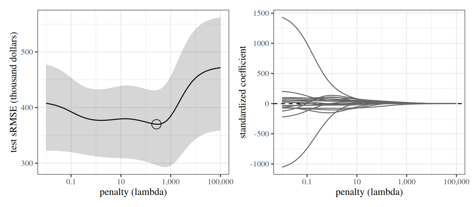
Figure 1: Ridge regression on the Hitters data. Left: test sample root mean squared error (sRMSE) against the penalty, with a shaded 95% confidence interval and the lowest value marked. Right: each standardized coefficient against the penalty, one line per predictor.
Two ggplot2 panels sharing a horizontal axis of the penalty on a logarithmic scale from 0.01 to 100000. In the left panel a shaded band marks a 95% confidence interval around the test error curve, and the test error falls as the penalty grows from the smallest values, reaches a minimum near a penalty of 300, then rises toward the error of predicting the mean for every player. In the right panel the coefficient lines spread out on the left, some positive and some negative, and all shrink smoothly toward zero as the penalty grows.
ExrExercise 6 (Predicting baseball salaries with ridge regression (part 3))

Exercise 6 (Predicting baseball salaries with ridge regression (part 3)) Use the setup of Exercise 4.

How does the test error of that \(\regpar\) compare with that of \(\regpar \approx 0\)?

Solution 6.

Show code
# Every model predicts the same test players, so differences are taken player by player.
diff_small <- mean_ci(sq_err[, 1] - sq_err[, which.min(test_mse)])
small_covers_0 <- diff_small[["lower"]] <= 0 && diff_small[["upper"]] >= 0

Almost no penalty, \(\regpar = 10^{-2}\), gives a test sRMSE of 408 ([323, 478]), which is 10% higher than the lowest. The intervals for different \(\regpar\) overlap because they use the same players, so compare errors player by player, in squared units: almost no penalty has an sMSE larger by 29,259 on average than the lowest-error penalty, with a 95% confidence interval of [-24,602, 83,119]. This interval includes 0, so on this split the improvement over almost no penalty is within what the choice of test players could produce, even though the penalty was picked because its test error was lowest.

ExrExercise 7 (Predicting baseball salaries with ridge regression (part 4))

Exercise 7 (Predicting baseball salaries with ridge regression (part 4)) Use the setup of Exercise 4.

How does the test error of that \(\regpar\) compare with that of predicting the training mean salary for every player?

Solution 7.

Show code
sq_null <- (y[-train] - mean(y[train]))^2
null_mse <- mean(sq_null)
null_rmse <- sqrt(null_mse)
diff_null <- mean_ci(sq_null - sq_err[, which.min(test_mse)])
null_covers_0 <- diff_null[["lower"]] <= 0 && diff_null[["upper"]] >= 0

Predicting the training mean salary for every player gives a test sRMSE of 474. Its sMSE is larger than that of the lowest-error penalty by 87,813 on average, with a 95% confidence interval of [24,199, 151,427]. This interval excludes 0. Both intervals reflect which players were in the test half, not which were in the training half, and both differences are optimistic for the same reason as the lowest error: the penalty was picked by looking at the test half.

ExrExercise 8 (Choose the ridge penalty by cross-validation on baseball salaries)

Exercise 8 (Choose the ridge penalty by cross-validation on baseball salaries) In Exercise 4 we chose \(\regpar\) by its error on the test half, so no player was left to estimate the error of the choice. Choose it using the training half alone instead.

Use the training half and the standardized predictors of Exercise 4. Randomly assign the training players to ten folds, and for each \(\regpar\) of that exercise’s grid compute the 10-fold cross-validation estimate and its fold-based standard error.

Solution 8. The code standardizes the predictors once on the whole training half, as in Solution 4, so the held-out fold’s means and standard deviations take part in its scaling. That leaks a little information from each held-out fold into its own fit.

x_tr <- X[train, ]
ytr <- y[train]
k_cv <- 10
set.seed(2)
fold <- sample(rep(seq_len(k_cv), length.out = length(train)))

# The squared error of each training player when its fold is held out,
# one column per penalty.
cv_sq <- sapply(lambdas, function(l) {
  sq <- numeric(length(ytr))
  for (f in seq_len(k_cv)) {
    held <- fold == f
    x_in <- x_tr[!held, ]
    b <- solve(t(x_in) %*% x_in + l * I0, t(x_in) %*% ytr[!held])
    sq[held] <- (ytr[held] - x_tr[held, ] %*% b)^2
  }
  sq
})

cv_est <- colMeans(cv_sq)
# The fold-based standard error: the standard deviation of the ten fold sMSEs over sqrt(10).
fold_mse <- apply(cv_sq, 2, function(sq) tapply(sq, fold, mean))
cv_se <- apply(fold_mse, 2, sd) / sqrt(k_cv)
import matplotlib.pyplot as plt

Xtr_py, ytr_py = X_py[train_py], y_py[train_py]
k_cv = 10
rng_cv = np.random.default_rng(2)
fold_py = rng_cv.permutation(np.arange(len(ytr_py)) % k_cv)

# The squared error of each training player when its fold is held out,
# one column per penalty.
cv_sq_py = np.empty((len(ytr_py), len(lams_py)))
for f in range(k_cv):
    held = fold_py == f
    x_in, ya = Xtr_py[~held], ytr_py[~held]
    for j, lam in enumerate(lams_py):
        b = np.linalg.solve(x_in.T @ x_in + lam * I0_py, x_in.T @ ya)
        cv_sq_py[held, j] = (ytr_py[held] - Xtr_py[held] @ b) ** 2

cv_py = cv_sq_py.mean(axis=0)
# The fold-based standard error: the standard deviation of the ten fold sMSEs over sqrt(10).
fold_mse_py = np.array([cv_sq_py[fold_py == f].mean(axis=0) for f in range(k_cv)])
se_py = fold_mse_py.std(axis=0, ddof=1) / np.sqrt(k_cv)

The numbers in the later parts of this solution are from the R split and its folds.

ExrExercise 9 (Choose the ridge penalty by cross-validation on baseball salaries (part 2))

Exercise 9 (Choose the ridge penalty by cross-validation on baseball salaries (part 2)) Use the setup of Exercise 8.

Find the \(\regpar\) with the smallest estimate, and the largest \(\regpar\) whose estimate is within one fold-based standard error of the smallest (the one-standard-error rule).

Solution 9. A ridge fit with a larger \(\regpar\) is the less flexible fit, so the one-standard-error rule picks the largest \(\regpar\) in range.

i_min <- which.min(cv_est)
i_se <- max(which(cv_est <= cv_est[i_min] + cv_se[i_min]))
picks <- c(min = i_min, one_se = i_se)

library(ggplot2)
cv_df <- data.frame(lambda = lambdas, cv = cv_est, se = cv_se)
ggplot(cv_df, aes(lambda, sqrt(cv))) +
  geom_linerange(aes(ymin = sqrt(pmax(cv - se, 0)), ymax = sqrt(cv + se)), colour = "grey60") +
  geom_line() +
  geom_point(data = cv_df[picks, ], aes(shape = names(picks)), size = 3) +
  scale_x_log10(labels = scales::label_number(big.mark = ",", drop0trailing = TRUE)) +
  scale_shape_manual(
    values = c(min = 1, one_se = 2),
    labels = c(min = "smallest estimate", one_se = "one-standard-error rule")
  ) +
  labs(x = "penalty (lambda)", y = "cross-validation RMSE (thousand dollars)", shape = NULL) +
  theme(legend.position = "bottom")
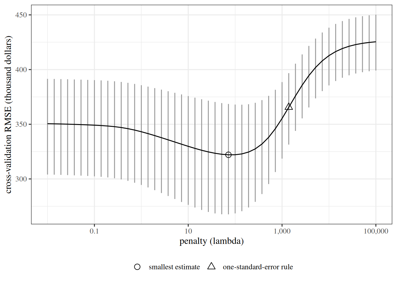
Cross-validation root mean squared error of ridge regression on the Hitters training half, against the penalty on a logarithmic scale from 0.01 to 100000, with vertical error bars of one fold-based standard error. The estimate is nearly flat for small penalties, dips to a minimum, and then climbs steeply for large penalties. Two points are marked: the minimum, and the largest penalty whose estimate lies within one standard error of the minimum, further to the right.

i_min_py = int(np.argmin(cv_py))
i_se_py = int(np.flatnonzero(cv_py <= cv_py[i_min_py] + se_py[i_min_py]).max())

fig, ax = plt.subplots(figsize=(6, 4), layout="constrained")
ax.errorbar(lams_py, np.sqrt(cv_py), color="black",
            yerr=[np.sqrt(cv_py) - np.sqrt(np.maximum(cv_py - se_py, 0)),
                  np.sqrt(cv_py + se_py) - np.sqrt(cv_py)],
            ecolor="grey");
ax.scatter(lams_py[i_min_py], np.sqrt(cv_py[i_min_py]), marker="o", s=80,
           facecolors="none", edgecolors="black", label="smallest estimate", zorder=3);
ax.scatter(lams_py[i_se_py], np.sqrt(cv_py[i_se_py]), marker="^", s=80,
           facecolors="none", edgecolors="black", label="one-standard-error rule", zorder=3);
ax.set_xscale("log");
ax.set_xlabel("penalty (lambda)");
ax.set_ylabel("cross-validation RMSE (thousand dollars)");
ax.legend();
plt.show()
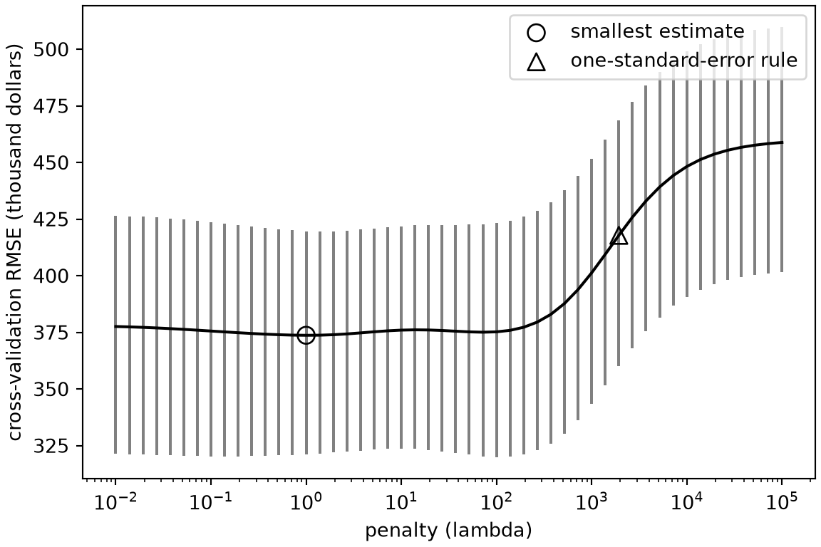
Cross-validation root mean squared error of ridge regression on the Hitters training half, against the penalty on a logarithmic scale from 0.01 to 100000, with vertical error bars of one fold-based standard error. The estimate is nearly flat for small penalties, dips to a minimum, and then climbs steeply for large penalties. Two points are marked: the minimum, and the largest penalty whose estimate lies within one standard error of the minimum, further to the right.

Each tab plots the estimates against the penalty. The smallest cross-validation estimate is at \(\regpar \approx\) 72, with a cross-validation root mean squared error (RMSE) of 322 thousand dollars. The one-standard-error rule picks the larger \(\regpar \approx\) 1389, whose estimate is 366.

ExrExercise 10 (Choose the ridge penalty by cross-validation on baseball salaries (part 3))

Exercise 10 (Choose the ridge penalty by cross-validation on baseball salaries (part 3)) Use the setup of Exercise 8.

Refit on the whole training half at each of the two penalties, and compute their test errors.

Solution 10.

test_rmse <- sapply(picks, function(i) {
  sqrt(mean((y[-train] - X[-train, ] %*% ridge(lambdas[i]))^2))
})
data.frame(
  rule = names(picks), lambda = lambdas[picks],
  cv_rmse = sqrt(cv_est[picks]), test_rmse = test_rmse
)
for name, i in [("smallest estimate", i_min_py), ("one-standard-error rule", i_se_py)]:
    b = ridge_py(lams_py[i])
    test_sq = (y_py[test_py] - X_py[test_py] @ b) ** 2
    print(name, "- lambda", round(lams_py[i]), "- cv sRMSE", round(float(np.sqrt(cv_py[i]))),
          "- test sRMSE", round(float(np.sqrt(test_sq.mean()))))
smallest estimate - lambda 1 - cv sRMSE 374 - test sRMSE 327
one-standard-error rule - lambda 1931 - cv sRMSE 418 - test sRMSE 395

The training half alone chose both penalties, so the test half gives an error estimate for each that the choice did not use. The test RMSEs are 376 at the smallest estimate and 394 at the larger penalty.

ExrExercise 11 (Choose the ridge penalty by cross-validation on baseball salaries (part 4))

Exercise 11 (Choose the ridge penalty by cross-validation on baseball salaries (part 4)) Use the setup of Exercise 8.

Do the two penalties differ much in cross-validation estimate and in test error?

Solution 11. The two penalties of Solution 9 differ by 43 in cross-validation RMSE and by 19 in test RMSE, so the larger penalty has the higher test error on this split. The rule trades a small increase in cross-validation error for a simpler, more heavily shrunken fit, and the cross-validation error alone cannot say which is better.

ReadingRead

The lab on linear models and regularization in An Introduction to Statistical Learning: With Applications in Python (ISLP for short) fits ridge regression and the lasso on these data [10, Sec. 6.5], ISLP_labs, Ch06.

4.6 Weight decay

ExrExercise 12 (What the ridge penalty does to a gradient step)

Exercise 12 (What the ridge penalty does to a gradient step) Write one gradient descent step with step size \(\learnrate\) on the ridge objective \(J_{\text{ridge}}(\vcoef) = \norm{ X\vcoef - \vy }^2 + \regpar \norm{ \vcoef }^2\), and rearrange it into the form “multiply \(\vcoef\) by a constant, then take the usual step on the loss alone”.

Solution 12. The gradient of the objective is \(\grad J_{\text{ridge}}(\vcoef) = 2\tp{X}(X\vcoef - \vy) + 2\regpar\vcoef\), so one step is

\[ \vcoef_{t} = \vcoef_{t-1} - \learnrate\,\paren{2\tp{X}(X\vcoef_{t-1} - \vy) + 2\regpar\vcoef_{t-1}} = (1 - 2\learnrate\regpar)\,\vcoef_{t-1} - 2\learnrate\,\tp{X}(X\vcoef_{t-1} - \vy). \]

The second term is the usual step on the loss alone.

ExrExercise 13 (What the ridge penalty does to a gradient step (part 2))

Exercise 13 (What the ridge penalty does to a gradient step (part 2)) Use the setup of Exercise 12.

What is the constant?

Solution 13. The penalty has become a multiplication of \(\vcoef_{t-1}\) by the constant \(1 - 2\learnrate\regpar\), which is less than \(1\) for a small enough step size, so every step first shrinks the weights toward zero.

LemTheorem 1 (A gradient step on the ridge objective is weight decay)

Theorem 1 (A gradient step on the ridge objective is weight decay) One gradient descent step with step size \(h\) on \(J_{\text{ridge}}(\vcoef) = \norm{ X\vcoef - \vy }^2 + \regpar \norm{ \vcoef }^2\) is

\[ \vcoef_{t} = (1 - 2h\regpar)\,\vcoef_{t-1} - 2h\,\tp{X}(X\vcoef_{t-1} - \vy). \]

It multiplies \(\vcoef_{t-1}\) by the constant \(1 - 2h\regpar\), then takes the usual step on the loss alone.

Proof. This is the solution to Exercise 12 and Exercise 13: see Solution 12 and Solution 13.

ExmExample 1 (One ridge step as weight decay)

Example 1 (One ridge step as weight decay) Take \(h = 0.01\), \(\regpar = 5\), \(\vcoef_{t-1} = \tp{[2, -1]}\) and a loss gradient term \(\tp{X}(X\vcoef_{t-1} - \vy) = \tp{[1, 3]}\).

Show code
wd_h <- 0.01
wd_lambda <- 5
wd_b <- c(2, -1)
wd_g <- c(1, 3)
wd_full <- wd_b - wd_h * (2 * wd_g + 2 * wd_lambda * wd_b)
wd_decay <- (1 - 2 * wd_h * wd_lambda) * wd_b - 2 * wd_h * wd_g
rbind(gradient_step = wd_full, decay_form = wd_decay)
              [,1]  [,2]
gradient_step 1.78 -0.96
decay_form    1.78 -0.96

The decay factor is \(1 - 2h\regpar = 0.9\), and both forms of Theorem 1 give the same step.

DefDefinition 1 (Weight decay)

Definition 1 (Weight decay) Weight decay shrinks the parameters by a constant factor before every gradient step, \(\vcoef_{t} = (1 - \learnrate\,\lambda_{\text{wd}})\,\vcoef_{t-1} - \learnrate\,\grad C(\vcoef_{t-1})\), where \(C\) is the loss alone and \(\lambda_{\text{wd}}\) is the decay coefficient. For plain gradient descent it is the same as an \(\lpnorm{2}\) (ridge) penalty [11]: Theorem 1 gives \(\lambda_{\text{wd}} = 2\regpar\) for the objective above.

ExmExample 2 (Weight decay reaches the ridge solution)

Example 2 (Weight decay reaches the ridge solution) In the Auto data [12], predict mpg (centered) from standardized horsepower, weight and displacement with the ridge objective \(\norm{X\vcoef - \vy}^2 + \regpar \norm{\vcoef}^2\), taking \(\regpar = 100\). Run gradient descent with weight decay for 2000 steps of size \(\learnrate = 10^{-4}\), and compare the result with the closed-form ridge solution \((\tp{X}X + \regpar I)^{-1}\tp{X}\vy\):

import numpy as np
import pandas as pd

auto_wd = pd.read_csv("data/auto.csv").dropna(subset=["horsepower"])
X_wd = auto_wd[["horsepower", "weight", "displacement"]].to_numpy(float)
X_wd = (X_wd - X_wd.mean(axis=0)) / X_wd.std(axis=0, ddof=1)
y_wd = auto_wd["mpg"].to_numpy(float)
y_wd = y_wd - y_wd.mean()

lam_wd, h_wd = 100.0, 1e-4
beta_wd = np.zeros(3)
for _ in range(2000):
    # Shrink the weights by a constant factor, then take the usual step on the loss alone.
    beta_wd = (1 - 2 * h_wd * lam_wd) * beta_wd - 2 * h_wd * X_wd.T @ (X_wd @ beta_wd - y_wd)

ridge_wd = np.linalg.solve(X_wd.T @ X_wd + lam_wd * np.eye(3), X_wd.T @ y_wd)
print(beta_wd.round(4), ridge_wd.round(4))
[-1.7301 -2.6387 -1.8075] [-1.7301 -2.6387 -1.8075]
auto_wd <- na.omit(read.csv("data/auto.csv")[, c("mpg", "horsepower", "weight", "displacement")])
X_wd <- scale(as.matrix(auto_wd[, c("horsepower", "weight", "displacement")]))
y_wd <- auto_wd$mpg - mean(auto_wd$mpg)

lam_wd <- 100
h_wd <- 1e-4
beta_wd <- rep(0, 3)
for (step in 1:2000) {
  # Shrink the weights by a constant factor, then take the usual step on the loss alone.
  beta_wd <- (1 - 2 * h_wd * lam_wd) * beta_wd - 2 * h_wd * drop(t(X_wd) %*% (X_wd %*% beta_wd - y_wd))
}

ridge_wd <- solve(crossprod(X_wd) + lam_wd * diag(3), crossprod(X_wd, y_wd))
rbind(weight_decay = round(beta_wd, 4), closed_form = round(drop(ridge_wd), 4))
             horsepower  weight displacement
weight_decay    -1.7301 -2.6387      -1.8075
closed_form     -1.7301 -2.6387      -1.8075

The two routes agree to 1.2e-14, as the definition says they must for plain gradient descent. Each step multiplies the weights by \(1 - 2\learnrate\regpar =\) 0.98 before the usual loss step, so the weights are pulled toward zero throughout, not only at the end.

Deep learning libraries expose weight decay as an option of the optimizer, and its coefficient can differ from the penalty’s \(\regpar\) by a constant such as this \(2\), depending on how the loss is scaled, so compare definitions before reusing a value. Some papers write the decay as a rate per step instead, \(\vcoef_{t} = (1 - \lambda)\,\vcoef_{t-1} - \learnrate\,\grad C(\vcoef_{t-1})\) [13], whose \(\lambda\) equals \(\learnrate\,\lambda_{\text{wd}}\) and so moves with the step size. The equivalence with a penalty holds for plain gradient descent only. Under an adaptive method such as Adam (see Gradient Descent), a penalty’s gradient is divided by the adaptive denominator along with the loss gradient, so the shrinkage differs from coordinate to coordinate; decoupled weight decay, as in AdamW [13], applies the shrinkage directly. Libraries offer both, so check which one an optimizer’s weight decay option means.

5 The lasso

The lasso — Tibshirani [14] — adds a penalty on the \(\ell_1\) norm of \(\vcoef\) instead:

\[\argmin_{\vcoef} (y - X\vcoef)^T (y - X\vcoef) + \regpar\norm{\vcoef}_1\]

or, written out,

\[\min_{\vcoef} \sumin \paren{\dprod{\vx_i}{\vcoef} - y_i}^2 + \regpar\paren{|\coef{1}| + \dots + |\coef{d}|}\]

  • Unlike ridge, which has the closed-form solution Equation 2, the lasso has none; fitting it is a quadratic programming problem.

  • It promotes sparsity in \(\vcoef\), favoring solutions with many \(\coef{i} = 0\). As a byproduct, it sub-selects the features of the input that are important.

  • The constraint \(\norm{\vcoef}_1 \leq t\) defines a region, a diamond in two dimensions with its corners on the axes. \(\regpar\) sets how tight that constraint is. The solution tends to land at a corner, and a corner is a \(\vcoef\) with some coordinates equal to zero.

We would really like to penalize the number of non-zero coefficients. That count is not convex — it jumps as a coefficient crosses zero rather than sloping — so gradient-based methods cannot minimize it. The \(\ell_1\) penalty approximates it, because \(q = 1\) is the smallest exponent for which \(\norm{\vcoef}_q\) is convex. That makes it the closest convex relaxation of the count.

The \(\ell_1\) penalty corresponds to a Laplace distribution prior, which is not differentiable at zero.
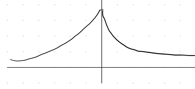
Hand-drawn density curve of the Laplace distribution, with a sharp point at zero on the vertical axis and tails that fall away on both sides toward the horizontal axis

ExrExercise 14 (Fit a constant with squared and absolute loss)

Exercise 14 (Fit a constant with squared and absolute loss) Five responses are \(1\), \(2\), \(4\), \(9\) and \(100\). Find the single constant \(c\) that minimizes the sum of squared deviations, and the constant that minimizes the sum of absolute deviations.

Solution 14. Squared deviations. The minimizer is the mean, \((1 + 2 + 4 + 9 + 100)/5 = 23.2\). The outlier \(100\) pulls the fit far from the other four points.

Absolute deviations. The minimizer is the median, \(4\). Moving \(c\) slightly changes the sum by one unit per response on each side. The loss falls when more responses lie on the side \(c\) moves toward. So the minimum sits where half the responses are on each side. The outlier barely moves the fit.

ExrExercise 15 (Fit a constant with squared and absolute loss (part 2))

Exercise 15 (Fit a constant with squared and absolute loss (part 2)) Use the setup of Exercise 14.

At each minimizer, how many of the five residuals are exactly zero?

Solution 15. At the squared-loss minimizer, no response equals \(23.2\), so no residual is zero. At the absolute-loss minimizer, the residuals are \(-3\), \(-2\), \(0\), \(5\) and \(96\), so exactly one is zero.

ExrExercise 16 (Fit a constant with squared and absolute loss (part 3))

Exercise 16 (Fit a constant with squared and absolute loss (part 3)) Use the setup of Exercise 14.

How does this compare with the lasso’s exact zeros?

Solution 16. Comparison with the lasso. The absolute value has a kink at \(0\), so the loss is not smooth where a residual is zero, and the minimizer can sit exactly on the kink. The lasso penalty \(\abs{\coef{j}}\) has the same kink, so it sets coefficients exactly to zero. Squared loss and the ridge penalty are smooth at zero, so they push values toward zero without landing on it. By analogy, absolute loss tends to produce sparse residuals: a fit that matches some responses exactly and ignores how far off the rest are.

VideosWatch
ReadingRead

GeeksforGeeks explains lasso regression [16].

5.1 Solving the lasso by coordinate descent

The lasso has no closed-form solution, but it has a simple iterative solution. Gradient descent does not apply directly, because the \(\ell_1\) penalty is not differentiable at zero. Coordinate descent sidesteps that by updating one coefficient at a time. It holds the other \(d - 1\) coefficients fixed, and minimizes the objective exactly over the one that is free. Each such one-dimensional problem has a closed-form solution, and its solution shows where the lasso’s zeros come from.

DefDefinition 2 (The soft-thresholding operator)

Definition 2 (The soft-thresholding operator) For \(z \in \reals\) and \(\tau \ge 0\), the soft-thresholding operator is \[ S_\tau(z) = \begin{cases} z - \tau & \text{if } z > \tau \\ 0 & \text{if } -\tau \le z \le \tau \\ z + \tau & \text{if } z < -\tau. \end{cases} \] It shrinks \(z\) toward zero by \(\tau\), and sets it to exactly zero when \(|z| \le \tau\). Equivalently, \(S_\tau(z) = \sign(z)\,\max(|z| - \tau,\, 0)\) [17].

ExmExample 3 (Soft-thresholding at \(\tau = 1\))

Example 3 (Soft-thresholding at \(\tau = 1\)) \(S_1(3) = 2\), because \(3 > 1\) and \(3 - 1 = 2\). \(S_1(\tfrac12) = 0\), because \(|\tfrac12| \le 1\). \(S_1(-\tfrac52) = -\tfrac32\), because \(-\tfrac52 < -1\) and \(-\tfrac52 + 1 = -\tfrac32\).

DefDefinition 3 (Cyclic coordinate descent)

Definition 3 (Cyclic coordinate descent) Write \(X_{\cdot j}\) for the \(j\)th column of \(X\). Cyclic coordinate descent cycles through the coordinates \(j = 1, \dots, d\). At each, it replaces \(\coef{j}\) by the minimizer of the objective over \(\coef{j}\) alone, with the other coefficients held fixed. Let \(r_j = y - \sum_{k \ne j} X_{\cdot k}\coef{k}\) be the partial residual. For the lasso, that minimizer is \(\coef{j} = S_{\regpar/2}\paren{\dprod{X_{\cdot j}}{r_j}}/\norm{X_{\cdot j}}^2\), which Exercise 18 asks you to derive. One pass through all \(d\) coordinates is a sweep, and sweeps repeat until the coefficients stop changing.

ExmExample 4 (One sweep, by hand)

Example 4 (One sweep, by hand) Take \(d = 2\) with orthogonal columns, \(X_{\cdot 1}^T X_{\cdot 2} = 0\), so that \(\dprod{X_{\cdot 1}}{r_1}\) does not depend on \(\coef{2}\), and the reverse. Starting from \(\coef{1} = \coef{2} = 0\), the first update sets \(\coef{1} = S_{\regpar/2}\paren{\dprod{X_{\cdot 1}}{y}}/\norm{X_{\cdot 1}}^2\). The second sets \(\coef{2} = S_{\regpar/2}\paren{\dprod{X_{\cdot 2}}{y}}/\norm{X_{\cdot 2}}^2\), because \(r_2 = y - X_{\cdot 1}\coef{1}\) and \(\dprod{X_{\cdot 2}}{X_{\cdot 1}} = 0\). A second sweep changes nothing. With orthogonal columns, one sweep therefore solves the lasso, and each coefficient is a soft-thresholded least squares coefficient.

Coordinate descent converges to a global minimizer of the lasso objective. The squared error is smooth and convex, and the \(\ell_1\) penalty is convex and a sum of terms that each involve one coordinate, which are the conditions that guarantee convergence for coordinate descent [18].

ExrExercise 17 (The coordinate update for the lasso)

Exercise 17 (The coordinate update for the lasso) Take all the parameters except the coefficient \(\coef{j}\) of feature \(j\) as given. Let \(r_j = y - \sum_{k \ne j} X_{\cdot k}\coef{k}\) be the partial residual, the part of \(y\) that the other \(d - 1\) features leave unexplained. The lasso objective, as a function of \(\coef{j}\) alone, is \[ f(\coef{j}) = \norm{r_j - X_{\cdot j}\coef{j}}^2 + \regpar\,|\coef{j}|. \]

Show that \(f(\coef{j}) = \norm{X_{\cdot j}}^2\coef{j}^2 - 2\,\dprod{X_{\cdot j}}{r_j}\,\coef{j} + \regpar\,|\coef{j}| + \text{constant}\).

Solution 17. Expand the square: \[ \norm{r_j - X_{\cdot j}\coef{j}}^2 = \norm{r_j}^2 - 2\,\dprod{X_{\cdot j}}{r_j}\,\coef{j} + \norm{X_{\cdot j}}^2\coef{j}^2. \] The first term does not depend on \(\coef{j}\), so it is the constant.

ExrExercise 18 (The coordinate update for the lasso (part 2))

Exercise 18 (The coordinate update for the lasso (part 2)) Use the setup of Exercise 17.

Show that the minimizer is \[ \coef{j} = \frac{S_{\regpar/2}\paren{\dprod{X_{\cdot j}}{r_j}}}{\norm{X_{\cdot j}}^2}, \] where \(S_\tau\) is the soft-thresholding operator. Hint: treat \(\coef{j} > 0\), \(\coef{j} < 0\) and \(\coef{j} = 0\) separately. On the first two, \(f\) is differentiable.

Solution 18. Write \(a = \norm{X_{\cdot j}}^2\), which is positive because the column is not the zero vector, and \(c = \dprod{X_{\cdot j}}{r_j}\), so that \(f(\coef{j}) = a\coef{j}^2 - 2c\,\coef{j} + \regpar\,|\coef{j}| + \text{constant}\). - For \(\coef{j} > 0\), \(f'(\coef{j}) = 2a\coef{j} - 2c + \regpar\), which is zero at \(\coef{j} = (c - \regpar/2)/a\). That is positive, so it is a valid solution, exactly when \(c > \regpar/2\). - For \(\coef{j} < 0\), \(f'(\coef{j}) = 2a\coef{j} - 2c - \regpar\), which is zero at \(\coef{j} = (c + \regpar/2)/a\). That is negative exactly when \(c < -\regpar/2\). - Otherwise, \(|c| \le \regpar/2\). Then \(f'(\coef{j}) = 2a\coef{j} - 2c + \regpar > 0\) for every \(\coef{j} > 0\), because \(2a\coef{j} > 0\) and \(-2c + \regpar \ge 0\). Likewise \(f'(\coef{j}) < 0\) for every \(\coef{j} < 0\). So \(f\) falls until zero and rises after it, and its minimizer is \(\coef{j} = 0\).

Together, these three cases say \(\coef{j} = S_{\regpar/2}(c)/a\).

ExrExercise 19 (The coordinate update for the lasso (part 3))

Exercise 19 (The coordinate update for the lasso (part 3)) Use the setup of Exercise 17.

For which values of \(\dprod{X_{\cdot j}}{r_j}\) is the minimizer exactly zero?

Solution 19. The minimizer of Solution 18 is exactly zero when \(|\dprod{X_{\cdot j}}{r_j}| \le \regpar/2\).

ExrExercise 20 (The coordinate update for the lasso (part 4))

Exercise 20 (The coordinate update for the lasso (part 4)) Use the setup of Exercise 17.

What does that say about a feature that is only weakly correlated with the residual?

Solution 20. A feature whose inner product with the residual is small cannot reduce the squared error by enough to outweigh the penalty on its coefficient, so the lasso leaves it out. So the lasso selects features. Ridge regression never does: its penalty \(\regpar\coef{j}^2\) has slope zero at zero, so any non-zero inner product pulls the coefficient off zero.

ExrExercise 21 (The coordinate update for the lasso (part 5))

Exercise 21 (The coordinate update for the lasso (part 5)) Use the setup of Exercise 17.

Set \(\regpar = 0\). What does the update reduce to?

Solution 21. With \(\regpar = 0\), \(S_0(c) = c\), and the update is \(\coef{j} = \dprod{X_{\cdot j}}{r_j}/\norm{X_{\cdot j}}^2\). That is the least squares coefficient of the residual \(r_j\) on the single feature \(X_{\cdot j}\). Coordinate descent then amounts to fitting each feature to what the others leave unexplained, in turn.

Now apply it. We use the same training half and standardized predictors as Exercise 4. We center the salaries on the training mean, which takes care of the intercept.

# Soft-thresholding shrinks z toward zero by tau,
# and returns exactly zero when |z| <= tau, which makes the lasso sparse.
def soft_py(z, tau):
  return np.sign(z) * max(abs(z) - tau, 0.0)

def lasso_cd_py(X, y, lam, tol=1e-8, max_sweeps=5000):
  beta = np.zeros(X.shape[1])
  col_ss = (X**2).sum(axis=0)  # ||X_j||^2 for each column, which does not change
  for _ in range(max_sweeps):
      biggest_change = 0.0
      for j in range(X.shape[1]):
          # Partial residual: y minus every feature's contribution except feature j's.
          r_j = y - X @ beta + X[:, j] * beta[j]
          new = soft_py(X[:, j] @ r_j, lam / 2) / col_ss[j]
          biggest_change = max(biggest_change, abs(new - beta[j]))
          beta[j] = new
      # Stop once a full sweep barely moves any coefficient.
      if biggest_change < tol:
          break
  return beta

# Drop the intercept column of X_py; centering y takes care of the intercept.
Xtr_py = X_py[train_py, 1:]
ytr_py = y_py[train_py] - y_py[train_py].mean()
lam_max_py = 2 * np.abs(Xtr_py.T @ ytr_py).max()  # the smallest lambda that zeroes every coefficient
lams_lasso_py = lam_max_py * 10.0 ** np.linspace(-4, 0, 30)

nonzero_py, mse_lasso_py = [], []
for lam in lams_lasso_py:
  b = lasso_cd_py(Xtr_py, ytr_py, lam)
  nonzero_py.append(int((b != 0).sum()))
  pred = y_py[train_py].mean() + X_py[test_py, 1:] @ b
  mse_lasso_py.append(np.mean((y_py[test_py] - pred) ** 2))
print("nonzero coefficients at the smallest and largest lambda:", nonzero_py[0], nonzero_py[-1])
nonzero coefficients at the smallest and largest lambda: 19 0
print("lowest test MSE:", round(min(mse_lasso_py)), "with", nonzero_py[int(np.argmin(mse_lasso_py))], "nonzero coefficients")
lowest test MSE: 106793 with 14 nonzero coefficients
# Soft-thresholding shrinks z toward zero by tau,
# and returns exactly zero when |z| <= tau, which makes the lasso sparse.
soft <- function(z, tau) sign(z) * pmax(abs(z) - tau, 0)

lasso_cd <- function(x_mat, y, lambda, tol = 1e-8, max_sweeps = 5000) {
beta <- rep(0, ncol(x_mat))
col_ss <- colSums(x_mat^2) # ||X_j||^2 for each column, which does not change
for (s in seq_len(max_sweeps)) {
  biggest_change <- 0
  for (j in seq_len(ncol(x_mat))) {
    # Partial residual: y minus every feature's contribution except j's.
    r_j <- y - x_mat %*% beta + x_mat[, j] * beta[j]
    new <- soft(sum(x_mat[, j] * r_j), lambda / 2) / col_ss[j]
    biggest_change <- max(biggest_change, abs(new - beta[j]))
    beta[j] <- new
  }
  # Stop once a full sweep barely moves any coefficient.
  if (biggest_change < tol) break
}
beta
}

# Drop the intercept column of x_mat; centering y takes care of the intercept.
x_train <- Xs[train, ]
ytr <- y[train] - mean(y[train])
# The smallest lambda that zeroes every coefficient.
lambda_max <- 2 * max(abs(crossprod(x_train, ytr)))
lambdas_lasso <- lambda_max * 10^seq(-4, 0, length.out = 30)

fits <- sapply(lambdas_lasso, function(l) lasso_cd(x_train, ytr, l))
nonzero <- colSums(fits != 0)
mse_lasso <- apply(
fits, 2,
function(b) mean((y[-train] - mean(y[train]) - Xs[-train, ] %*% b)^2)
)
print(nonzero[c(1, 30)])
[1] 19  0
best <- which.min(mse_lasso)
c(lowest_mse = min(mse_lasso), nonzero_at_lowest = unname(nonzero[best]))
       lowest_mse nonzero_at_lowest 
         141389.5               9.0 
Show code
# At a solution, the gradient of the squared error balances the penalty's slope:
# 2 X_j'(y - Xb) = lambda * sign(b_j) when b_j is not zero,
# and |2 X_j'(y - Xb)| <= lambda when b_j is zero.
i_mid <- 15
b_mid <- fits[, i_mid]
score <- 2 * crossprod(x_train, ytr - x_train %*% b_mid)
kkt_gap <- max(
abs(score[b_mid != 0] - lambdas_lasso[i_mid] * sign(b_mid[b_mid != 0])),
pmax(abs(score[b_mid == 0]) - lambdas_lasso[i_mid], 0)
)
stopifnot(kkt_gap < 1e-5)
fmt <- function(x) format(round(x), big.mark = ",", scientific = FALSE)

The two languages split the players at random in different ways, so their numbers differ. The numbers below are from the R split.

With the smallest \(\regpar\) in the grid, all 19 coefficients are non-zero. With the largest, 0 are. The lowest test error, 141,389, comes with 9 non-zero coefficients. For comparison, ridge regression reached 136,857 in Solution 5, but it keeps every predictor.

As a check that coordinate descent has found the minimizer, the lasso’s optimality conditions hold at the middle \(\regpar\) in the grid to within \(10^{-5}\). The three cases of Solution 18 encode these conditions: the penalty’s slope \(\regpar\,\sign(\coef{j})\) balances the gradient of the squared error for each non-zero coefficient, and the gradient is no larger than \(\regpar\) in absolute value for each zero one.

LemTheorem 2 (The coordinate update for the lasso)

Theorem 2 (The coordinate update for the lasso) Let \(\regpar \ge 0\) and suppose the column \(X_{\cdot j}\) is not the zero vector, so that \(\norm{X_{\cdot j}}^2 > 0\). Take all the parameters except the coefficient \(\coef{j}\) of feature \(j\) as given, and let \(r_j = y - \sum_{k \ne j} X_{\cdot k}\coef{k}\) be the partial residual. The minimizer of \(f(\coef{j}) = \norm{r_j - X_{\cdot j}\coef{j}}^2 + \regpar\,|\coef{j}|\) is

\[ \coef{j} = \frac{S_{\regpar/2}\paren{\dprod{X_{\cdot j}}{r_j}}}{\norm{X_{\cdot j}}^2}, \]

where \(S_\tau\) is the soft-thresholding operator of Definition 2. It is exactly zero when \(\abs{\dprod{X_{\cdot j}}{r_j}} \le \regpar/2\).

Proof. This is the solution to Exercise 18 and Exercise 19: see Solution 18 and Solution 19.

ReadingRead

Friedman, Hastie and Tibshirani describe the coordinate descent algorithm behind the glmnet package [19].

ExrExercise 22 (Shrink the least squares coefficients with ridge and the lasso)

Exercise 22 (Shrink the least squares coefficients with ridge and the lasso) Let \(X\) be an \(n \times \ninputvars\) matrix whose columns are orthonormal, so that \(\tp{X}X = I_{\ninputvars}\), and let \(\vy \in \reals^n\). There is no intercept. Write \(\hcoef{j}\) for the least squares coefficient of feature \(j\).

Express the \(j\)th coefficient of the ridge fit as a function of \(\hcoef{j}\) and \(\regpar\).

Solution 22. The least squares coefficients solve the normal equations \(\tp{X}X\vcoef = \tp{X}\vy\), and \(\tp{X}X = I_{\ninputvars}\), so \(\hcoef{j} = \dprod{X_{\cdot j}}{\vy}\).

Ridge. The closed-form solution Equation 2, without an intercept, is \(\paren{\tp{X}X + \regpar I_{\ninputvars}}^{-1}\tp{X}\vy\). Here \(\tp{X}X + \regpar I_{\ninputvars} = (1 + \regpar) I_{\ninputvars}\), so the \(j\)th coefficient is \[\frac{\hcoef{j}}{1 + \regpar}.\]

ExrExercise 23 (Shrink the least squares coefficients with ridge and the lasso (part 2))

Exercise 23 (Shrink the least squares coefficients with ridge and the lasso (part 2)) Use the setup of Exercise 22.

Express the \(j\)th coefficient of the lasso fit as a function of \(\hcoef{j}\) and \(\regpar\).

Solution 23. The lasso. With orthonormal columns, the squared error separates into one term per coefficient: \(\norm{X\vcoef - \vy}^2 = \sum_{j=1}^{\ninputvars} \paren{\coef{j} - \hcoef{j}}^2 + \text{a constant that does not involve } \vcoef\), so the lasso objective is a sum of one-coefficient problems. Each one is the problem of Theorem 2 with a single observation, \(X_{\cdot j} = 1\) and \(r_j = \hcoef{j}\). Its minimizer is \(S_{\regpar/2}\paren{\hcoef{j}}\), the soft-thresholded coefficient of Definition 2.

ExrExercise 24 (Shrink the least squares coefficients with ridge and the lasso (part 3))

Exercise 24 (Shrink the least squares coefficients with ridge and the lasso (part 3)) Use the setup of Exercise 22.

How does each method change \(\hcoef{j}\)?

Solution 24. Ridge divides every least squares coefficient by the same number, \(1 + \regpar\). Each coefficient keeps its sign, and none becomes exactly zero.

The lasso subtracts the same amount, \(\regpar/2\), from the size of every least squares coefficient, and sets a coefficient to exactly zero when its size is at most \(\regpar/2\).

LemTheorem 3 (Ridge and the lasso with orthonormal features)

Theorem 3 (Ridge and the lasso with orthonormal features) Let \(X\) be an \(n \times \ninputvars\) matrix with \(\tp{X}X = I_{\ninputvars}\), let \(\vy \in \reals^n\) and let \(\regpar \ge 0\). Let \(\hcoef{j} = \dprod{X_{\cdot j}}{\vy}\). Then the \(j\)th coefficient of the minimizer of \(\norm{X\vcoef - \vy}^2 + \regpar\norm{\vcoef}^2\) is

\[ \frac{\hcoef{j}}{1 + \regpar}, \]

and the \(j\)th coefficient of the minimizer of \(\norm{X\vcoef - \vy}^2 + \regpar\norm{\vcoef}_1\) is \(S_{\regpar/2}\paren{\hcoef{j}}\), where \(S_\tau\) is the soft-thresholding operator.

Proof. This is the answer to Exercise 22, Exercise 23 and Exercise 24: see Solution 22, Solution 23 and Solution 24.

ExmExample 5 (Five least squares coefficients shrunk at \(\regpar = 2\))

Example 5 (Five least squares coefficients shrunk at \(\regpar = 2\)) Take \(X = I_5\), the identity matrix, so that the columns are orthonormal and \(\hcoef{j} = y_j\). Let \(\vy = \tp{[3, 1.2, 0.3, -0.8, -2.5]}\) and \(\regpar = 2\).

Show code
oo_y <- c(3, 1.2, 0.3, -0.8, -2.5)
oo_lambda <- 2
oo_soft <- function(z, tau) sign(z) * pmax(abs(z) - tau, 0)
oo_ridge <- drop(solve(diag(5) + oo_lambda * diag(5), oo_y))
oo_lasso <- oo_soft(oo_y, oo_lambda / 2)
rbind(least_squares = oo_y, ridge = oo_ridge, lasso = oo_lasso)
              [,1] [,2] [,3]       [,4]       [,5]
least_squares    3  1.2  0.3 -0.8000000 -2.5000000
ridge            1  0.4  0.1 -0.2666667 -0.8333333
lasso            2  0.2  0.0  0.0000000 -1.5000000

Ridge divides each coefficient by \(1 + \regpar = 3\), so \(3\) becomes \(1\) and \(0.3\) becomes \(0.1\). The lasso subtracts \(\regpar/2 = 1\) from the size of each coefficient: \(3\) becomes \(2\), \(1.2\) becomes \(0.2\) and \(-2.5\) becomes \(-1.5\). The coefficients \(0.3\) and \(-0.8\), which are no larger than \(1\) in size, become exactly zero.

Show code
library(ggplot2)
shrink <- data.frame(ls = seq(-4, 4, length.out = 401))
shrink$ridge <- shrink$ls / (1 + oo_lambda)
shrink$lasso <- oo_soft(shrink$ls, oo_lambda / 2)
shrink_long <- rbind(
  data.frame(ls = shrink$ls, estimate = shrink$ridge, method = "ridge"),
  data.frame(ls = shrink$ls, estimate = shrink$lasso, method = "lasso")
)
ggplot(shrink_long) +
  aes(ls, estimate, colour = method) +
  geom_abline(slope = 1, intercept = 0, linetype = "dashed", colour = "grey50") +
  geom_line() +
  coord_equal() +
  labs(x = "least squares coefficient", y = "penalized coefficient", colour = NULL)
Show code
import matplotlib.pyplot as plt
import numpy as np

lam = 2.0
ls = np.linspace(-4, 4, 401)
ridge = ls / (1 + lam)
lasso = np.sign(ls) * np.maximum(np.abs(ls) - lam / 2, 0)

fig, ax = plt.subplots(figsize=(5, 3.5), layout="constrained")
ax.plot(ls, ls, "--", color="grey", label="least squares");
ax.plot(ls, ridge, label="ridge");
ax.plot(ls, lasso, label="lasso");
ax.set_aspect("equal");
ax.set_xlabel("least squares coefficient");
ax.set_ylabel("penalized coefficient");
ax.legend();
plt.show()
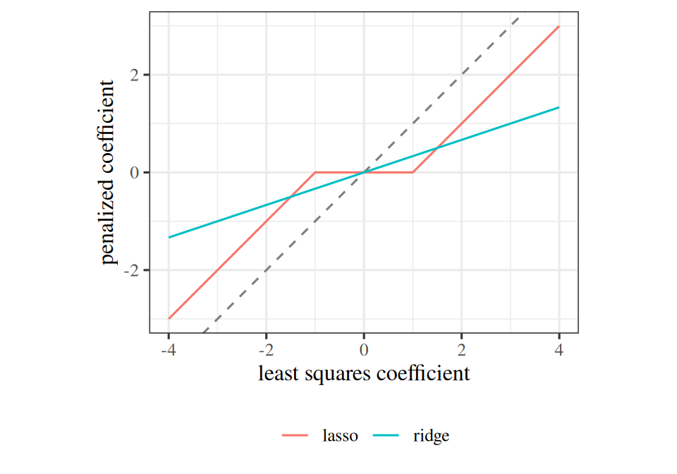
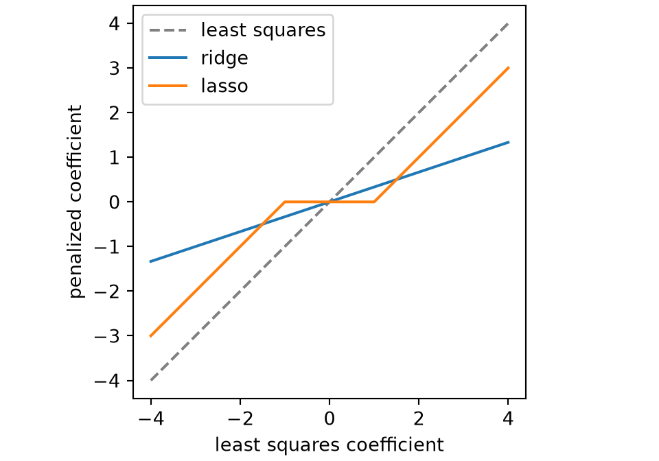
Figure 2: Ridge and the lasso shrink the least squares coefficients in the orthonormal case, with \(\regpar = 2\). Ridge shrinks every coefficient by the same proportion. The lasso shrinks every coefficient by the same amount, and sets the small ones to zero.
(a)
Line graph with the least squares coefficient on the horizontal axis and the penalized coefficient on the vertical axis, both from -4 to 4. A dashed diagonal line shows least squares, with no penalty. The ridge line is a straight line through the origin with a smaller slope, one third. The lasso line is flat at zero between -1 and 1, then rises with slope 1, parallel to the dashed line and shifted toward zero by 1.
(b)
Line graph with the least squares coefficient on the horizontal axis and the penalized coefficient on the vertical axis, both from -4 to 4. A dashed diagonal line shows least squares, with no penalty. The ridge line is a straight line through the origin with a smaller slope, one third. The lasso line is flat at zero between -1 and 1, then rises with slope 1, parallel to the dashed line and shifted toward zero by 1.
ExrExercise 25 (Predict how ridge and lasso coefficients differ)

Exercise 25 (Predict how ridge and lasso coefficients differ) You fit ridge regression and the lasso to the same data, and increase \(\regpar\) from \(0\) to very large. Predict what happens to the fitted coefficients in each case.

Solution 25. Ridge. Every coefficient shrinks smoothly toward zero as \(\regpar\) grows.

Lasso. The lasso sets coefficients to exactly zero, one feature at a time. So the features least related to the response drop out first, and the last survivors are the strongest. For large enough \(\regpar\) every lasso coefficient is zero; the ridge coefficients are only small.

ExrExercise 26 (Predict how ridge and lasso coefficients differ (part 2))

Exercise 26 (Predict how ridge and lasso coefficients differ (part 2)) Use the setup of Exercise 25.

In particular, when will a coefficient be exactly zero?

Solution 26. Ridge. No coefficient is ever exactly zero for a finite \(\regpar\). The penalty \(\regpar\norm{\vcoef}_2^2\) has a gradient that goes to zero with the coefficient, so a small coefficient feels almost no push and settles near zero without reaching it.

Lasso. The penalty \(\regpar\norm{\vcoef}_1\) pushes with the same force \(\regpar\) however small the coefficient is, and that push beats the data’s pull when the feature is only weakly related to the residual. By Theorem 2, a coefficient is zero exactly when \(\abs{\dprod{X_{\cdot j}}{r_j}} \leq \regpar/2\). Geometrically, the diamond-shaped constraint region has corners on the axes, and the solution tends to land on a corner.

ExrExercise 27 (Draw where the constrained fit lands)

Exercise 27 (Draw where the constrained fit lands) Two features are positively correlated, so the squared error of a fit with coefficients \(\vcoef = (\coef{1}, \coef{2})\) is

\[ J(\vcoef) = d_1^2 + 1.6\, d_1 d_2 + d_2^2, \qquad d_j = \coef{j} - \hcoef{j}, \]

with least-squares fit \(\hat{\vcoef} = (1.5, 0.1)\). Constrain the fit to the diamond \(\abs{\coef{1}} + \abs{\coef{2}} \leq 1\) (the L1 ball), then to the disc \(\coef{1}^2 + \coef{2}^2 \leq 1\) (the L2 ball).

Sketch the level sets of \(J\), and the two constraint regions.

Solution 27. The level sets of \(J\) are ellipses around \(\hat{\vcoef}\), tilted because the features are correlated. The unconstrained minimum lies outside both regions, so the best constrained point is where the smallest ellipse that reaches a region first touches its boundary.

ExrExercise 28 (Draw where the constrained fit lands (part 2))

Exercise 28 (Draw where the constrained fit lands (part 2)) Use the setup of Exercise 27.

Predict where on each region’s boundary the lowest level set of \(J\) first touches it.

Solution 28. A smooth boundary, like the disc’s, is touched at a point where the ellipse and the circle are tangent, which is generally not on an axis. The diamond has corners on the axes, and an ellipse sweeping in from outside reaches a corner first whenever the ellipse’s tilt does not line up with an edge.

ExrExercise 29 (Draw where the constrained fit lands (part 3))

Exercise 29 (Draw where the constrained fit lands (part 3)) Use the setup of Exercise 27.

Which fit has a coefficient that is exactly zero?

Solution 29. With these numbers the ellipse’s tilt does not line up with an edge, so it reaches a corner of the diamond first, and the diamond’s fit has a coefficient that is exactly zero. The disc’s fit has none. With other numbers the ellipse can touch an edge instead, and then the best point has no zero coefficient.

ExrExercise 30 (Draw where the constrained fit lands (part 4))

Exercise 30 (Draw where the constrained fit lands (part 4)) Use the setup of Exercise 27.

Check your prediction by computing the best point inside each region.

Solution 30. The code searches a fine grid of coefficient pairs for the lowest \(J\) that satisfies each constraint.

Show code
library(ggplot2)

# The squared error J on a fine grid of (b1, b2), with the least-squares
# fit (1.5, 0.1) from the exercise.
grid <- expand.grid(
  b1 = seq(-2, 2, length.out = 801),
  b2 = seq(-2, 2, length.out = 801)
)
d1 <- grid$b1 - 1.5
d2 <- grid$b2 - 0.1
grid$J <- d1^2 + 1.6 * d1 * d2 + d2^2
grid$l1 <- abs(grid$b1) + abs(grid$b2)
grid$l2 <- sqrt(grid$b1^2 + grid$b2^2)

# The best point inside each region: the lowest J among the grid points that
# satisfy the constraint.
inside_l1 <- subset(grid, l1 <= 1 + 1e-9)
inside_l2 <- subset(grid, l2 <= 1 + 1e-9)
best <- rbind(
  cbind(inside_l1[which.min(inside_l1$J), c("b1", "b2")], penalty = "L1"),
  cbind(inside_l2[which.min(inside_l2$J), c("b1", "b2")], penalty = "L2")
)
best
Show code
ggplot(grid) +
  aes(b1, b2) +
  geom_contour(aes(z = J), breaks = c(0.1, 0.3, 0.6, 1, 1.5), colour = "grey60") +
  geom_contour(aes(z = l1), breaks = 1, colour = "#0072B2") +
  geom_contour(aes(z = l2), breaks = 1, colour = "#D55E00") +
  geom_point(aes(shape = penalty, colour = penalty), data = best, size = 3) +
  scale_colour_manual(values = c(L1 = "#0072B2", L2 = "#D55E00")) +
  coord_fixed(xlim = c(-1.5, 2), ylim = c(-1.5, 1.5)) +
  labs(
    x = expression("First coefficient, " * beta[1]),
    y = expression("Second coefficient, " * beta[2]),
    colour = NULL, shape = NULL
  ) +
  theme(legend.position = "bottom")
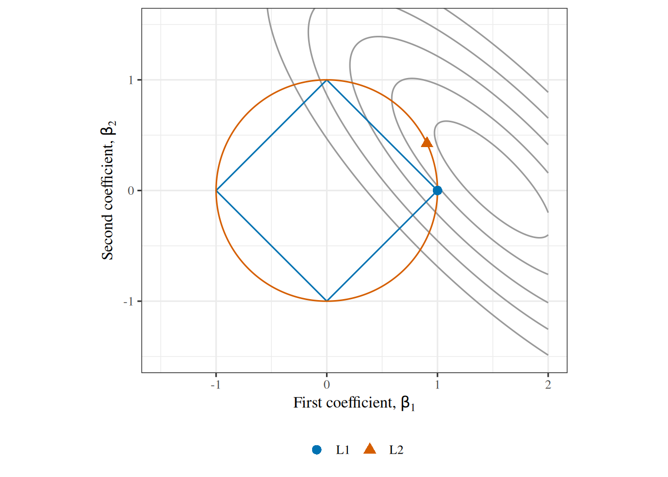
Elliptical contour lines of the squared error, tilted so that they run from upper left to lower right, centred on the least-squares point (1.5, 0.1) outside both regions. A diamond with corners at (+-1, 0) and (0, +-1) and a circle of radius 1 are drawn around the origin. A point marks the best fit inside each region: it sits on the diamond's right corner, (1, 0), and on the circle at about (0.91, 0.43).

Show code
import matplotlib.pyplot as plt
import numpy as np

# The squared error J on a fine grid of (b1, b2), with the least-squares
# fit (1.5, 0.1) from the exercise.
b = np.linspace(-2, 2, 801)
b1, b2 = np.meshgrid(b, b)
d1 = b1 - 1.5
d2 = b2 - 0.1
J = d1**2 + 1.6 * d1 * d2 + d2**2
l1 = np.abs(b1) + np.abs(b2)
l2 = np.sqrt(b1**2 + b2**2)

# The best point inside each region: the lowest J among the grid points that
# satisfy the constraint (np.inf hides the others from argmin).
best = {}
for name, norm in [("L1", l1), ("L2", l2)]:
    k = np.argmin(np.where(norm <= 1 + 1e-9, J, np.inf))
    best[name] = (b1.flat[k], b2.flat[k])
print(best)
{'L1': (np.float64(1.0), np.float64(0.0)), 'L2': (np.float64(0.9050000000000002), np.float64(0.42500000000000027))}
Show code
fig, ax = plt.subplots(figsize=(6, 4.5), layout="constrained")
ax.contour(b1, b2, J, levels=[0.1, 0.3, 0.6, 1, 1.5], colors="grey");
ax.contour(b1, b2, l1, levels=[1], colors="#0072B2");
ax.contour(b1, b2, l2, levels=[1], colors="#D55E00");
ax.scatter(*best["L1"], marker="o", c="#0072B2", label="L1");
ax.scatter(*best["L2"], marker="^", c="#D55E00", label="L2");
ax.set_xlim(-1.5, 2);
ax.set_ylim(-1.5, 1.5);
ax.set_aspect("equal");
ax.set_xlabel(r"First coefficient, $\beta_1$");
ax.set_ylabel(r"Second coefficient, $\beta_2$");
fig.legend(loc="outside lower center", ncol=2);
plt.show()
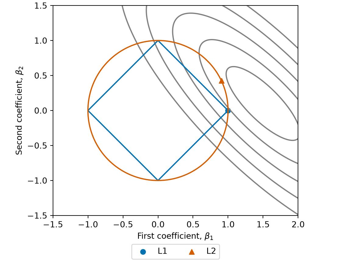
Elliptical contour lines of the squared error, tilted so that they run from upper left to lower right, centred on the least-squares point (1.5, 0.1) outside both regions. A diamond with corners at (+-1, 0) and (0, +-1) and a circle of radius 1 are drawn around the origin. A point marks the best fit inside each region: it sits on the diamond's right corner, (1, 0), and on the circle at about (0.91, 0.43).

The best point in the diamond is \((1, 0)\), the corner on the \(\coef{1}\) axis, where \(\coef{2}\) is exactly zero. The best point in the disc is about \((0.91, 0.43)\), where both coefficients are non-zero. This is the geometric reason the lasso sets coefficients to zero and ridge regression does not (Solution 25). A penalty is the Lagrangian form of such a constraint, so a larger \(\regpar\) corresponds to a smaller ball.

ExrExercise 31 (Count the zero coefficients of ridge and the lasso on baseball salaries)

Exercise 31 (Count the zero coefficients of ridge and the lasso on baseball salaries) Use the Hitters data and the training half of Exercise 4, with the predictors standardized and the salary centered by the training mean. For \(\regpar = 10^2, 10^{2.5}, \dots, 10^5\), fit ridge regression with the closed-form solution of this chapter, and fit the lasso by the coordinate descent of Theorem 2.

Solution 31.

import numpy as np
import pandas as pd

hz_py = pd.read_csv("data/hitters.csv").dropna()
hz_x = pd.get_dummies(hz_py.drop(columns="Salary"), drop_first=True)
hz_names = list(hz_x.columns)
hz_x = hz_x.to_numpy(dtype=float)
hz_y = hz_py["Salary"].to_numpy()

rng = np.random.default_rng(1)
hz_train = rng.permutation(len(hz_y))[: len(hz_y) // 2]

# Standardize with the training half's mean and standard deviation, and center
# the salary, so that no intercept needs to be fit or penalized.
xt = hz_x[hz_train]
xt = (xt - xt.mean(axis=0)) / xt.std(axis=0, ddof=1)
yt = hz_y[hz_train] - hz_y[hz_train].mean()

def ridge_zero_py(lam):
    return np.linalg.solve(xt.T @ xt + lam * np.eye(xt.shape[1]), xt.T @ yt)

def lasso_zero_py(lam, sweeps=200):
    # Coordinate descent: each coefficient in turn is set to the soft-thresholded
    # correlation of its feature with the partial residual, over the feature's
    # sum of squares.
    b = np.zeros(xt.shape[1])
    for _ in range(sweeps):
        for j in range(xt.shape[1]):
            r = yt - xt @ b + xt[:, j] * b[j]
            z = xt[:, j] @ r
            b[j] = np.sign(z) * max(abs(z) - lam / 2, 0.0) / (xt[:, j] @ xt[:, j])
    return b

lams_py = 10.0 ** np.arange(2, 5.5, 0.5)
hz <- na.omit(read.csv("data/hitters.csv"))
hz_x <- model.matrix(Salary ~ ., data = hz)[, -1]

set.seed(1)
hz_train <- sample(nrow(hz), nrow(hz) / 2)

# Standardize with the training half's mean and standard deviation, and center
# the salary, so that no intercept needs to be fit or penalized.
xt <- scale(
  hz_x[hz_train, ],
  center = colMeans(hz_x[hz_train, ]),
  scale = apply(hz_x[hz_train, ], 2, sd)
)
yt <- hz$Salary[hz_train] - mean(hz$Salary[hz_train])

ridge_zero <- function(lambda) {
  drop(solve(crossprod(xt) + lambda * diag(ncol(xt)), crossprod(xt, yt)))
}

lasso_zero <- function(lambda, sweeps = 200) {
  # Coordinate descent: each coefficient in turn is set to the soft-thresholded
  # correlation of its feature with the partial residual, over the feature's
  # sum of squares.
  b <- rep(0, ncol(xt))
  for (s in seq_len(sweeps)) {
    for (j in seq_len(ncol(xt))) {
      r <- yt - xt[, -j, drop = FALSE] %*% b[-j]
      z <- sum(xt[, j] * r)
      b[j] <- sign(z) * max(abs(z) - lambda / 2, 0) / sum(xt[, j]^2)
    }
  }
  b
}

lams <- 10^seq(2, 5, by = 0.5)

The two languages split the players at random in different ways, so their counts differ. The numbers in the later parts of this solution are from the R split.

ExrExercise 32 (Count the zero coefficients of ridge and the lasso on baseball salaries (part 2))

Exercise 32 (Count the zero coefficients of ridge and the lasso on baseball salaries (part 2)) Use the setup of Exercise 31.

For each \(\regpar\), count the coefficients that are exactly zero in each fit.

Solution 32.

pd.DataFrame({
    "lambda": lams_py.round(),
    "ridge_zeros": [int(np.sum(ridge_zero_py(l) == 0)) for l in lams_py],
    "lasso_zeros": [int(np.sum(lasso_zero_py(l) == 0)) for l in lams_py],
})
     lambda  ridge_zeros  lasso_zeros
0     100.0            0            0
1     316.0            0            1
2    1000.0            0            5
3    3162.0            0           12
4   10000.0            0           14
5   31623.0            0           16
6  100000.0            0           19
zero_counts <- data.frame(
  lambda = round(lams),
  ridge_zeros = sapply(lams, function(l) sum(ridge_zero(l) == 0)),
  lasso_zeros = sapply(lams, function(l) sum(lasso_zero(l) == 0))
)
zero_counts

Ridge sets no coefficient to zero at any \(\regpar\) in the grid: the count stays at 0. The lasso’s count climbs from 1 of the 19 coefficients at \(\regpar = 10^2\) to all 19 at \(\regpar = 10^5\).

ExrExercise 33 (Count the zero coefficients of ridge and the lasso on baseball salaries (part 3))

Exercise 33 (Count the zero coefficients of ridge and the lasso on baseball salaries (part 3)) Use the setup of Exercise 31.

Which predictors still have non-zero lasso coefficients at \(\regpar = 10^4\)?

Solution 33.

b_1e4_py = pd.Series(lasso_zero_py(1e4), index=hz_names)
b_1e4_py[b_1e4_py != 0].round()
Hits           65.0
CHmRun         31.0
CRBI          173.0
PutOuts        40.0
Division_W    -60.0
dtype: float64
# The predictors that survive at lambda = 10^4, with their coefficients.
b_1e4 <- setNames(lasso_zero(1e4), colnames(xt))
round(b_1e4[b_1e4 != 0])
     Hits       RBI     Walks     CHits    CHmRun      CRBI DivisionW   PutOuts 
       14         2        84         4        59       125       -42        14 

At \(\regpar = 10^4\), 8 predictors remain: Hits, RBI, Walks, CHits, CHmRun, CRBI, DivisionW, PutOuts.

ExrExercise 34 (Count the zero coefficients of ridge and the lasso on baseball salaries (part 4))

Exercise 34 (Count the zero coefficients of ridge and the lasso on baseball salaries (part 4)) Use the setup of Exercise 31.

How do the counts of exactly zero coefficients compare with your prediction in Exercise 25?

Solution 34. The counts match the prediction of Solution 25: ridge only shrinks, and the lasso selects.

ExrExercise 35 (Choose the lasso penalty by cross-validation on baseball salaries)

Exercise 35 (Choose the lasso penalty by cross-validation on baseball salaries) Use the Hitters data and the standardized training half of Exercise 31. Randomly assign the training players to ten folds. For \(\regpar = 10^{1.5}, 10^2, \dots, 10^{4.5}\), compute the 10-fold cross-validation estimate of the test error of the lasso and of ridge regression, with the lasso computed by the coordinate descent of Theorem 2.

Solution 35.

# The standardized training half xt and centered salary yt are from the previous solution.
ridge_fit <- function(x, y, lambda) {
  drop(solve(crossprod(x) + lambda * diag(ncol(x)), crossprod(x, y)))
}

lasso_fit <- function(x, y, lambda, sweeps = 100) {
  b <- numeric(ncol(x))
  r <- y
  ss <- colSums(x^2)
  for (s in seq_len(sweeps)) {
    for (j in seq_len(ncol(x))) {
      z <- sum(x[, j] * r) + ss[j] * b[j]
      b_new <- sign(z) * max(abs(z) - lambda / 2, 0) / ss[j]
      r <- r - x[, j] * (b_new - b[j])
      b[j] <- b_new
    }
  }
  b
}

set.seed(2)
folds <- sample(rep(1:10, length.out = nrow(xt)))
lams_cv <- 10^seq(1.5, 4.5, by = 0.5)

cv_estimate <- function(fit) {
  sapply(lams_cv, function(lambda) {
    sq <- numeric(nrow(xt))
    for (f in 1:10) {
      held <- folds == f
      b <- fit(xt[!held, ], yt[!held], lambda)
      sq[held] <- (yt[held] - xt[held, ] %*% b)^2
    }
    mean(sq)
  })
}

cv_ridge <- cv_estimate(ridge_fit)
cv_lasso <- cv_estimate(lasso_fit)

data.frame(
  lambda = round(lams_cv),
  ridge_cv_rmse = round(sqrt(cv_ridge)),
  lasso_cv_rmse = round(sqrt(cv_lasso))
)
# The standardized training half xt and centered salary yt are from the previous solution.
def ridge_fit_py(x, y, lam):
    return np.linalg.solve(x.T @ x + lam * np.eye(x.shape[1]), x.T @ y)

def lasso_fit_py(x, y, lam, sweeps=100):
    b = np.zeros(x.shape[1])
    r = y.copy()
    ss = (x ** 2).sum(axis=0)
    for _ in range(sweeps):
        for j in range(x.shape[1]):
            z = x[:, j] @ r + ss[j] * b[j]
            b_new = np.sign(z) * max(abs(z) - lam / 2, 0.0) / ss[j]
            r -= x[:, j] * (b_new - b[j])
            b[j] = b_new
    return b

folds_py = np.random.default_rng(2).permutation(np.arange(len(yt)) % 10)
lams_cv_py = 10.0 ** np.arange(1.5, 4.6, 0.5)

def cv_estimate_py(fit):
    out = []
    for lam in lams_cv_py:
        sq = np.empty(len(yt))
        for f in range(10):
            held = folds_py == f
            b = fit(xt[~held], yt[~held], lam)
            sq[held] = (yt[held] - xt[held] @ b) ** 2
        out.append(sq.mean())
    return np.array(out)

cv_ridge_py = cv_estimate_py(ridge_fit_py)
cv_lasso_py = cv_estimate_py(lasso_fit_py)

pd.DataFrame({
    "lambda": lams_cv_py.round(),
    "ridge_cv_rmse": np.sqrt(cv_ridge_py).round(),
    "lasso_cv_rmse": np.sqrt(cv_lasso_py).round(),
})
    lambda  ridge_cv_rmse  lasso_cv_rmse
0     32.0          371.0          376.0
1    100.0          371.0          375.0
2    316.0          377.0          373.0
3   1000.0          397.0          373.0
4   3162.0          426.0          378.0
5  10000.0          444.0          378.0
6  31623.0          452.0          410.0

The two languages split the players at random in different ways, so their numbers differ. The numbers in the later parts of this solution are from the R split.

ExrExercise 36 (Choose the lasso penalty by cross-validation on baseball salaries (part 2))

Exercise 36 (Choose the lasso penalty by cross-validation on baseball salaries (part 2)) Use the setup of Exercise 35.

For each method, find the \(\regpar\) with the smallest estimate, refit on the whole training half, and compute the root mean squared error on the test half.

Solution 36.

lam_ridge <- lams_cv[which.min(cv_ridge)]
lam_lasso <- lams_cv[which.min(cv_lasso)]
c(ridge = lam_ridge, lasso = lam_lasso)
   ridge    lasso 
 100.000 3162.278 
hc_test <- setdiff(seq_len(nrow(hz)), hz_train)
xte <- scale(
  hz_x[hc_test, ],
  center = colMeans(hz_x[hz_train, ]),
  scale = apply(hz_x[hz_train, ], 2, sd)
)
yte <- hz$Salary[hc_test] - mean(hz$Salary[hz_train])

b_ridge <- ridge_fit(xt, yt, lam_ridge)
b_lasso <- lasso_fit(xt, yt, lam_lasso)
rmse_test <- function(b) sqrt(mean((yte - xte %*% b)^2))
c(ridge = rmse_test(b_ridge), lasso = rmse_test(b_lasso))
   ridge    lasso 
373.9591 378.3654 
lam_ridge_py = lams_cv_py[np.argmin(cv_ridge_py)]
lam_lasso_py = lams_cv_py[np.argmin(cv_lasso_py)]
print("chosen lambda:", lam_ridge_py.round(), lam_lasso_py.round())
chosen lambda: 100.0 316.0
hc_test = np.setdiff1d(np.arange(len(hz_y)), hz_train)
xte = (hz_x[hc_test] - hz_x[hz_train].mean(axis=0)) / hz_x[hz_train].std(axis=0, ddof=1)
yte = hz_y[hc_test] - hz_y[hz_train].mean()

b_ridge_py = ridge_fit_py(xt, yt, lam_ridge_py)
b_lasso_py = lasso_fit_py(xt, yt, lam_lasso_py)
for name, b in [("ridge", b_ridge_py), ("lasso", b_lasso_py)]:
    print(name, round(float(np.sqrt(np.mean((yte - xte @ b) ** 2)))))
ridge 325
lasso 331

Cross-validation chooses \(\regpar =\) 100 for ridge regression and \(\regpar =\) 3162 for the lasso. The test root mean squared error is 374 thousand dollars for ridge regression and 378 for the lasso.

ExrExercise 37 (Choose the lasso penalty by cross-validation on baseball salaries (part 3))

Exercise 37 (Choose the lasso penalty by cross-validation on baseball salaries (part 3)) Use the setup of Exercise 35.

How many lasso coefficients are exactly zero at the chosen \(\regpar\)?

Solution 37.

c(zeros = sum(b_lasso == 0), coefficients = length(b_lasso))
       zeros coefficients 
           8           19 
print(int(np.sum(b_lasso_py == 0)), "of", len(b_lasso_py), "coefficients are zero")
1 of 19 coefficients are zero

At its choice the lasso sets 8 of the 19 coefficients to exactly zero.

ExrExercise 38 (Choose the lasso penalty by cross-validation on baseball salaries (part 4))

Exercise 38 (Choose the lasso penalty by cross-validation on baseball salaries (part 4)) Use the setup of Exercise 35.

Which method predicts the test half better?

Solution 38. Ridge regression has the lower test error, 374 thousand dollars against 378. The test half played no part in choosing either penalty, so these two errors compare the methods fairly.

ReadingRead

The last exercise follows the lab on ridge regression and the lasso in the second edition of the book by James et al. [12, Sec. 6.5.2]. The lab fits the lasso with glmnet; here we use the coordinate descent of this chapter instead. The lab is also available in Python [20] and in R with tidymodels, in ISLR-tidymodels-labs.

6 Norms and sparsity

The count of non-zero coefficients is written \(\norm{\vcoef}_0\) and called the \(\ell_0\) “norm” — in quotes, because it is not one. A norm has to scale with its argument, and doubling every coefficient leaves the count untouched: \(\norm{2\vcoef}_0 =\norm{\vcoef}_0\).

It is also not convex. Convexity is a separate property, and its absence rules out gradient descent. Convexity would require the count at a midpoint to be no more than the average of the counts at the two ends, and it is not: \((1,0)\) and \((0,1)\) each have one non-zero entry, while their midpoint \((\tfrac12,\tfrac12)\) has two.

\[\sumto{i}{d} \mathbf{1}\{\coef{i} \ne 0\} =\norm{\vcoef}_0\]

A sparse vector has a low \(\ell_0\) “norm”.
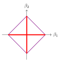
Hand-drawn diagram from Week 4 lecture notes

\[\textcolor{red}{\norm{\vcoef}_0 = 2} \qquad \textcolor{violet}{\sumto{i}{d} |\coef{i}| =\norm{\vcoef}_1 \;\; \text{closest convex function to the } \ell_0 \text{ "norm"}}\]

\[\textcolor{teal}{\sqrt{\sumto{i}{d} |\coef{i}|^2} =\norm{\vcoef}_2}\] \[\sqrt[q]{\sumto{i}{d} |\coef{i}|^q} =\norm{\vcoef}_q \qquad q \geq 1\]

VideosWatch
VideosWatch

Hutchinson teaches parameter norm penalties (L2, L1 and sparsity) (10 min) [23]. The video site requires a login, which enrolled students find in the syllabus.

ReadingRead

GeeksforGeeks compares the lasso, ridge and the elastic net [24].

7 Regularization as prior knowledge

We can read both penalties as prior beliefs. Ridge has a prior that \(\norm{\vcoef}\) is small, and squared error itself assumes the residuals are Gaussian.
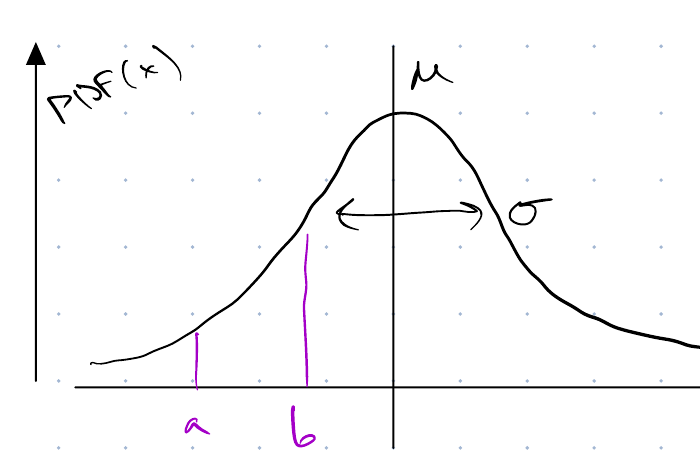
7.1 The normal distribution

Scanned figure from Week 4 lecture notes

\[\Pr[x \in [a,b]] = \int_a^b P(x)\,dx\] \[P(x) = \frac{1}{\sdpar\sqrt{2\pi}} e^{\frac{-1}{2\varpar}(x-\mean)^2}\] \[E[x] = \mean, \qquad \Var{x} = \varpar\]

VideosWatch

Starmer explains the normal distribution [25].

ReadingRead

GeeksforGeeks explains the normal distribution [26].

7.2 Estimating parameters by maximum likelihood

ExmExample 6 (Maximum likelihood for a normal mean)

Example 6 (Maximum likelihood for a normal mean) Take a sample of \(n = 5\) observations, \(x: (2,5,4,12,7)\), drawn independently from that normal distribution, and ask which \(\mean\) makes them most likely.

\[\Pr(\text{data} \mid \mean) = P(x_1)\cdot P(x_2) \cdots P(x_n)\]

\[ \begin{aligned} &= \prodin \frac{1}{\sdpar\sqrt{2\pi}} e^{-\frac{1}{2\varpar}(x_i-\mean)^2} \\ &= (\sdpar\sqrt{2\pi})^{-n} e^{-\frac{1}{2\varpar}\sumin (x_i-\mean)^2} \end{aligned} \]

\[\hmean = \argmax_\mean \Pr(\text{data}\mid \mean)\] \[ \begin{aligned} \hmean &= \argmax_\mean \log\Pr(\text{data}\mid \mean) \\ &= \argmin_\mean -\log\Pr(\text{data}\mid \mean) \qquad \textcolor{green}{\text{Negative log-likelihood}} \end{aligned} \]

\[L(\mean) = -\log(\sdpar\sqrt{2\pi})^{-n} - \paren{-\frac{1}{2\varpar}\sumin (x_i-\mean)^2}\] \[= \text{const in } \mean + \frac{1}{2\varpar}\sumin (x_i-\mean)^2 \qquad \textcolor{gray}{\mean \text{ acts like } \coef{0}}\]

\[\hmean = \avgin x_i\]

So the maximum-likelihood estimate of a normal mean is just the sample mean. On the sample of five,

\[ \begin{aligned} \hmean &= \tfrac{1}{5}(2+5+4+12+7) \\ &= \tfrac{30}{5} \\ &= 6. \end{aligned} \]

ReadingRead

GeeksforGeeks explains maximum likelihood estimation [29].

7.3 Priors and Bayes’ rule

  1. A model of the probability of the data gives \(\Pr(\text{data} \mid \text{parameters})\).

  2. Priors on the parameters give \(\Pr(\text{parameters})\).

  3. Bayes’ rule gives \(\Pr(\text{parameters} \mid \text{data})\).

\[\fbox{$P(A \mid B)$} = \frac{\fbox{$P(B\mid A)$}\cdot \fbox{$P(A)$}}{P(B)} \qquad \textcolor{teal}{P(B\mid A)\,P(A) = P(A \cap B)}\]
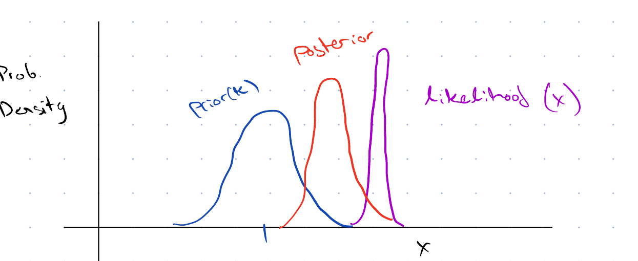
Scanned figure from Week 4 lecture notes

VideosWatch

Starmer explains Bayes’ theorem [30].

ReadingRead

GeeksforGeeks explains Bayes’ theorem [31].

7.4 Ridge regression as a Gaussian prior

\[\min_{\vcoef} \;\underbrace{\norm{X\vcoef - \vy}^2}_{\textcolor{violet}{\text{likelihood}}} + \underbrace{\regpar\norm{\vcoef}^2}_{\textcolor{blue}{\text{prior}}} \qquad \underbrace{\phantom{\norm{X\vcoef - \vy}^2 + \regpar\norm{\vcoef}^2}}_{\textcolor{red}{\propto\; -\log \Pr(\vcoef \mid X, \vy)}} \qquad \textcolor{blue}{\vcoef \sim N(0,\regpar^{-1} I)}\]

\[-\log \Pr(\vcoef \mid x,y) = -\log\paren{\frac{P(x,y\mid \vcoef)\cdot P(\vcoef)}{P(x,y)}}\]

Writing out the likelihood,

\[-\log P(\text{data} \mid \vcoef) = \frac{1}{2\varpar}\sumin \paren{\dprod{\vx_i}{\vcoef} - y_i}^2 + \text{const}\]

and the Gaussian prior,

\[ \begin{aligned} P(\vcoef) &= \prod_{i=1}^d \frac{\sqrt{\regpar}}{\sqrt{2\pi}} e^{-\regpar/2\,\coef{i}^2} \\ &= \paren{\frac{\regpar}{2\pi}}^{d/2} e^{-\frac{\regpar}{2}\paren{\coef{1}^2+\coef{2}^2+\dots+\coef{d}^2}} \end{aligned} \]

\[P(\vcoef \mid \text{data}) = \frac{P(\text{data}\mid \vcoef)\cdot P(\vcoef)}{P(\text{data})}\] \[-\log P(\vcoef\mid\text{data}) = -\log P(\text{data}\mid \vcoef) - \log P(\vcoef) + \textcolor{red}{\log P(\text{data})} \quad \textcolor{red}{\leftarrow \text{ignore}}\]

\[-\log P(\vcoef\mid\text{data}) = \frac{1}{2\varpar}\sumin \paren{\dprod{\vx_i}{\vcoef} - y_i}^2 + \frac{\regpar}{2}\sumto{i}{d} \coef{i}^2 + \text{const}\]

Multiplying through by \(2\varpar\) does not move the minimizer, so writing \(\regpar' = \varpar\regpar\) recovers the familiar form:

\(\displaystyle \min_{\vcoef}\; \sumin \paren{\dprod{\vx_i}{\vcoef} - y_i}^2 + \regpar'\sumto{i}{d} \coef{i}^2\) Ridge

\(\uparrow\) Gaussian prior on \(\coef{i}\)’s (\(\regpar\) large)
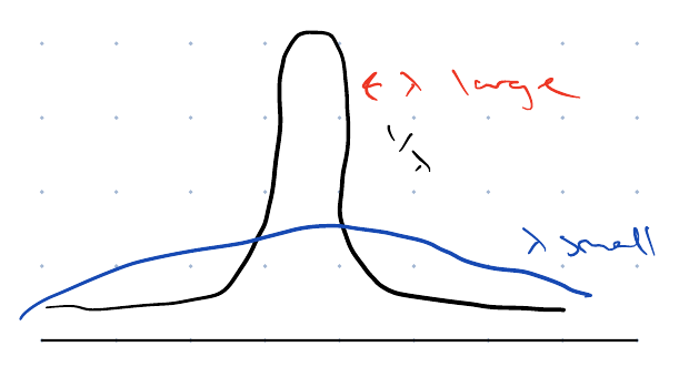
Scanned figure from Week 4 lecture notes

So ridge regression is maximum a posteriori estimation under a Gaussian prior on the coefficients, and the lasso is the same thing under a Laplace prior. Regularizing is not an unprincipled fix: it states explicitly what we believe about the coefficients before we see the data.

ReadingRead

GeeksforGeeks explains maximum a posteriori estimation [32].

8 Regularizing by dimension reduction

Ridge regression and the lasso keep every feature and penalize its coefficient. A third route replaces the \(\ninputvars\) features by a few combinations of them, and fits least squares on the combinations. That constrains the coefficient vector to a small space of directions, and so it lowers the variance, as the penalty does. The two methods below differ in how they pick the combinations: principal components regression uses only the features, and partial least squares uses the response too [12, Sec. 6.3].

ExrExercise 39 (Predict baseball salaries from a few combinations of the predictors)

Exercise 39 (Predict baseball salaries from a few combinations of the predictors) Ridge regression and the lasso keep all 19 predictors of the Hitters data and penalize their coefficients. Here we instead replace the predictors by \(M\) linear combinations of them, and fit least squares on those combinations alone. We build the combinations in two ways.

  • Greatest variance of the predictors. Take the first \(M\) directions, in order, along which the standardized training predictors vary most. These are the first \(M\) right singular vectors of the standardized training predictor matrix (see principal component analysis). Each combination weights the predictors by the entries of one singular vector.

  • Relation to the salary. Weight each standardized predictor by its simple regression coefficient on the centered salary, and add the weighted predictors to make the first combination. Subtract from every predictor the part of it that the first combination explains, by regressing each predictor on the combination and keeping the residuals. Build the second combination from the residuals in the same way, and repeat.

Use the training half and the standardized predictors of Exercise 4, and the ten folds of Exercise 8. For each way and each \(M = 0, 1, \dots, 19\), compute the 10-fold cross-validation estimate. Take \(M = 0\) to predict the training mean salary for every player.

Solution 39. The first way is principal components regression and the second is partial least squares, both defined in this section. Each is a linear combination of the standardized predictors, so each fit has one coefficient per predictor.

For the second way, the residual of a predictor after regressing on a combination \(\vz\) is \(x_j - \vz\,\dprod{\vz}{x_j}/\dprod{\vz}{\vz}\), so after \(m - 1\) combinations the residual predictors are \(X\prod_{k<m}\paren{I - \vphi_k\tp{\vp_k}}\), where \(\vphi_k\) holds the weights of combination \(k\) and \(\vp_k\) the regression coefficients of the predictors on it. That lets the code express every combination in the original standardized predictors.

xs_tr <- Xs[train, ]
y_tr <- y[train]
d <- ncol(xs_tr)

pls_dirs <- function(x, y, m) {
  # Columns are the weights of each combination on the original predictors.
  proj <- diag(ncol(x))
  xk <- x
  out <- matrix(0, ncol(x), m)
  for (k in seq_len(m)) {
    phi <- drop(crossprod(xk, y)) / colSums(xk^2)
    z <- drop(xk %*% phi)
    p <- drop(crossprod(xk, z)) / sum(z^2)
    out[, k] <- proj %*% phi
    proj <- proj %*% (diag(ncol(x)) - outer(phi, p))
    xk <- xk - outer(z, p)
  }
  out
}

fit_predict <- function(x, y, m, method, x_new) {
  x_bar <- colMeans(x)
  x_c <- sweep(x, 2, x_bar)
  y_c <- y - mean(y)
  if (m == 0) {
    return(rep(mean(y), nrow(x_new)))
  }
  w <- if (method == "pcr") svd(x_c, nu = 0, nv = m)$v else pls_dirs(x_c, y_c, m)
  z <- x_c %*% w
  beta <- drop(w %*% solve(crossprod(z), crossprod(z, y_c)))
  mean(y) + drop(sweep(x_new, 2, x_bar) %*% beta)
}

methods <- c("pcr", "pls")
cv_sq_dr <- lapply(setNames(methods, methods), function(meth) {
  sq <- matrix(0, length(y_tr), d + 1)
  for (f in seq_len(k_cv)) {
    held <- fold == f
    for (m in 0:d) {
      pred <- fit_predict(xs_tr[!held, ], y_tr[!held], m, meth, xs_tr[held, , drop = FALSE])
      sq[held, m + 1] <- (y_tr[held] - pred)^2
    }
  }
  sq
})

library(ggplot2)
cv_curves <- do.call(rbind, lapply(methods, function(meth) {
  data.frame(method = meth, m = 0:d, cv_rmse = sqrt(colMeans(cv_sq_dr[[meth]])))
}))
ggplot(cv_curves, aes(m, cv_rmse, colour = method)) +
  geom_line() +
  geom_point() +
  labs(x = "number of combinations (M)", y = "cross-validation RMSE (thousand dollars)", colour = NULL) +
  theme(legend.position = "bottom")
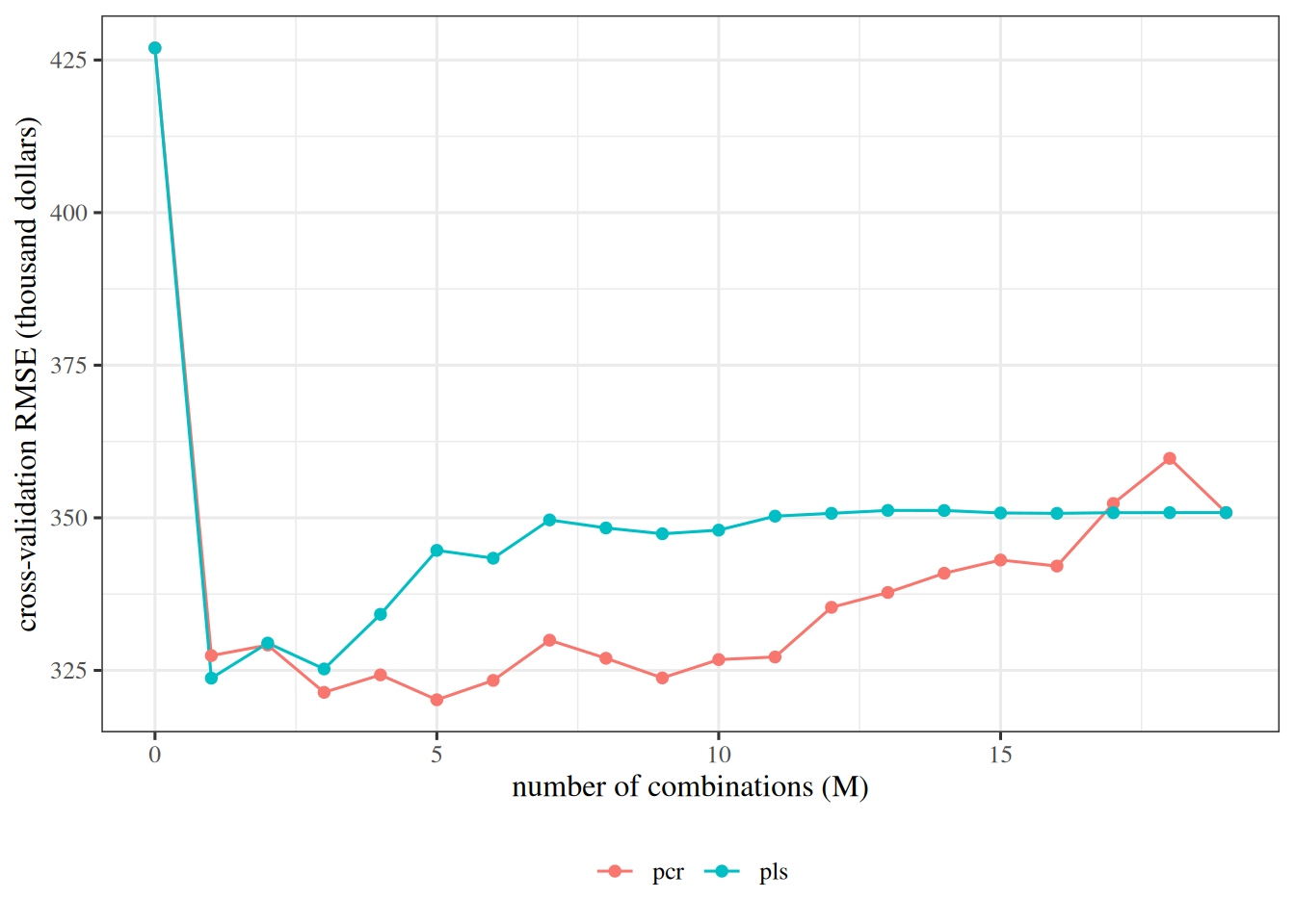
Cross-validation root mean squared error against the number of combinations, from 0 to 19, for principal components regression and for partial least squares on the Hitters training half. Both start high at zero combinations, which predicts the mean salary, and fall sharply at one combination. Partial least squares has its lowest value at one or a few combinations and then rises. Principal components regression stays low for more combinations, and then rises. At 19 combinations both curves reach the same value, that of least squares on all the predictors.

xs_tr_py = X_py[train_py, 1:]
y_tr_py = y_py[train_py]
d_py = xs_tr_py.shape[1]


def pls_dirs_py(x, y, m):
    # Columns are the weights of each combination on the original predictors.
    proj = np.eye(x.shape[1])
    xk = x
    out = np.zeros((x.shape[1], m))
    for k in range(m):
        phi = (xk.T @ y) / (xk ** 2).sum(axis=0)
        z = xk @ phi
        p = (xk.T @ z) / (z @ z)
        out[:, k] = proj @ phi
        proj = proj @ (np.eye(x.shape[1]) - np.outer(phi, p))
        xk = xk - np.outer(z, p)
    return out


def fit_predict_py(x, y, m, method, x_new):
    x_bar = x.mean(axis=0)
    x_c, y_c = x - x_bar, y - y.mean()
    if m == 0:
        return np.full(len(x_new), y.mean())
    w = (np.linalg.svd(x_c, full_matrices=False)[2][:m].T
         if method == "pcr" else pls_dirs_py(x_c, y_c, m))
    z = x_c @ w
    beta = w @ np.linalg.solve(z.T @ z, z.T @ y_c)
    return y.mean() + (x_new - x_bar) @ beta


methods_py = ["pcr", "pls"]
cv_sq_dr_py = {meth: np.empty((len(y_tr_py), d_py + 1)) for meth in methods_py}
for meth in methods_py:
    for f in range(k_cv):
        held = fold_py == f
        for m in range(d_py + 1):
            pred = fit_predict_py(xs_tr_py[~held], y_tr_py[~held], m, meth, xs_tr_py[held])
            cv_sq_dr_py[meth][held, m] = (y_tr_py[held] - pred) ** 2

fig, ax = plt.subplots(figsize=(6, 4), layout="constrained")
for meth in methods_py:
    ax.plot(range(d_py + 1), np.sqrt(cv_sq_dr_py[meth].mean(axis=0)), marker="o", label=meth);
ax.set_xlabel("number of combinations (M)");
ax.set_ylabel("cross-validation RMSE (thousand dollars)");
ax.legend();
plt.show()
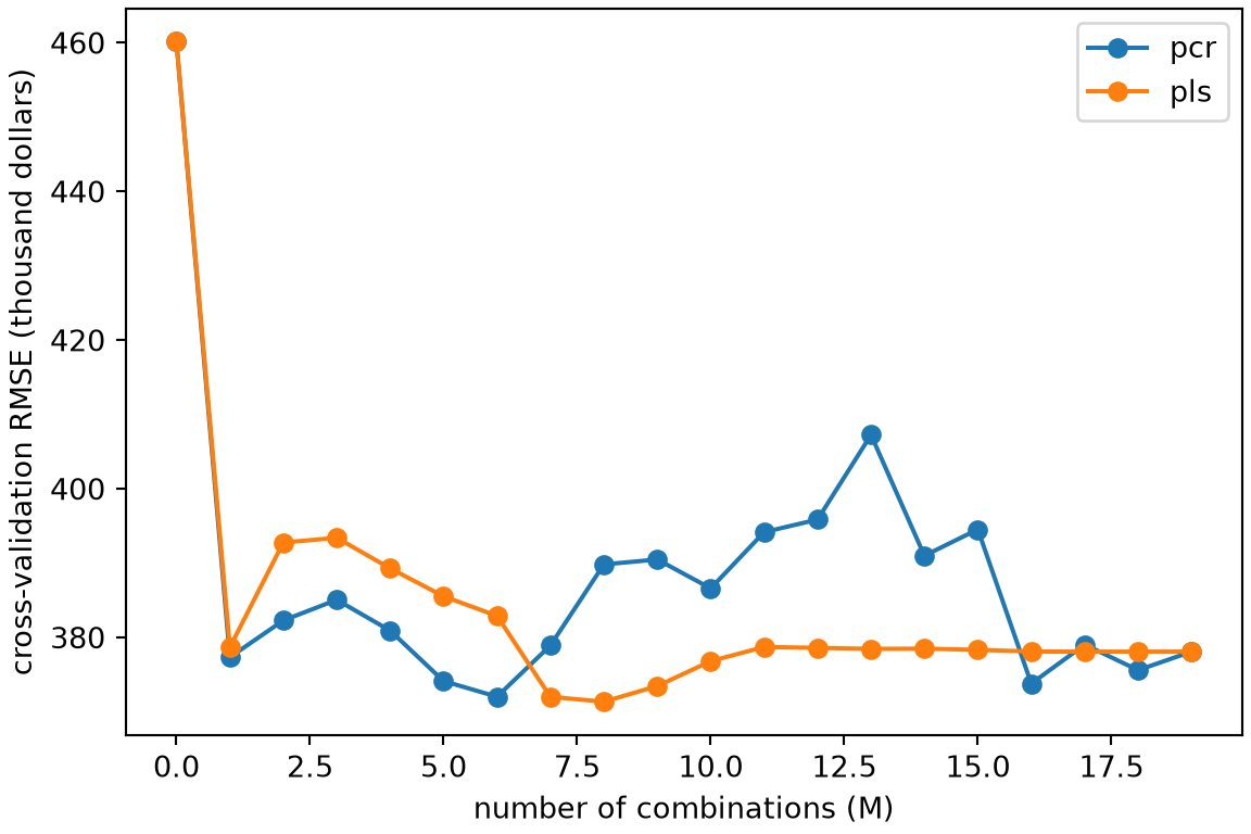
Cross-validation root mean squared error against the number of combinations, from 0 to 19, for principal components regression and for partial least squares on the Hitters training half. Both start high at zero combinations, which predicts the mean salary, and fall sharply at one combination. Partial least squares has its lowest value at one or a few combinations and then rises. Principal components regression stays low for more combinations, and then rises. At 19 combinations both curves reach the same value, that of least squares on all the predictors.

The numbers in the later parts of this solution are from the R split and its folds. With \(M = 19\) both ways give the least squares fit on all the predictors.

ExrExercise 40 (Predict baseball salaries from a few combinations of the predictors (part 2))

Exercise 40 (Predict baseball salaries from a few combinations of the predictors (part 2)) Use the setup of Exercise 39.

For each way, which \(M\) has the smallest estimate?

Solution 40.

dr_cv <- sapply(cv_sq_dr, function(sq) sqrt(colMeans(sq)))
dr_m <- apply(dr_cv, 2, which.min) - 1
rbind(M = dr_m, cv_rmse = apply(dr_cv, 2, min))
            pcr      pls
M         5.000   1.0000
cv_rmse 320.188 323.7307
for meth in methods_py:
    cv_m = cv_sq_dr_py[meth].mean(axis=0)
    m_best = int(np.argmin(cv_m))
    print(meth, "- M", m_best, "- cv sRMSE", round(float(np.sqrt(cv_m[m_best]))))
pcr - M 6 - cv sRMSE 372
pls - M 8 - cv sRMSE 371

Principal components regression chooses \(M =\) 5 combinations, and partial least squares chooses \(M =\) 1.

ExrExercise 41 (Predict baseball salaries from a few combinations of the predictors (part 3))

Exercise 41 (Predict baseball salaries from a few combinations of the predictors (part 3)) Use the setup of Exercise 39.

Compute the test errors of the two choices.

Solution 41.

dr_test <- sapply(methods, function(meth) {
  pred <- fit_predict(xs_tr, y_tr, dr_m[[meth]], meth, Xs[-train, ])
  sqrt(mean((y[-train] - pred)^2))
})
dr_summary <- data.frame(
  method = methods, m = unname(dr_m),
  cv_rmse = unname(apply(dr_cv, 2, min)), test_rmse = unname(dr_test)
)
dr_summary
for meth in methods_py:
    m_best = int(np.argmin(cv_sq_dr_py[meth].mean(axis=0)))
    pred = fit_predict_py(xs_tr_py, y_tr_py, m_best, meth, X_py[test_py, 1:])
    test_rmse_dr = np.sqrt(np.mean((y_py[test_py] - pred) ** 2))
    print(meth, "- test sRMSE", round(float(test_rmse_dr)))
pcr - test sRMSE 323
pls - test sRMSE 334

The test root mean squared error (RMSE) is 378 thousand dollars for principal components regression and 390 for partial least squares.

ExrExercise 42 (Predict baseball salaries from a few combinations of the predictors (part 4))

Exercise 42 (Predict baseball salaries from a few combinations of the predictors (part 4)) Use the setup of Exercise 39.

How do the test errors of the two choices compare with that of ridge regression at the penalty chosen in Exercise 9?

Solution 42. Ridge regression at the penalty chosen in Solution 9 has a test RMSE of 376, against 378 for principal components regression and 390 for partial least squares.

ReadingRead

This exercise follows the lab on principal components regression and partial least squares in the second edition of the book by James et al. [12, Sec. 6.5.3]. The lab uses the pls package; here we compute the directions ourselves.

DefDefinition 4 (Derived feature)

Definition 4 (Derived feature) Let \(X\) be an \(n \times \ninputvars\) matrix of features whose columns have mean zero, and let \(\vphi \in \reals^{\ninputvars}\). The derived feature with loadings \(\vphi\) is the vector \(\vz = X\vphi \in \reals^n\), whose \(i\)th entry is

\[ z_i = \sum_{j=1}^{\ninputvars} \phi_j x_{ij}. \]

It is one new feature, a weighted sum of the original features, for each of the \(n\) observations.

ExmExample 7 (The average of two standardized batting statistics)

Example 7 (The average of two standardized batting statistics) Take two batting statistics of the 1986 Hitters: the number of times at bat (AtBat) and the number of hits (Hits). Standardize each, so that its mean is zero and its standard deviation is one, and take the loadings \(\vphi = \tp{[1/\sqrt{2},\, 1/\sqrt{2}]}\).

Show code
dr_x <- scale(hit[, c("AtBat", "Hits")])
dr_y <- hit$Salary
dr_phi <- c(1, 1) / sqrt(2)
dr_z <- drop(dr_x %*% dr_phi)
head(cbind(dr_x, derived = dr_z), 3)
       AtBat       Hits    derived
2 -0.6017532 -0.5945419 -0.8459084
3  0.5115664  0.4913228  0.7091498
4  0.6269715  0.7350884  0.9631217

The first player has \(z_1 = 0.707 \times \paren{-0.602} + 0.707 \times \paren{-0.595} = -0.846\). The derived feature is large for players who are high on both statistics.

DefDefinition 5 (Dimension reduction regression)

Definition 5 (Dimension reduction regression) Let \(X\) be an \(n \times \ninputvars\) matrix of features whose columns have mean zero, let \(\vy \in \reals^n\), and let \(M \le \ninputvars\). Let \(\vz_1, \dots, \vz_M\) be derived features with loadings \(\vphi_1, \dots, \vphi_M\). Dimension reduction regression with these loadings predicts \(y_i\) by

\[ \th_0 + \sum_{m=1}^{M} \th_m z_{im}, \]

where \(\th_0, \th_1, \dots, \th_M\) are the least squares estimates of the regression of \(\vy\) on \(\vz_1, \dots, \vz_M\). It estimates \(M + 1\) coefficients instead of the \(\ninputvars + 1\) of least squares on the original features.

ExmExample 8 (One derived feature predicts salary)

Example 8 (One derived feature predicts salary) Regress the salary of the 1986 Hitters on the single derived feature of Example 7.

Show code
dr_fit <- lm(dr_y ~ dr_z)
coef(dr_fit)
(Intercept)        dr_z 
   535.9259    135.3688 

With \(M = 1\) we estimate \(2\) coefficients, instead of the \(3\) for the two statistics separately. Each additional unit of the derived feature goes with a salary difference of \(135\) thousand dollars.

PrpProposition 1 (The coefficients of a dimension reduction regression)

Proposition 1 (The coefficients of a dimension reduction regression) In the setting of Definition 5, let \(\Phi = [\vphi_1, \dots, \vphi_M]\) be the \(\ninputvars \times M\) matrix of loadings, and let \(\vth = \tp{[\th_1, \dots, \th_M]}\). The prediction for an observation with centered features \(\vx \in \reals^{\ninputvars}\) is

\[ \th_0 + \tp{\vx}\vcoef, \qquad \vcoef = \Phi\vth. \]

So the model is linear in the original features, and its coefficient vector \(\vcoef\) is a combination of the loadings.

Proof. The derived features of the observation are \(z_m = \tp{\vphi_m}\vx\), so \(\sum_m \th_m z_m = \sum_m \th_m \tp{\vphi_m}\vx = \tp{\vx}\Phi\vth\).

ExmExample 9 (The two coefficients of the average)

Example 9 (The two coefficients of the average) For the fit of Example 8, \(\Phi = \vphi\) is a single column, so \(\vcoef = \th_1\vphi\). Least squares on the two statistics themselves is free to choose any two coefficients.

Show code
rbind(
  dimension_reduction = coef(dr_fit)[["dr_z"]] * dr_phi,
  least_squares = coef(lm(dr_y ~ dr_x))[-1]
)
                     dr_xAtBat  dr_xHits
dimension_reduction   95.72017  95.72017
least_squares       -179.12499 370.56533

The dimension reduction fit gives both statistics the same coefficient, \(95.7\), because their loadings are equal. Least squares gives them coefficients of -179.1 and 370.6. The constraint \(\vcoef = \Phi\vth\) has a cost in bias, and it removes the freedom that makes least squares vary from sample to sample when the features are correlated.

DefDefinition 6 (Principal components regression (PCR))

Definition 6 (Principal components regression (PCR)) Let \(X\) be an \(n \times \ninputvars\) matrix of features whose columns have mean zero, with the singular value decomposition \(X = US\tp{V}\), and let \(M \le \ninputvars\). Principal components regression (PCR) with \(M\) components is the dimension reduction regression whose loadings are the first \(M\) columns \(\vv_1, \dots, \vv_M\) of \(V\). These are the first \(M\) principal component loadings of the features, so the derived features \(\vz_m = X\vv_m = \singval_m\vu_m\) are the first \(M\) principal component scores.

ExmExample 10 (Principal components of two batting statistics)

Example 10 (Principal components of two batting statistics) Take the standardized AtBat and Hits of Example 7. We compute the singular value decomposition of the standardized matrix and regress salary on the first score.

Show code
dr_svd <- svd(dr_x)
dr_v <- dr_svd$v
# A singular vector's sign is arbitrary; make the first entry of each positive.
dr_v <- sweep(dr_v, 2, sign(dr_v[1, ]), "*")
dr_scores <- dr_x %*% dr_v
dr_share <- dr_svd$d^2 / sum(dr_svd$d^2)
dr_pcr <- lm(dr_y ~ dr_scores[, 1])
list(loadings = dr_v, share_of_variance = dr_share, pcr_coefficients = coef(dr_pcr))
$loadings
          [,1]       [,2]
[1,] 0.7071068  0.7071068
[2,] 0.7071068 -0.7071068

$share_of_variance
[1] 0.98198456 0.01801544

$pcr_coefficients
   (Intercept) dr_scores[, 1] 
      535.9259       135.3688 

The first loading vector is \((0.707, 0.707)\), nearly the average of the two statistics, because AtBat and Hits are strongly correlated (their sample correlation is 0.96). It accounts for 98.2% of the variance of the two statistics together. PCR with \(M = 1\) regresses salary on that one score, and with \(M = 2\) it would use both scores and give the least squares fit on the two statistics.

DefDefinition 7 (Partial least squares regression (PLS))

Definition 7 (Partial least squares regression (PLS)) Let \(X\) be an \(n \times \ninputvars\) matrix of features whose columns have mean zero and the same standard deviation, let \(\vy \in \reals^n\) have mean zero, and let \(M \le \ninputvars\). Set \(X^{(1)} = X\). For \(m = 1, \dots, M\), with \(X^{(m)}_{\cdot j}\) the \(j\)th column of \(X^{(m)}\):

  1. Compute the loadings \(\phi_{jm} = \dprod{X^{(m)}_{\cdot j}}{\vy} \big/ \dprod{X^{(m)}_{\cdot j}}{X^{(m)}_{\cdot j}}\), the coefficient of the simple regression of \(\vy\) on column \(j\).

  2. Compute the derived feature \(\vz_m = X^{(m)}\vphi_m\).

  3. Replace each column by its residual from the simple regression on \(\vz_m\): \(X^{(m+1)}_{\cdot j} = X^{(m)}_{\cdot j} - \vz_m \dprod{\vz_m}{X^{(m)}_{\cdot j}} \big/ \dprod{\vz_m}{\vz_m}\).

Partial least squares regression (PLS) with \(M\) directions is the least squares regression of \(\vy\) on \(\vz_1, \dots, \vz_M\). Assume every denominator above is non-zero.

ExmExample 11 (The first partial least squares direction of two batting statistics)

Example 11 (The first partial least squares direction of two batting statistics) Use the standardized AtBat and Hits of Example 7, and the salary centered at its mean. The loadings \(\phi_{j1}\) of the first direction are the simple regression coefficients of the salary on each statistic.

Show code
dr_yc <- dr_y - mean(dr_y)
dr_pls_phi <- drop(crossprod(dr_x, dr_yc)) / colSums(dr_x^2)
dr_pls_dir <- dr_pls_phi / sqrt(sum(dr_pls_phi^2))
dr_angle <- acos(abs(sum(dr_pls_dir * dr_v[, 1]))) * 180 / pi
rbind(pls_loadings = dr_pls_phi, pls_unit_direction = dr_pls_dir, first_pc = dr_v[, 1])
                         AtBat        Hits
pls_loadings       178.0885478 197.8943690
pls_unit_direction   0.6689307   0.7433247
first_pc             0.7071068   0.7071068

The salary has a simple regression coefficient of 178.1 on AtBat and 197.9 on Hits, so the first partial least squares direction puts weight \(0.743\) on Hits and \(0.669\) on AtBat, after scaling it to unit length. The first principal component weighs them almost equally. The two directions make an angle of \(3^\circ\): the principal component direction uses only the predictors, and the partial least squares direction also uses the salary.

Show code
library(ggplot2)
dirs <- data.frame(
  direction = c("first principal component", "second principal component",
                "first partial least squares"),
  dx = c(dr_v[1, 1], dr_v[1, 2], dr_pls_dir[1]),
  dy = c(dr_v[2, 1], dr_v[2, 2], dr_pls_dir[2])
)
ggplot() +
  geom_point(aes(AtBat, Hits), data = as.data.frame(dr_x), alpha = 0.4) +
  geom_abline(
    aes(slope = dy / dx, intercept = 0, colour = direction), data = dirs
  ) +
  coord_equal() +
  labs(x = "AtBat (standardized)", y = "Hits (standardized)", colour = NULL) +
  theme(legend.position = "bottom", legend.direction = "vertical")
Show code
import matplotlib.pyplot as plt
import numpy as np
import pandas as pd

hit2 = pd.read_csv("data/hitters.csv").dropna()
x2 = hit2[["AtBat", "Hits"]].to_numpy()
x2 = (x2 - x2.mean(axis=0)) / x2.std(axis=0, ddof=1)
y2 = hit2["Salary"].to_numpy()

v2 = np.linalg.svd(x2, full_matrices=False)[2].T
phi2 = x2.T @ (y2 - y2.mean()) / (x2 ** 2).sum(axis=0)
pls2 = phi2 / np.linalg.norm(phi2)

fig, ax = plt.subplots(figsize=(5, 4), layout="constrained")
ax.scatter(x2[:, 0], x2[:, 1], alpha=0.4);
t = np.array([-3.0, 3.0])
for name, d in [("first principal component", v2[:, 0]),
                ("second principal component", v2[:, 1]),
                ("first partial least squares", pls2)]:
    ax.plot(t * d[0], t * d[1], label=name);
ax.set_xlim(-3, 3);
ax.set_ylim(-3, 3);
ax.set_aspect("equal");
ax.set_xlabel("AtBat (standardized)");
ax.set_ylabel("Hits (standardized)");
fig.legend(loc="outside lower center");
plt.show()
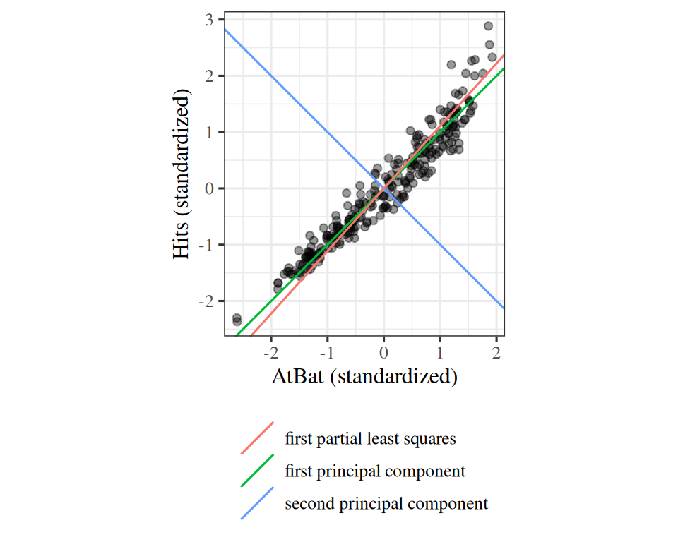
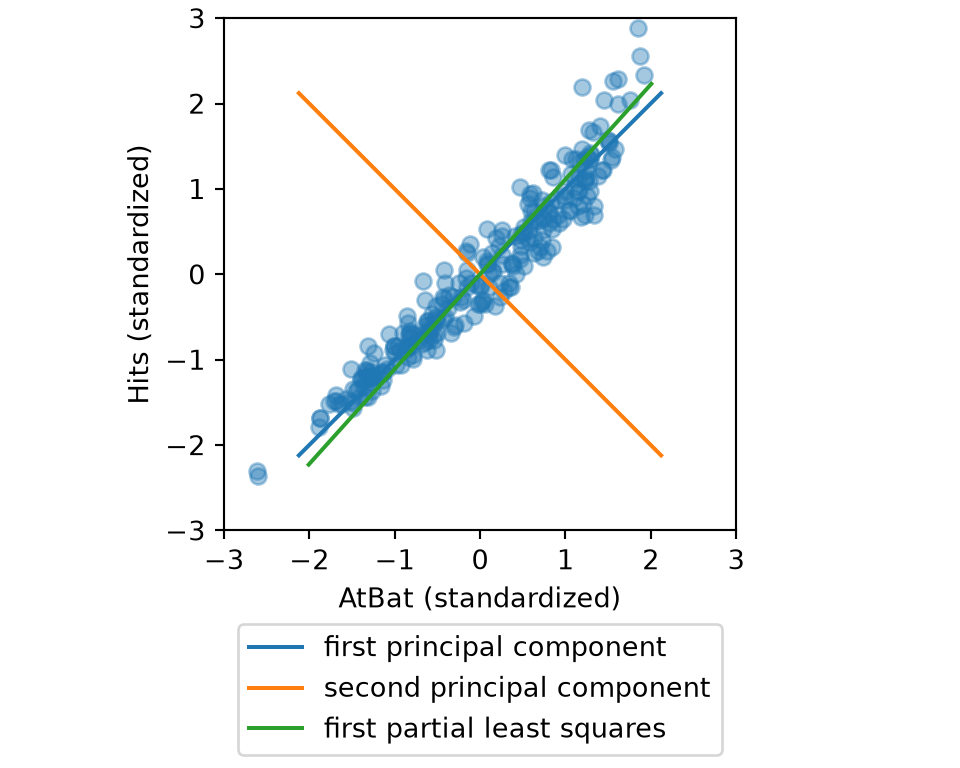
Figure 3: The first principal component runs along the cloud of points. The first partial least squares direction is tilted toward the statistic that is more strongly related to the salary.
(a)
Scatter plot of the standardized number of hits against the standardized number of times at bat for 263 baseball players, with values from about -2.5 to 3. The points lie close to a line rising at about 45 degrees. Three lines through the origin are drawn: the first principal component direction, nearly at 45 degrees along the points, the second principal component direction perpendicular to it, and the first partial least squares direction, rotated slightly from the first principal component toward the hits axis.
(b)
Scatter plot of the standardized number of hits against the standardized number of times at bat for 263 baseball players, with values from about -2.5 to 3. The points lie close to a line rising at about 45 degrees. Three lines through the origin are drawn: the first principal component direction, nearly at 45 degrees along the points, the second principal component direction perpendicular to it, and the first partial least squares direction, rotated slightly from the first principal component toward the hits axis.
RemarkRemark 1 (Principal components regression does not select features)

Remark 1 (Principal components regression does not select features). Every derived feature of PCR is a combination of all \(\ninputvars\) features, so PCR does not set any feature’s coefficient to zero, as the lasso does. In this sense it is closer to ridge regression, which also keeps every feature; in fact ridge regression can be viewed as a continuous version of PCR [12, Sec. 6.3.1]. PCR uses the response only in the final least squares step, so it assumes that the directions in which the features vary most are the ones that predict the response. Partial least squares drops that assumption by using the response to pick the directions, which can lower the bias but can also raise the variance, and in practice it often predicts no better than ridge regression or PCR [12, Sec. 6.3.2]. Standardize the features before using either method, so that a feature measured on a large scale does not dominate the directions.

9 High-dimensional data

The methods above matter most when the data have as many features as observations, or more. Least squares then has no unique solution, as in Underdetermined problems, and it fits the noise in the training data exactly [12, Sec. 6.4].

DefDefinition 8 (High-dimensional data set)

Definition 8 (High-dimensional data set) A data set with \(n\) observations and \(\ninputvars\) features is high-dimensional when \(\ninputvars \ge n\). Some authors also call a data set high-dimensional when \(\ninputvars\) is merely close to \(n\) or larger than a few times \(n\), because the troubles below begin before \(\ninputvars\) reaches \(n\) [12, Sec. 6.4].

ExmExample 12 (Baseball salaries with every pairwise product)

Example 12 (Baseball salaries with every pairwise product) The Hitters data have 19 features. Add the product of every pair of features, which lets the fitted model describe how two statistics work together.

Show code
hd_x <- model.matrix(Salary ~ .^2, hz)[, -1]
c(observations = length(hz_train), features = ncol(hd_x))
observations     features 
         131          190 

On the 131 players of the training half, 190 features is more than 131 observations, so the training half is a high-dimensional data set. The same features on all 263 players would not be: whether a data set is high-dimensional depends on how many observations are available.

ExrExercise 43 (Fit least squares as the features outnumber the observations)

Exercise 43 (Fit least squares as the features outnumber the observations) Simulate \(n = 30\) training observations of \(90\) features, each drawn independently from the standard normal distribution. Let the response equal twice the sum of the first five features, plus noise with standard deviation \(3\). Simulate \(1000\) new observations in the same way.

Solution 43.

set.seed(3)
n_hd <- 30
d_grid <- c(5, 10, 20, 28, 30, 32, 40, 60, 90)
d_max <- max(d_grid)
n_new <- 1000
true_coef <- c(rep(2, 5), rep(0, d_max - 5))

x_hd <- matrix(rnorm(n_hd * d_max), n_hd, d_max)
y_hd <- drop(x_hd %*% true_coef) + rnorm(n_hd, sd = 3)
x_new <- matrix(rnorm(n_new * d_max), n_new, d_max)
y_new <- drop(x_new %*% true_coef) + rnorm(n_new, sd = 3)
rng = np.random.default_rng(3)
n_hd = 30
d_grid = [5, 10, 20, 28, 30, 32, 40, 60, 90]
d_max = max(d_grid)
n_new = 1000
true_coef = np.r_[np.full(5, 2.0), np.zeros(d_max - 5)]

x_hd_py = rng.standard_normal((n_hd, d_max))
y_hd_py = x_hd_py @ true_coef + 3 * rng.standard_normal(n_hd)
x_new_py = rng.standard_normal((n_new, d_max))
y_new_py = x_new_py @ true_coef + 3 * rng.standard_normal(n_new)

The two languages draw different random numbers, so their values differ.

ExrExercise 44 (Fit least squares as the features outnumber the observations (part 2))

Exercise 44 (Fit least squares as the features outnumber the observations (part 2)) Use the setup of Exercise 43.

For each number of features \(\ninputvars = 5, 10, 20, 28, 30, 32, 40, 60, 90\), use the first \(\ninputvars\) features to fit least squares to the training observations. When \(\ninputvars \ge n\) many coefficient vectors fit the training observations equally well, so take the one with the smallest norm, which the pseudoinverse gives. Compute the training \(R^2\) and the mean squared error on the new observations.

Solution 44.

pinv <- function(x, tol = 1e-10) {
  s <- svd(x)
  keep <- s$d > tol * s$d[1]
  s$v[, keep, drop = FALSE] %*% (t(s$u[, keep, drop = FALSE]) / s$d[keep])
}

hd_fit <- t(sapply(d_grid, function(d) {
  x <- x_hd[, 1:d, drop = FALSE]
  b <- drop(pinv(x) %*% y_hd)
  c(
    D = d,
    train_r2 = 1 - sum((y_hd - x %*% b)^2) / sum((y_hd - mean(y_hd))^2),
    test_mse = mean((y_new - x_new[, 1:d, drop = FALSE] %*% b)^2)
  )
}))
round(hd_fit, 2)
       D train_r2 test_mse
 [1,]  5     0.73    10.07
 [2,] 10     0.77    10.78
 [3,] 20     0.82    18.61
 [4,] 28     0.94  1023.91
 [5,] 30     1.00   379.40
 [6,] 32     1.00   341.68
 [7,] 40     1.00    60.61
 [8,] 60     1.00    30.06
 [9,] 90     1.00    28.50
ls_rows = []
for d in d_grid:
    x = x_hd_py[:, :d]
    b = np.linalg.pinv(x) @ y_hd_py
    r2 = 1 - np.sum((y_hd_py - x @ b) ** 2) / np.sum((y_hd_py - y_hd_py.mean()) ** 2)
    mse = np.mean((y_new_py - x_new_py[:, :d] @ b) ** 2)
    ls_rows.append({"D": d, "train_r2": r2, "test_mse": mse})
pd.DataFrame(ls_rows).round(2)
    D  train_r2  test_mse
0   5      0.73     10.26
1  10      0.82     15.80
2  20      0.94     27.44
3  28      0.99    226.42
4  30      1.00    469.99
5  32      1.00    247.29
6  40      1.00     27.31
7  60      1.00     25.68
8  90      1.00     24.61

The numbers below are from R.

ExrExercise 45 (Fit least squares as the features outnumber the observations (part 3))

Exercise 45 (Fit least squares as the features outnumber the observations (part 3)) Use the setup of Exercise 43.

How do the training \(R^2\) and the test mean squared error change as \(\ninputvars\) grows past \(\nobs\)?

Solution 45. The noise has variance \(3^2 = 9\), so no fitted model can have a test error below about 9.

The training \(R^2\) rises as features are added, from 0.73 at \(\ninputvars =\) 5 to exactly 1 once \(\ninputvars \ge n =\) 30.

The test error tells another story. It is near the noise level, 10.1, at \(\ninputvars =\) 5. It then rises to 1024 at \(\ninputvars =\) 28, close to \(n\), where the fit has used up nearly all its freedom on the noise in the training responses. Past \(n\) it falls again to 28.5 at \(\ninputvars =\) 90, because the smallest-norm choice keeps the coefficients small, but it stays well above its value at \(\ninputvars =\) 5.

ExrExercise 46 (Fit least squares as the features outnumber the observations (part 4))

Exercise 46 (Fit least squares as the features outnumber the observations (part 4)) Use the setup of Exercise 43.

Why do the training \(R^2\) and the test error disagree?

Solution 46. At \(\ninputvars \ge \nobs\) the fitted model passes through every training response. Adding a feature never lowers the training \(R^2\), even when the feature is pure noise, as most of these are.

The training \(R^2\) cannot show the rise and fall of the test error: it is 1 for every \(\ninputvars \ge \nobs\), whatever the test error. It measures how well the fitted model reproduces the training responses, not how well it predicts new ones.

ExrExercise 47 (Regularize when the features outnumber the observations)

Exercise 47 (Regularize when the features outnumber the observations) Use the simulated training and new observations of Exercise 43. For each number of features \(\ninputvars\), choose the ridge penalty \(\regpar = 10^{-1}, 10^{-0.5}, \dots, 10^{3}\) by 5-fold cross-validation on the training observations, refit with the chosen \(\regpar\) on all of them, and compute the mean squared error on the new observations.

Solution 47.

# The simulated data and hd_fit are from the previous solution.
ridge_fit <- function(x, y, lambda) {
  drop(solve(crossprod(x) + lambda * diag(ncol(x)), crossprod(x, y)))
}

lams_hd <- 10^seq(-1, 3, by = 0.5)
folds_hd <- sample(rep(1:5, length.out = n_hd))

choose_lambda <- function(x, y) {
  cv <- sapply(lams_hd, function(lambda) {
    sq <- numeric(n_hd)
    for (f in 1:5) {
      held <- folds_hd == f
      b <- ridge_fit(x[!held, , drop = FALSE], y[!held], lambda)
      sq[held] <- (y[held] - x[held, , drop = FALSE] %*% b)^2
    }
    mean(sq)
  })
  lams_hd[which.min(cv)]
}

hd_ridge <- t(sapply(d_grid, function(d) {
  x <- x_hd[, 1:d, drop = FALSE]
  lambda <- choose_lambda(x, y_hd)
  b <- ridge_fit(x, y_hd, lambda)
  c(
    D = d,
    lambda = lambda,
    ridge_mse = mean((y_new - x_new[, 1:d, drop = FALSE] %*% b)^2)
  )
}))
# The simulated data are from the previous solution.
def ridge_fit_py(x, y, lam):
    return np.linalg.solve(x.T @ x + lam * np.eye(x.shape[1]), x.T @ y)

lams_hd_py = 10.0 ** np.arange(-1, 3.1, 0.5)
folds_hd_py = rng.permutation(np.arange(n_hd) % 5)

def choose_lambda_py(x, y):
    cv = []
    for lam in lams_hd_py:
        sq = np.empty(n_hd)
        for f in range(5):
            held = folds_hd_py == f
            b = ridge_fit_py(x[~held], y[~held], lam)
            sq[held] = (y[held] - x[held] @ b) ** 2
        cv.append(sq.mean())
    return lams_hd_py[int(np.argmin(cv))]

rows = []
for d in d_grid:
    x = x_hd_py[:, :d]
    lam = choose_lambda_py(x, y_hd_py)
    b = ridge_fit_py(x, y_hd_py, lam)
    rows.append({"D": d, "lambda": lam,
                 "ridge_mse": np.mean((y_new_py - x_new_py[:, :d] @ b) ** 2)})
pd.DataFrame(rows).round(2)
    D  lambda  ridge_mse
0   5    3.16      10.17
1  10    3.16      14.03
2  20    3.16      16.99
3  28   10.00      16.19
4  30    3.16      18.98
5  32    3.16      19.29
6  40    1.00      22.55
7  60    3.16      23.51
8  90    0.10      24.60

The two languages draw different random numbers, so their values differ.

ExrExercise 48 (Regularize when the features outnumber the observations (part 2))

Exercise 48 (Regularize when the features outnumber the observations (part 2)) Use the setup of Exercise 47.

Compare it with the error of the smallest-norm least squares fit.

Solution 48.

cbind(round(hd_ridge, 2), ls_mse = round(hd_fit[, "test_mse"], 2))
       D lambda ridge_mse  ls_mse
 [1,]  5   3.16     10.72   10.07
 [2,] 10   3.16     11.34   10.78
 [3,] 20  10.00     15.86   18.61
 [4,] 28  31.62     20.03 1023.91
 [5,] 30  31.62     20.41  379.40
 [6,] 32  31.62     20.72  341.68
 [7,] 40  31.62     21.46   60.61
 [8,] 60 316.23     27.62   30.06
 [9,] 90 316.23     27.69   28.50
ridge_df = pd.DataFrame(rows)
ridge_df["ls_mse"] = [r["test_mse"] for r in ls_rows]
ridge_df.round(2)
    D  lambda  ridge_mse  ls_mse
0   5    3.16      10.17   10.26
1  10    3.16      14.03   15.80
2  20    3.16      16.99   27.44
3  28   10.00      16.19  226.42
4  30    3.16      18.98  469.99
5  32    3.16      19.29  247.29
6  40    1.00      22.55   27.31
7  60    3.16      23.51   25.68
8  90    0.10      24.60   24.61

The numbers below are from R.

ExrExercise 49 (Regularize when the features outnumber the observations (part 3))

Exercise 49 (Regularize when the features outnumber the observations (part 3)) Use the setup of Exercise 47.

For which \(\ninputvars\) does ridge regression help most?

Solution 49. Ridge regression helps most at \(\ninputvars =\) 28, where its test error is 20 against 1024 for the smallest-norm fit. At \(\ninputvars =\) 90 ridge regression still cuts the error from 28.5 to 27.7.

ExrExercise 50 (Regularize when the features outnumber the observations (part 4))

Exercise 50 (Regularize when the features outnumber the observations (part 4)) Use the setup of Exercise 47.

Does ridge regression help only when \(\ninputvars\) exceeds \(\nobs\)?

Solution 50. It does not help only when \(\ninputvars > n\). At \(\ninputvars =\) 28, below \(\nobs =\) 30, the least squares fit is already nearly singular, and ridge regression repairs it. At \(\ninputvars =\) 5, far below \(n\), there is little to repair: the two errors are 10.1 for least squares and 10.7 for ridge regression, because least squares already predicts well and the best penalty is small. Cross-validation picks \(\regpar\) using only the training observations, so the new observations judge both fits fairly.

RemarkRemark 2 (Pitfalls of high-dimensional data)

Remark 2 (Pitfalls of high-dimensional data). Three habits that are harmless when \(\ninputvars\) is small mislead when the data are high-dimensional [12, Sec. 6.4.3].

  • Judging a fit by its training error. Exercise 43 shows the training \(R^2\) reaching 1 for any set of features, however useless. Report the error on held-out observations, or its cross-validation estimate, instead.

  • Trusting a criterion that only adjusts the training error. Criteria such as adjusted \(R^2\), \(C_p\), AIC and BIC correct the training error for the number of features, but they estimate the noise variance from the fit, and that estimate is zero once \(\ninputvars \ge n\) because the fit passes through every training response [12, Sec. 6.4.2]. Choose among models with cross-validation, as Exercise 47 does.

  • Reading too much into the features that were chosen. With many features, some are correlated with the response by chance alone, so a feature kept by a selection method may carry no signal. A good fit on the training observations does not show that the selected features predict. Say that the chosen features are one of many that could have been chosen, not that they are the only ones that predict.

10 Choosing between them

Neither penalty is better for every data set. The lasso tends to predict better when a few features have large coefficients and the rest have coefficients near zero. Ridge regression tends to predict better when many features each contribute a little, with coefficients of similar size [12, Sec. 6.2.2]. We never know in advance which case we are in, so we choose the penalty, and its \(\regpar\), by cross-validation (Exercise 8). See Model Selection.

11 Regularizing without a penalty

Ridge regression and the lasso both regularize by adding a term to the objective. That is one route to the same goal — discouraging the model from fitting the training set too closely — and not the only one.

Data augmentation expands the training set instead of constraining the fit. We transform each training example in ways that leave its label alone, and we train on the transformed copies as if they were new data. For images, the usual transformations are small rotations, shifts, crops, scalings and flips.

The effect is not only that there is more data. Training on a rotated copy of an image, labeled the same, tells the model that rotation is not evidence about the answer. That discourages the model from using any rule that depends on orientation. Augmenting states an invariance the model should have, and it does so through examples, the only form the model learns from.

That framing also says when augmentation goes wrong. The transformation has to preserve the label, and whether it does is a fact about the task rather than about the file format. A handwritten \(6\) rotated far enough is a \(9\), so a rotation applied without a limit on its angle produces an image whose true label is not the one attached to it, and we then train the model to give the wrong answer. Mirroring is safe for a photograph of a cat and unsafe for a photograph of a word. We have to choose the safe set of transformations per task, and choosing it wrongly is worse than not augmenting at all.

Other penalty-free regularizers appear elsewhere in these notes. Dropout trains an exponentially large ensemble of subnetworks that share one set of weights, and ensembling in general tends to regularize; both are in Ensembles. Early stopping limits how far the parameters can move by halting training once a held-out score stops improving (see Epochs).

12 Further reading

  • Hoerl and Kennard [5] — the paper that introduced the \(\ell_2\) penalty

  • Tibshirani [14] — the \(\ell_1\) penalty, and the argument that it selects

  • Zou and Hastie [33] — the two penalties together, for correlated predictors

  • Hastie et al. [34], Chapter 3

  • Zhou [35], Linear Model Selection and Regularization — slides on ridge regression and the lasso, and a worked lasso example that tunes the penalty by cross-validation in R’s tidymodels and in scikit-learn

  • Starmer [36], on regularization — ridge and the lasso, illustrated, with little algebra

VideosWatch

The Data Science Learning Community’s book clubs discuss An Introduction to Statistical Learning, Chapter 6, in recorded meetings:

VideosWatch

Andrew Ng’s lectures for DeepLearning.AI explain regularization for neural networks: the penalty on the weights [39]; why it reduces overfitting [40]; dropout [41]; why dropout works [42]; and other methods [43].

References

[1]
GeeksforGeeks, “Regularization in machine learning.” GeeksforGeeks, tutorial article, 2026. Available: https://www.geeksforgeeks.org/machine-learning/regularization-in-machine-learning/
[2]
T. Hastie, R. Tibshirani, and J. Taylor, “Statistical learning with python.” Stanford Online, lecture videos on YouTube, 2023. Available: https://www.youtube.com/playlist?list=PLoROMvodv4rPP6braWoRt5UCXYZ71GZIQ
[3]
GeeksforGeeks, “Polynomial regression for non-linear data - ML.” GeeksforGeeks, tutorial article, 2020. Available: https://www.geeksforgeeks.org/machine-learning/polynomial-regression-for-non-linear-data-ml/
[4]
Y. S. Abu-Mostafa, “Learning from data: CS 156 lectures.” Caltech, lecture videos on YouTube, 2012. Available: https://www.youtube.com/playlist?list=PLD63A284B7615313A
[5]
A. E. Hoerl and R. W. Kennard, “Ridge regression: Biased estimation for nonorthogonal problems,” Technometrics, vol. 12, no. 1, pp. 55–67, 1970, doi: 10.1080/00401706.1970.10488634.
[6]
U. von Luxburg, “Statistical machine learning.” University of Tübingen, lecture videos on YouTube, 2020. Available: https://www.youtube.com/playlist?list=PL05umP7R6ij2XCvrRzLokX6EoHWaGA2cC
[7]
J. Starmer, “Regularization part 1: Ridge (L2) regression.” StatQuest, video on YouTube, 2018. Available: https://www.youtube.com/watch?v=Q81RR3yKn30
[8]
GeeksforGeeks, “Ridge regression.” GeeksforGeeks, tutorial article, 2025. Available: https://www.geeksforgeeks.org/machine-learning/what-is-ridge-regression/
[9]
N. Jaques, “CSE 446/546: Machine learning, lecture slides.” University of Washington, 2026. Accessed: Oct. 12, 2026. [Online]. Available: https://courses.cs.washington.edu/courses/cse446/26sp/schedule/lectures/
[10]
G. James, D. Witten, T. Hastie, R. Tibshirani, and J. Taylor, An introduction to statistical learning: With applications in Python. Springer, 2023. doi: 10.1007/978-3-031-38747-0.
[11]
Wikipedia contributors, “Ridge regression — Wikipedia, the free encyclopedia.” 2026. Available: https://en.wikipedia.org/wiki/Ridge_regression
[12]
G. James, D. Witten, T. Hastie, and R. Tibshirani, An introduction to statistical learning with applications in R, 2nd ed. Springer, 2021. Available: https://www.statlearning.com/
[13]
I. Loshchilov and F. Hutter, “Decoupled weight decay regularization,” in 7th international conference on learning representations, 2019. doi: 10.48550/arXiv.1711.05101.
[14]
R. Tibshirani, “Regression shrinkage and selection via the lasso,” Journal of the Royal Statistical Society, Series B, vol. 58, no. 1, pp. 267–288, 1996, doi: 10.1111/j.2517-6161.1996.tb02080.x.
[15]
J. Starmer, “Regularization part 2: Lasso (L1) regression.” StatQuest, video on YouTube, 2018. Available: https://www.youtube.com/watch?v=NGf0voTMlcs
[16]
GeeksforGeeks, “What is lasso regression.” GeeksforGeeks, tutorial article, 2026. Available: https://www.geeksforgeeks.org/machine-learning/what-is-lasso-regression/
[17]
Wikipedia contributors, “Proximal gradient methods for learning — Wikipedia, the free encyclopedia.” 2026. Available: https://en.wikipedia.org/wiki/Proximal_gradient_methods_for_learning
[18]
P. Tseng, “Convergence of a block coordinate descent method for nondifferentiable minimization,” Journal of Optimization Theory and Applications, vol. 109, no. 3, pp. 475–494, 2001, doi: 10.1023/A:1017501703105.
[19]
J. Friedman, T. Hastie, and R. Tibshirani, “Regularization paths for generalized linear models via coordinate descent,” Journal of Statistical Software, vol. 33, no. 1, pp. 1–22, 2010, doi: 10.18637/jss.v033.i01.
[20]
G. James, D. Witten, T. Hastie, R. Tibshirani, and J. Taylor, “ISLP labs: Lab notebooks for an introduction to statistical learning with applications in python.” GitHub repository, BSD 2-Clause license, 2023. Available: https://github.com/intro-stat-learning/ISLP_labs
[21]
S. Lall, “EE104: Introduction to machine learning, 2020.” Stanford Online, lecture videos on YouTube, 2020. Available: https://www.youtube.com/playlist?list=PLoROMvodv4rN_Uy7_wmS051_q1d6akXmK
[22]
J. Starmer, “Ridge vs lasso regression, visualized.” StatQuest, video on YouTube, 2020. Available: https://www.youtube.com/watch?v=Xm2C_gTAl8c
[23]
B. Hutchinson, “DATA 471/571 (machine learning) and CSCI 481/581 (deep learning) video lectures.” Western Washington University. Accessed: Sep. 28, 2026. [Online]. Available: https://facultyweb.cs.wwu.edu/~hutchib2/video_lectures/data371/
[24]
GeeksforGeeks, “Lasso vs ridge vs elastic net - ML.” GeeksforGeeks, tutorial article, 2025. Available: https://www.geeksforgeeks.org/machine-learning/lasso-vs-ridge-vs-elastic-net-ml/
[25]
J. Starmer, “The normal distribution, clearly explained.” StatQuest, video on YouTube, 2017. Available: https://www.youtube.com/watch?v=rzFX5NWojp0
[26]
GeeksforGeeks, “Normal distribution.” GeeksforGeeks, tutorial article, 2026. Available: https://www.geeksforgeeks.org/maths/normal-distribution/
[27]
J. Starmer, “Maximum likelihood, clearly explained.” StatQuest, video on YouTube, 2017. Available: https://www.youtube.com/watch?v=XepXtl9YKwc
[28]
J. Starmer, “Maximum likelihood for the normal distribution, step-by-step.” StatQuest, video on YouTube, 2018. Available: https://www.youtube.com/watch?v=Dn6b9fCIUpM
[29]
GeeksforGeeks, “Probability density estimation & maximum likelihood estimation.” GeeksforGeeks, tutorial article, 2025. Available: https://www.geeksforgeeks.org/machine-learning/probability-density-estimation-maximum-likelihood-estimation/
[30]
J. Starmer, “Bayes’ theorem, clearly explained.” StatQuest, video on YouTube, 2021. Available: https://www.youtube.com/watch?v=9wCnvr7Xw4E
[31]
GeeksforGeeks, “Bayes’ theorem.” GeeksforGeeks, tutorial article, 2026. Available: https://www.geeksforgeeks.org/maths/bayes-theorem/
[32]
GeeksforGeeks, “Maximum a posteriori (MAP) estimation.” GeeksforGeeks, tutorial article, 2025. Available: https://www.geeksforgeeks.org/machine-learning/maximum-a-posteriori-map-estimation/
[33]
H. Zou and T. Hastie, “Regularization and variable selection via the elastic net,” Journal of the Royal Statistical Society, Series B, vol. 67, no. 2, pp. 301–320, 2005, doi: 10.1111/j.1467-9868.2005.00503.x.
[34]
T. Hastie, R. Tibshirani, and J. Friedman, The elements of statistical learning: Data mining, inference, and prediction, 2nd ed. Springer, 2009. Available: https://hastie.su.domains/ElemStatLearn/
[35]
J. Zhou, “Biostat 212A: Statistical machine learning a, winter 2026.” UCLA, course webpage with lecture slides, 2026. Available: https://ucla-biostat-212a.github.io/2026winter/
[36]
J. Starmer, The StatQuest illustrated guide to machine learning. StatQuest Publications, 2022. Available: https://statquest.org/statquest-store/
[37]
Data Science Learning Community, “Introduction to statistical learning using R (islr06).” Book club meeting recordings on YouTube, 2023. Available: https://www.youtube.com/playlist?list=PL3x6DOfs2NGjlhpKMiWsDcKL2nngwXROq
[38]
Data Science Learning Community, “Introduction to statistical learning using Python (islp03).” Book club meeting recordings on YouTube, 2025. Available: https://www.youtube.com/playlist?list=PL3x6DOfs2NGgbSNh0UG87rrM-z5LiKLZp
[39]
A. Ng, “Regularization.” DeepLearning.AI, Deep Learning Specialization, Course 2; video on YouTube, 2017. Available: https://www.youtube.com/watch?v=6g0t3Phly2M
[40]
A. Ng, “Why regularization reduces overfitting.” DeepLearning.AI, Deep Learning Specialization, Course 2; video on YouTube, 2017. Available: https://www.youtube.com/watch?v=NyG-7nRpsW8
[41]
A. Ng, “Dropout regularization.” DeepLearning.AI, Deep Learning Specialization, Course 2; video on YouTube, 2017. Available: https://www.youtube.com/watch?v=D8PJAL-MZv8
[42]
A. Ng, “Understanding dropout.” DeepLearning.AI, Deep Learning Specialization, Course 2; video on YouTube, 2017. Available: https://www.youtube.com/watch?v=ARq74QuavAo
[43]
A. Ng, “Other regularization methods.” DeepLearning.AI, Deep Learning Specialization, Course 2; video on YouTube, 2017. Available: https://www.youtube.com/watch?v=BOCLq2gpcGU
Back to top