Show code
# The Python chunks on this page import numpy; reticulate provisions it.
# The Julia chunks run through JuliaCall.
library(reticulate)
py_require(c("numpy", "pandas", "scipy"))# The Python chunks on this page import numpy; reticulate provisions it.
# The Julia chunks run through JuliaCall.
library(reticulate)
py_require(c("numpy", "pandas", "scipy"))Consolidated from Brian Hutchinson’s Fall 2025 topic notes and Kameron Decker Harris’ 2022 weekly notes, and drawing on Logan Sizemore’s Spring 2025 lectures on k-means, on hierarchical clustering and on principal component analysis. The linkage formulas are not in those lectures, which describe the criteria in prose and do not cover Ward’s; they are stated here from the cited sources.
Clustering is an unsupervised task: \(\mathcal{X} = \{x_{(1)},\ldots,x_{(N)}\}\)
Goal is to assign points to “clusters” - items in same cluster are similar in some way
Usually exploratory: learn something about the structure of the data (input)
To find some meaningful organization to the data:
Clustering speakers in a talk show based on word frequencies: role? gender? topic?
If features were pitch and height, how might different sets cluster? age, sex, etc.
Don’t expect a perfect clustering - you can only control (features, algorithm) but you can’t provide labels
To discretize or quantize a continuous value.
“Vector quantization”
von Luxburg’s lecture introduces clustering [1, Pt. 32].
GeeksforGeeks explains clustering [2].
Flat clustering vs hierarchical clustering (subclusters of subclusters)
Centroid-based clustering (flat)
Each cluster is defined by some centroid, points assigned to closest centroid
Example: k-means
Graph-cut clustering (flat)
Each point is a node in a graph
Edges denote similarity between nodes (may be omitted if sufficiently small)
Find the cheapest edges to cut so that the graph splits into \(K\) disconnected parts
Example: spectral clustering
Agglomerative clustering (hierarchical)
Start with each node as its own cluster
Repeatedly merge the most similar clusters until some stopping criterion
Some cluster similarity criteria
To draw the tree, make each merge a new unlabeled node whose left and right children are the two clusters that were merged.
Divisive clustering (hierarchical)
Often need to compute distance/dissimilarity between points
1) Squared euclidian distance:
\[ \begin{aligned} d(x,x') &= \norm{x-x'}_2^2 \\ &= \sum_i (x_i - x_i')^2 \end{aligned} \]
2) \(\lpnorm{1}\)/city block/manhattan distance:
\[ \begin{aligned} d(x,x') &= \norm{x-x'}_1 \\ &= \sum_i |x_i - x_i'| \end{aligned} \]
3) Hamming distance (for categorical): \(d(x,x') = \sum_i I(x_i \neq x_i')\)
Whatever \(d\) you choose, three properties make it behave like a notion of “unalike”
Symmetry: \(d(x,x') = d(x',x)\). Without it a pair of objects could be close when you read the pair in one order and far apart in the other.
Positive separability: \(d(x,x') = 0\) if and only if \(x = x'\). Without it two genuinely different objects are indistinguishable to the algorithm.
Triangle inequality: \(d(x,x'') \leq d(x,x') + d(x',x'')\). Without it a detour through a third object could be much shorter than the direct distance.
A function with all three is a metric; a dissimilarity function need only have the first two. The distinction matters immediately, because entry 1 of the list of distances is not a metric. Take the collinear points \(0\), \(1\) and \(2\) on the real line: squared Euclidean distance gives \(d(0,2) = 4\) while \(d(0,1) + d(1,2) = 2\). Squaring is monotone, so it never changes which point is nearest, and algorithms that only ever rank distances are unaffected — but any argument that relies on the triangle inequality does not apply.
Entry 2 is the \(p=1\) member of the Minkowski family, and entry 1 is the square of the \(p=2\) member: \[ \begin{aligned} d_p(x,x') &= \norm{x - x'}_p \\ &= \paren{\sum_i |x_i - x_i'|^p}^{1/p} \end{aligned} \]
Every \(d_p\) with \(p \geq 1\) is a metric. Raising \(p\) puts more of the weight on the single largest coordinate gap, until \(p \to \infty\) leaves only that gap: \(d_\infty(x,x') = \max_i |x_i - x_i'|\).
\(p < 1\) is occasionally used in high dimensions, but it is no longer a metric — the triangle inequality fails.
Exercise 1 (Distances between binary vectors) Two binary vectors of length 8 differ in exactly three positions. Compute the squared Euclidean distance, the \(\lpnorm{1}\) distance and the Hamming distance between them.
Exercise 2 (Distances between binary vectors (part 2)) Use the setup of Exercise 1.
What does this say about using the three on binary data?
A very simple iterative flat clustering algorithm
\(K\) is the number of clusters, and is a hyper-parameter
A parameter that controls the structure of the model; we choose it rather than learn it from data
Initialize the centroids, often picking \(K\) datapoints at random (without replacement)
The algorithm alternates between two steps:
Assign each datapoint to cluster with the closest centroid \[\clusterassignf{x} = \argmin_i\norm{x - c_{(i)}}\]
Update the centroids to be the mean of the points in their cluster \[c_{(i)} = \frac{1}{N_{(i)}} \sum_{x: \clusterassignf{x} = i} x\]
We iterate until no assignment changes
Visualization: https://bits.csb.pitt.edu/kmeans/
Exercise 3 (Trace \(K\)-means by hand) Five points on the real line sit at \(1\), \(2\), \(4\), \(10\) and \(11\). Run \(K\)-means with \(K = 2\), starting the centroids at \(2\) and \(4\). At each iteration, say which points the assignment step gives to each centroid and where the update step moves the centroids, until nothing changes.
Exercise 4 (Trace \(K\)-means by hand (part 2)) Use the setup of Exercise 3.
Report the final clusters and the distortion.
The k-means algorithm tries to solve the following problem (minimize “distortion”) \[\argmin_{c_{(1)},\ldots,c_{(K)},\clusterassign} \sum_{x \in \mathcal{X}}\norm{x - c_{(\clusterassignf{x})}}^2 \tag{1}\]
Non-convex, but converges to a local optimum
We can produce several random clusterings and take the one with the best objective value.
Exercise 5 (Show that \(K\)-means never raises the distortion) One iteration of \(K\)-means is an assignment step followed by an update step. Explain why the distortion in Equation 1 cannot go up during the assignment step.
Exercise 6 (Show that \(K\)-means never raises the distortion (part 2)) Use the setup of Exercise 5.
Explain why the distortion in Equation 1 cannot go up during the update step.
Exercise 7 (Show that \(K\)-means never raises the distortion (part 3)) Use the setup of Exercise 5.
What does that imply about the algorithm stopping?
Theorem 1 (\(K\)-means never raises the distortion) Neither the assignment step nor the update step of \(K\)-means increases the distortion of Equation 1. The distortion strictly decreases whenever the assignments change, so \(K\)-means stops after finitely many iterations, at a local optimum that depends on the starting centroids.
Proof. By Solution 5 and Solution 6.
Exercise 8 (Compare the best distortion for different \(K\)) Let \(J^*_K\) be the smallest distortion over all choices of \(K\) centroids and assignments for a fixed data set of \(N \ge 4\) distinct points. Is \(J^*_4\) always smaller than \(J^*_3\), always larger, or neither?
Exercise 9 (Compare the best distortion for different \(K\) (part 2)) Use the setup of Exercise 8.
What is \(J^*_N\)?
Exercise 10 (Compare the best distortion for different \(K\) (part 3)) Use the setup of Exercise 8.
Does your answer apply to the distortion a single run of \(K\)-means returns?
Exercise 11 (Spot a clustering that \(K\)-means could not stop at) Six points on the real line sit at \(0\), \(1\), \(2\), \(9\), \(10\) and \(11\). Consider two clusterings for \(K = 2\):
With centroids at the cluster means, what test tells you whether \(K\)-means could stop at a clustering?
Exercise 12 (Spot a clustering that \(K\)-means could not stop at (part 2)) Use the setup of Exercise 11.
With centroids at the cluster means, could \(K\)-means have stopped at clustering A?
Exercise 13 (Spot a clustering that \(K\)-means could not stop at (part 3)) Use the setup of Exercise 11.
With centroids at the cluster means, could \(K\)-means have stopped at clustering B?
Simple and works fairly well
Clusters form Voronoi tesselation (or diagram, or partition, or decomposition)
The Voronoi picture is also a list of assumptions. Each assumption names data that a person would cluster without hesitating but k-means will not.
Clusters cover equal area. A cell boundary sits halfway between two centroids, so a large diffuse cluster beside a small tight one loses its outer points to the small cluster’s centroid. The objective uses each cluster’s mean and ignores its extent.
Clusters are spherical, with the same variance in every direction. Squared Euclidean distance to the centroid treats all directions alike, so k-means cuts an elongated cluster across its long axis instead of recognizing it whole.
Clusters are linearly separable. Intersections of half-spaces are convex, so no value of \(K\) and no number of restarts will put a ring and the blob inside it into separate clusters.
Every point belongs to some cluster. K-means cannot leave a point unassigned. It assigns an outlier to the nearest centroid, and the outlier then pulls that centroid toward itself, because it enters the mean with the same weight as any other point.
Every remedy gives the model something the k-means objective, Equation 1, lacks: a per-cluster notion of shape, a notion of adjacency that is not straight-line distance, or the option of assigning nothing at all.
There is no best answer. Usual methods:
By visual inspection (if low-dimensional).
By manually inspecting cluster members or statistics (if high-dimensional).
By expert knowledge (does not use the data).
By how well it works for some downstream supervised task. Hyper-parameter to tune.
By the elbow method: plot distortion vs \(K\), look for the “elbow”.
Techniques out of scope for this class but you can search if interested:
By the silhouette method: plot silhouette score vs \(K\), look for the peak.
By the eigengap method: plot eigenvalues of the graph Laplacian, look for the gap.
Broderick shows how to choose \(k\), from 47:24 [3].
GeeksforGeeks explains the elbow method [4].
The University of Washington’s CSE 446 slides cover \(K\)-means [5], Lecture 24.
Both steps are short enough to write out, and doing so shows what Theorem 1 states: neither step can increase the distortion, because each is a minimization of that same objective holding the other argument fixed. The assignment step minimizes over \(\clusterassign\) with the centroids fixed, and the update step minimizes over the centroids with \(\clusterassign\) fixed, since the mean minimizes a sum of squared distances. Distortion therefore falls monotonically, and because only finitely many assignments exist, the loop terminates.
Two details in the implementations are not in the algorithm as stated in Section 3.1. Convergence is tested on the assignments rather than on the distortion, and because assignments are discrete that test is exact — no tolerance, no stopping rule to tune, unlike gradient descent. And a cluster can lose every one of its points, which the centroid update step does not define; here we leave such a centroid where it is. Library implementations differ on this, and some re-seed it instead.
import numpy as np

def kmeans(X, K, rng, max_steps=100):
    c = X[rng.choice(len(X), K, replace=False)].copy()
    h = np.full(len(X), -1)
    for _ in range(max_steps):
        d2 = ((X[:, None, :] - c[None, :, :]) ** 2).sum(axis=2)
        h_new = d2.argmin(axis=1)
        if np.array_equal(h_new, h):   # discrete, so this test is exact
            break
        h = h_new
        for i in range(K):
            if np.any(h == i):         # an emptied cluster keeps its centroid
                c[i] = X[h == i].mean(axis=0)
    return c, h, ((X - c[h]) ** 2).sum()

rng = np.random.default_rng(0)
X = np.vstack([rng.normal(m, 0.6, size=(60, 2)) for m in ([0, 0], [4, 0], [2, 3])])

runs = [kmeans(X, 3, rng) for _ in range(10)]
c, h, _ = min(runs, key=lambda r: r[2])
print(round(min(r[2] for r in runs), 2), round(max(r[2] for r in runs), 2))
127.01 471.96print(np.round(c[np.argsort(c[:, 0])], 2).tolist())[[-0.0, 0.1], [1.99, 2.98], [3.81, 0.03]]kmeans_fit <- function(X, K, max_steps = 100) {
c <- X[sample(nrow(X), K), , drop = FALSE]
h <- rep(-1L, nrow(X))
for (step in seq_len(max_steps)) {
d2 <- vapply(seq_len(K), function(i) rowSums(sweep(X, 2, c[i, ])^2),
numeric(nrow(X)))
h_new <- max.col(-d2, ties.method = "first")
if (identical(h_new, h)) break # discrete, so this test is exact
h <- h_new
for (i in seq_len(K)) {
if (any(h == i)) c[i, ] <- colMeans(X[h == i, , drop = FALSE])
}
}
list(centers = c, h = h, distortion = sum((X - c[h, ])^2))
}
set.seed(0)
means <- rbind(c(0, 0), c(4, 0), c(2, 3))
X <- do.call(rbind, lapply(1:3, function(k)
cbind(rnorm(60, means[k, 1], 0.6), rnorm(60, means[k, 2], 0.6))))
runs <- lapply(1:10, function(i) kmeans_fit(X, 3))
d <- vapply(runs, function(r) r$distortion, numeric(1))
best <- runs[[which.min(d)]]
cat(round(min(d), 2), round(max(d), 2), "\n")115.06 470.89 [,1] [,2]
[1,] 0.00 0.01
[2,] 2.02 3.02
[3,] 3.94 0.08using Random, Statistics
function kmeans_fit(X, K; max_steps = 100)
c = X[randperm(size(X, 1))[1:K], :]
h = fill(-1, size(X, 1))
for _ in 1:max_steps
d2 = [sum((X[n, :] .- c[i, :]) .^ 2) for n in axes(X, 1), i in 1:K]
h_new = [argmin(view(d2, n, :)) for n in axes(X, 1)]
h_new == h && break # discrete, so this test is exact
h = h_new
for i in 1:K
any(h .== i) && (c[i, :] = vec(mean(X[h .== i, :], dims = 1)))
end
end
return c, h, sum((X .- c[h, :]) .^ 2)
end;
Random.seed!(0);
means = [0.0 0.0; 4.0 0.0; 2.0 3.0];
X = vcat([means[k:k, :] .+ 0.6 .* randn(60, 2) for k in 1:3]...);
runs = [kmeans_fit(X, 3) for _ in 1:10];
d = [r[3] for r in runs];
c = runs[argmin(d)][1];
println(round(minimum(d), digits = 2), " ", round(maximum(d), digits = 2))125.05 125.05println(round.(c[sortperm(c[:, 1]), :], digits = 2))[-0.0 0.07; 2.08 3.01; 3.95 0.02]km_d = [r[2] for r in runs]# The same seed and data as the Julia tab, restarted two hundred times.
Random.seed!(0);
X200 = vcat([means[k:k, :] .+ 0.6 .* randn(60, 2) for k in 1:3]...);
d200 = [kmeans_fit(X200, 3)[3] for _ in 1:200];# The distortions the prose quotes, from the three tabs.
km_py <- range(py$km_d)
km_r <- range(d)
km_jl_d <- JuliaCall::julia_eval("d")
km_jl <- range(km_jl_d)
km_jl200 <- max(JuliaCall::julia_eval("d200"))
stopifnot(JuliaCall::julia_eval("X200 == X"))
fmt2 <- function(v) formatC(v, format = "f", digits = 2)
fmt1 <- function(v) formatC(v, format = "f", digits = 1)
# How many of Julia's runs land on its best value. Which initial centroids
# randperm draws differs between Julia versions, so this is reported rather
# than assumed.
km_jl_n_best <- sum(abs(km_jl_d - km_jl[1]) < 0.005)
km_jl_n_other <- length(km_jl_d) - km_jl_n_best
km_jl_text <- if (km_jl_n_other == 0) {
paste0(
"Julia's ten runs all return $", fmt2(km_jl[1]), "$.\n",
"This result is important, because it is\n",
"the trap rather than a contradiction --- raise it to two hundred ",
"restarts on\n",
"that same seed and a worst of $", fmt2(km_jl200), "$ appears."
)
} else {
paste0(
km_jl_n_best, " of Julia's ten runs return $", fmt2(km_jl[1]), "$, ",
if (km_jl_n_other == 1) "and the other returns $" else
paste0("and the other ", km_jl_n_other, " return up to $"),
fmt2(km_jl[2]), "$.\n",
"The agreeing majority is important, because it is the trap:\n",
"had those ten starts not included ",
if (km_jl_n_other == 1) "the one" else "the ones",
" that ended at a worse value,\n",
"nothing in the output would have hinted that such a start exists."
)
}Each block runs the whole thing ten times and keeps the best run, as Section 3.2 suggests with its “several random clusterings”. Look at the spread. Python reports a best of \(127.01\) against a worst of \(471.96\), and R \(115.06\) against \(470.89\): the same algorithm on the same kind of data, landing 3.7 and 4.1 times worse depending only on which three points it started from. The spread makes non-convexity concrete.
Julia’s ten runs all return \(125.05\). This result is important, because it is the trap rather than a contradiction — raise it to two hundred restarts on that same seed and a worst of \(577.04\) appears. Runs that agree are not evidence that the optimum has been found. They are evidence that those draws happened to land well, and we cannot tell those apart from inside the run.
All three recover centroids close to the \((0,0)\), \((4,0)\) and \((2,3)\) that we generated the data around, once we sort the rows — the labels themselves are arbitrary, since nothing ties cluster \(1\) to any particular group.
GeeksforGeeks explains \(k\)-means clustering [9].
Graph-cut clustering turns the data into a graph and cuts it. Spectral clustering is the standard method [10].
Build a similarity matrix \(A\), where \(A_{ij} = \begin{cases} \text{big}, & i \text{ similar to } j \\ \text{small}, & \text{dissimilar} \end{cases}\) then
Form the graph Laplacian \(\mathcal{L} = \degmat - A\), where \(\degmat = \diag(A\vone)\) is the diagonal matrix of row sums of \(A\). The script \(\mathcal{L}\) and the \(\degmat\) keep this apart from the likelihood \(L\) and the dimension \(D\), which mean other things elsewhere in this chapter.
Find the eigenvectors of \(\mathcal{L}\) and keep the \(K\) with the smallest eigenvalues.
Stack those eigenvectors as columns, giving each original point a row of \(K\) numbers, and cluster those rows using k-means.
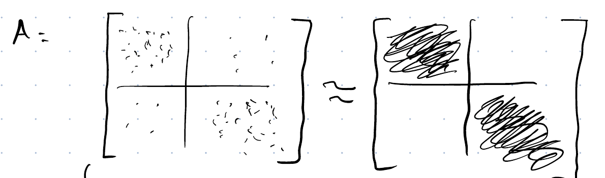
Two common choices of similarity:
\[A_{ij} = \begin{cases} \vx_i^{\,T} \vx_j \\[4pt] e^{\displaystyle -\frac{\norm{\vx_i - \vx_j}^2}{2\bandwidth^2}} \quad \textcolor{green}{\uparrow \text{scale}} \end{cases}\]
The second is the Gaussian kernel that we used for kernel smoothing in Non-Parametric Models, and \(\bandwidth\) plays the same role.
Compared with k-means, spectral clustering can follow a cluster of any shape. K-means assigns each point to the nearest center, so its clusters are the cells of a Voronoi diagram, which are convex. Spectral clustering never measures distance to a center in the input space. It asks only which points are connected to which, so a long curved band of points that are each close to their neighbors holds together even though its two ends are far apart. It does run k-means at the end, but on the eigenvector embedding rather than on the original coordinates, and the embedding has already straightened the band. Other ways to relax k-means’ assumption are to change the distance metric, to build the graph from each point’s nearest neighbors rather than from a kernel over every pair, or to fit a mixture of Gaussians, whose components are ellipses rather than Voronoi cells — a mixture-model view that Section 8.1 takes up.
Connecting each point to its \(k\) nearest neighbors — a \(k\) chosen independently of the number of clusters \(K\) — is the usual way to turn a set of points into a graph in the first place, and it makes the similarity matrix \(A\) sparse.
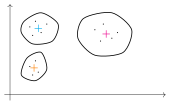
von Luxburg’s lectures cover:
GeeksforGeeks explains spectral clustering [11].
Both algorithms so far need \(K\) before they start. Agglomerative clustering does not. It begins with every point in its own cluster, repeatedly merges the two closest clusters, and stops only when one cluster holds everything — producing not a single partition but a nested family of them, one for every number of clusters from \(N\) down to \(1\). The record of which clusters merged, and at what height, is a dendrogram.
The algorithm needs a dissimilarity \(D(C_i,C_j)\) between clusters, built out of the dissimilarity \(d(x,x')\) between points. That construction is the linkage criterion, and given \(d\) it is the only choice the algorithm makes.
Single linkage takes the closest cross-cluster pair: \[D(C_i,C_j) = \min_{x \in C_i,\; x' \in C_j} d(x,x')\]
Complete linkage takes the farthest: \[D(C_i,C_j) = \max_{x \in C_i,\; x' \in C_j} d(x,x')\]
Average linkage takes the mean over all cross-cluster pairs: \[D(C_i,C_j) = \frac{1}{|C_i|\,|C_j|} \sum_{x \in C_i} \sum_{x' \in C_j} d(x,x')\]
Ward linkage reduces no set of pairwise distances at all. It asks how far the within-cluster sum of squares would rise if the two clusters merged: \[D(C_i,C_j) = \frac{|C_i|\,|C_j|}{|C_i| + |C_j|} \,\norm{\mean_i - \mean_j}_2^2\] where \(\mean_i\) is the mean of \(C_i\) [12]. That quantity is exactly the increase in \(\sum_k \sum_{x \in C_k}\norm{x - \mean_k}_2^2\) caused by the merge, so greedily merging the cheapest pair is a bottom-up descent on the k-means objective.
Ward’s heights therefore sit on a different scale from the other three: for two singletons it returns \(\tfrac{1}{2} d(x,x')^2\) rather than \(d(x,x')\). Keep that in mind when comparing heights across linkages.
We have four weather stations and a dissimilarity for every pair:
| W | X | Y | Z | |
|---|---|---|---|---|
| W | — | 0.12 | 0.30 | 0.50 |
| X | 0.12 | — | 0.24 | 0.46 |
| Y | 0.30 | 0.24 | — | 0.35 |
| Z | 0.50 | 0.46 | 0.35 | — |
Take average linkage. The smallest entry is \(d(W,X) = 0.12\), so W and X merge first, at height \(0.12\). Rebuild the table against the new cluster:
\[ \begin{aligned} D(W{+}X, Y) &= \frac{0.30 + 0.24}{2} \\ &= 0.27, \end{aligned} \qquad \begin{aligned} D(W{+}X, Z) &= \frac{0.50 + 0.46}{2} \\ &= 0.48 \end{aligned} \]
| W+X | Y | Z | |
|---|---|---|---|
| W+X | — | 0.27 | 0.48 |
| Y | 0.27 | — | 0.35 |
| Z | 0.48 | 0.35 | — |
Now \(0.27\) is smallest, so Y joins at that height. One distance remains, and it needs care:
\[ \begin{aligned} D(Y{+}W{+}X, Z) &= \frac{d(Y,Z) + d(W,Z) + d(X,Z)}{3} \\ &= \frac{0.35 + 0.50 + 0.46}{3} \\ &= \frac{1.31}{3} \\ &\approx 0.437 \end{aligned} \]
This is not \(\tfrac{1}{2}(0.35 + 0.48) = 0.415\). Average linkage averages over the original point pairs, so when we rebuild the table, the two old distances enter weighted by cluster size — one point in Y against two in W+X. Single and complete linkage have no such subtlety: a minimum of minima is a minimum, and a maximum of maxima is a maximum, whatever the cluster sizes.
Z joins last, at height \(\tfrac{1.31}{3} \approx 0.437\), and the dendrogram is complete.
A dendrogram is not a clustering; it is every clustering at once. Draw a horizontal line at height \(\cutheight\) and read off the branches it severs: that is the partition you get by refusing any merge costing more than \(\cutheight\). Cutting the tree of Section 5.2 at \(\cutheight = 0.3\) leaves \(\{W,X,Y\}\) and \(\{Z\}\), and cutting at \(\cutheight = 0.2\) leaves \(\{W,X\}\), \(\{Y\}\) and \(\{Z\}\). Asking for exactly \(K\) clusters is the same operation counted from the other end: stop the merge sequence with \(K\) clusters still standing.
That is the practical appeal. We choose the number of clusters after looking at the tree rather than before running the algorithm, and a tall gap between consecutive merge heights is the dendrogram’s version of the elbow.
Exercise 14 (Compare single and complete linkage on a line) Five points on the real line sit at \(0\), \(1\), \(2.5\), \(4.5\) and \(6.6\).
Cluster them by hand with agglomerative clustering and single linkage. Say which clusters merge at each step and at what height, draw the tree, and give the two clusters you get by stopping at \(K = 2\).
Exercise 15 (Compare single and complete linkage on a line (part 2)) Use the setup of Exercise 14.
Cluster them by hand with agglomerative clustering and complete linkage. Say which clusters merge at each step and at what height, draw the tree, and give the two clusters you get by stopping at \(K = 2\).
Exercise 16 (Compare single and complete linkage on a line (part 3)) Use the setup of Exercise 14.
Do the two linkages agree?
Exercise 17 (Build a dendrogram by hand with average linkage) Five points have the pairwise distances below.
| A | B | C | D | E | |
|---|---|---|---|---|---|
| A | — | 1.0 | 3.0 | 4.4 | 9.2 |
| B | 1.0 | — | 2.0 | 3.4 | 8.2 |
| C | 3.0 | 2.0 | — | 1.4 | 6.2 |
| D | 4.4 | 3.4 | 1.4 | — | 4.8 |
| E | 9.2 | 8.2 | 6.2 | 4.8 | — |
Run agglomerative clustering with average linkage by hand. At each step, say which two clusters merge and at what height, and rebuild the distance table against the new cluster.
Exercise 18 (Build a dendrogram by hand with average linkage (part 2)) Use the setup of Exercise 17.
Draw the dendrogram.
# Each row of `merge` joins two items, a negative index for a point
# and a positive index for the cluster made at that earlier row.
merge_rows <- five_tree$merge
heights <- five_tree$height
leaf_x <- match(seq_along(five_tree$order), five_tree$order)

item_x <- function(item, cluster_x) {
  if (item < 0) leaf_x[-item] else cluster_x[item]
}
item_height <- function(item) if (item < 0) 0 else heights[item]

cluster_x <- numeric(nrow(merge_rows))
bars <- list()
for (i in seq_len(nrow(merge_rows))) {
  left <- merge_rows[i, 1]
  right <- merge_rows[i, 2]
  xs <- c(item_x(left, cluster_x), item_x(right, cluster_x))
  cluster_x[i] <- mean(xs)
  bars[[i]] <- data.frame(
    x = c(xs[1], xs[1], xs[2]),
    xend = c(xs[1], xs[2], xs[2]),
    y = c(item_height(left), heights[i], item_height(right)),
    yend = c(heights[i], heights[i], heights[i])
  )
}
bars <- do.call(rbind, bars)
merge_labels <- data.frame(
  x = cluster_x,
  y = heights,
  label = format(round(heights, 1), nsmall = 1)
)

ggplot2::ggplot() +
  ggplot2::geom_segment(
    data = bars,
    ggplot2::aes(x = x, xend = xend, y = y, yend = yend)
  ) +
  ggplot2::geom_text(
    data = merge_labels,
    ggplot2::aes(x = x, y = y, label = label),
    hjust = -0.3,
    vjust = -0.5
  ) +
  ggplot2::scale_y_continuous(expand = ggplot2::expansion(mult = c(0.02, 0.1))) +
  ggplot2::scale_x_continuous(
    breaks = seq_along(five_tree$order),
    labels = five_tree$labels[five_tree$order]
  ) +
  ggplot2::labs(x = NULL, y = "merge height") +
  ggplot2::theme_minimal() +
  ggplot2::theme(panel.grid.major.x = ggplot2::element_blank())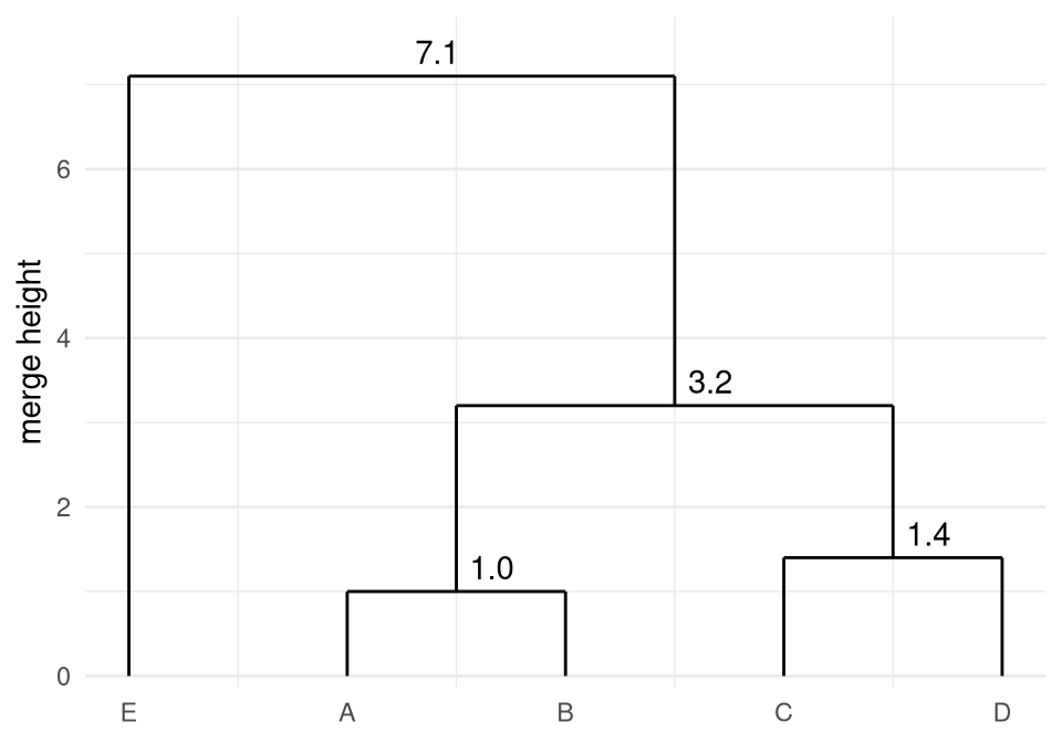
Exercise 19 (Cut the dendrogram to get a chosen number of clusters) For the dendrogram of Exercise 18, which heights \(\cutheight\) give two clusters?
Exercise 20 (Cut the dendrogram to get a chosen number of clusters (part 2)) Use the setup of Exercise 19.
List the two clusters given by a cut in the range of heights found in Exercise 19.
Exercise 21 (Cut the dendrogram to get a chosen number of clusters (part 3)) Use the setup of Exercise 19.
For the dendrogram of Exercise 18, which heights \(\cutheight\) give three clusters?
Exercise 22 (Cut the dendrogram to get a chosen number of clusters (part 4)) Use the setup of Exercise 19.
List the three clusters given by a cut in the range of heights found in Exercise 21.
Exercise 23 (Cut the dendrogram to get a chosen number of clusters (part 5)) Use the setup of Exercise 19.
Does the dendrogram favor two clusters (Exercise 19) or three (Exercise 21), and why?
The four criteria differ only in how height reduces a pair of clusters, so one implementation can run all four over the same seven points. The code prints each merge as the cluster it produced followed by the height it happened at.
import itertools
import math

X = [(0.0, 0.0), (0.9, 0.5), (2.1, 0.1), (3.2, 0.6),
     (6.0, 3.0), (6.8, 3.5), (9.2, 0.2)]
labels = "ABCDEFG"

def height(ci, cj, linkage):
    if linkage == "ward":                # rise in within-cluster sum of squares
        mi = [sum(X[k][t] for k in ci) / len(ci) for t in (0, 1)]
        mj = [sum(X[k][t] for k in cj) / len(cj) for t in (0, 1)]
        gap = sum((mi[t] - mj[t]) ** 2 for t in (0, 1))
        return len(ci) * len(cj) / (len(ci) + len(cj)) * gap
    d = [math.dist(X[a], X[b]) for a in ci for b in cj]
    if linkage == "single":
        return min(d)
    if linkage == "complete":
        return max(d)
    return sum(d) / len(d)

def agglomerate(linkage):
    clusters = [[i] for i in range(len(X))]
    steps = []
    while len(clusters) > 1:
        pairs = list(itertools.combinations(range(len(clusters)), 2))
        a, b = min(pairs, key=lambda p: height(clusters[p[0]], clusters[p[1]], linkage))
        h = height(clusters[a], clusters[b], linkage)
        merged = sorted(clusters[a] + clusters[b])
        steps.append("".join(labels[i] for i in merged) + "@" + str(round(h, 3)))
        clusters = [c for k, c in enumerate(clusters) if k not in (a, b)] + [merged]
    print(linkage, " ".join(steps))

for name in ["single", "complete", "average", "ward"]:
    agglomerate(name)
single EF@0.943 AB@1.03 CD@1.208 ABCD@1.265 ABCDEF@3.688 ABCDEFG@4.08
complete EF@0.943 AB@1.03 CD@1.208 ABCD@3.256 EFG@4.252 ABCDEFG@9.202
average EF@0.943 AB@1.03 CD@1.208 ABCD@2.231 EFG@4.166 ABCDEFG@6.354
ward EF@0.445 AB@0.53 CD@0.73 ABCD@4.85 EFG@11.428 ABCDEFG@63.745X <- matrix(c(0.0, 0.0, 0.9, 0.5, 2.1, 0.1, 3.2, 0.6,
6.0, 3.0, 6.8, 3.5, 9.2, 0.2), ncol = 2, byrow = TRUE)
labels <- strsplit("ABCDEFG", "")[[1]]
height <- function(ci, cj, linkage) {
if (linkage == "ward") { # rise in within-cluster sum of squares
mi <- colMeans(X[ci, , drop = FALSE])
mj <- colMeans(X[cj, , drop = FALSE])
gap <- sum((mi - mj)^2)
return(length(ci) * length(cj) / (length(ci) + length(cj)) * gap)
}
d <- as.vector(outer(ci, cj, Vectorize(function(a, b) sqrt(sum((X[a, ] - X[b, ])^2)))))
if (linkage == "single") return(min(d))
if (linkage == "complete") return(max(d))
mean(d)
}
agglomerate <- function(linkage) {
clusters <- lapply(seq_len(nrow(X)), function(i) i)
steps <- character(0)
while (length(clusters) > 1) {
pairs <- combn(length(clusters), 2)
hs <- apply(pairs, 2, function(p) height(clusters[[p[1]]], clusters[[p[2]]], linkage))
k <- which.min(hs)
a <- pairs[1, k]; b <- pairs[2, k]
merged <- sort(c(clusters[[a]], clusters[[b]]))
steps <- c(steps, paste0(paste(labels[merged], collapse = ""), "@", round(hs[k], 3)))
clusters <- c(clusters[-c(a, b)], list(merged))
}
cat(linkage, " ", paste(steps, collapse = " "), "\n", sep = "")
}
for (name in c("single", "complete", "average", "ward")) agglomerate(name)single EF@0.943 AB@1.03 CD@1.208 ABCD@1.265 ABCDEF@3.688 ABCDEFG@4.08
complete EF@0.943 AB@1.03 CD@1.208 ABCD@3.256 EFG@4.252 ABCDEFG@9.202
average EF@0.943 AB@1.03 CD@1.208 ABCD@2.231 EFG@4.166 ABCDEFG@6.354
ward EF@0.445 AB@0.53 CD@0.73 ABCD@4.85 EFG@11.428 ABCDEFG@63.745X = [(0.0, 0.0), (0.9, 0.5), (2.1, 0.1), (3.2, 0.6),
(6.0, 3.0), (6.8, 3.5), (9.2, 0.2)];
labels = "ABCDEFG";
function height(ci, cj, linkage)
if linkage == "ward" # rise in within-cluster sum of squares
mi = (sum(X[k][1] for k in ci) / length(ci), sum(X[k][2] for k in ci) / length(ci))
mj = (sum(X[k][1] for k in cj) / length(cj), sum(X[k][2] for k in cj) / length(cj))
gap = (mi[1] - mj[1])^2 + (mi[2] - mj[2])^2
return length(ci) * length(cj) / (length(ci) + length(cj)) * gap
end
d = [sqrt((X[a][1] - X[b][1])^2 + (X[a][2] - X[b][2])^2) for a in ci for b in cj]
linkage == "single" && return minimum(d)
linkage == "complete" && return maximum(d)
return sum(d) / length(d)
end;
function agglomerate(linkage)
clusters = [[i] for i in 1:length(X)]
steps = String[]
while length(clusters) > 1
pairs = [(i, j) for i in 1:length(clusters) for j in (i + 1):length(clusters)]
hs = [height(clusters[p[1]], clusters[p[2]], linkage) for p in pairs]
k = argmin(hs)
a, b = pairs[k]
merged = sort(vcat(clusters[a], clusters[b]))
push!(steps, join(labels[i] for i in merged) * "@" * string(round(hs[k], digits = 3)))
clusters = [c for (i, c) in enumerate(clusters) if i != a && i != b]
push!(clusters, merged)
end
println(linkage, " ", join(steps, " "))
end;
for name in ["single", "complete", "average", "ward"]
agglomerate(name)
endsingle EF@0.943 AB@1.03 CD@1.208 ABCD@1.265 ABCDEF@3.688 ABCDEFG@4.08
complete EF@0.943 AB@1.03 CD@1.208 ABCD@3.256 EFG@4.252 ABCDEFG@9.202
average EF@0.943 AB@1.03 CD@1.208 ABCD@2.231 EFG@4.166 ABCDEFG@6.354
ward EF@0.445 AB@0.53 CD@0.73 ABCD@4.85 EFG@11.428 ABCDEFG@63.745All four agree on the first four merges. The pairs AB, CD and EF are tight, and ABCD follows. They differ on the fifth merge, and the difference is structural rather than numerical. Single linkage joins ABCD to EF, because the closest single pair between them, \(d(D,E) = 3.688\), beats the \(4.080\) separating F from G. The other three measure the whole spread instead, and by that measure G is the better partner for EF. So cutting at \(K=2\) gives \(\{A,\ldots,F\}\) and \(\{G\}\) under single linkage but \(\{A,B,C,D\}\) and \(\{E,F,G\}\) under the other three, on identical data with an identical \(d\). Single linkage’s willingness to follow one short hop at a time lets it trace out non-convex shapes, and equally lets a single bridging point chain two clusters together.
Exercise 24 (Recover two interleaved crescents) A data set has 300 points in the plane, forming two interleaved crescents (the “two moons” shape) with a clear gap between them and little noise. You want the two crescents back as two clusters. Which would you expect to work: \(K\)-means with \(K = 2\), or single-link agglomerative clustering cut at two clusters?
Exercise 25 (Recover two interleaved crescents (part 2)) Use the setup of Exercise 24.
Say what single-link agglomerative clustering does to the crescents, and why.
Exercise 26 (Recover two interleaved crescents (part 3)) Use the setup of Exercise 24.
Say what \(K\)-means with \(K = 2\) does to the crescents, and why.
GeeksforGeeks explains:
Clustering assigns each point a label. The other common unsupervised task is to re-describe every point in fewer dimensions [16].
A second motive for reducing \(D\) has nothing to do with storage. As dimension grows, distances concentrate: the gap between a point’s nearest and farthest neighbours shrinks relative to the typical distance between points, so “nearest” carries less and less information. Under broad conditions on the data distribution that relative gap converges to zero, and the effect is measurable in as few as 10 to 15 dimensions [17].
K-means, spectral clustering and hierarchical clustering all compare distances and do nothing else, so they degrade together. The assignment step of k-means shows it most plainly. If every centroid is nearly equidistant from a point, the \(\argmin\) is settled by noise, and a small change to the data or to the initialization produces a completely different clustering from the same objective.
Two responses are standard. Reduce the dimension before clustering. Or change the metric: within the Minkowski family, smaller \(p\) concentrates more slowly, so Manhattan preserves more contrast than Euclidean at the same dimension [18], and cosine similarity discards magnitude entirely, which helps when the structure worth finding lies in a vector’s direction rather than its length.
GeeksforGeeks explains the curse of dimensionality [19].
We want \(\mX_r \approx \mX\) with \(\operatorname{rank}(\mX_r) = r\): a low-rank matrix is a simple matrix. Rank is the number of linearly independent columns or rows, equivalently the smallest number of rank-1 matrices that add up to \(\mX\). The word “smallest” is essential: any rank-1 matrix can be written as a sum of three rank-1 matrices, so without it the count would not be a single number.
The singular value decomposition, or SVD for short, writes \(\mX\) as exactly such a sum:
\[ \begin{aligned} \mX &= U S \tp{V} \\ &= \sum_{i=1}^{\operatorname{rank}(\mX)} \underbrace{\vu_i \singval_i \vv_i^{\,\top}}_{\text{rank-1 matrix}} \qquad \textcolor{green}{\singval_1 \geq \singval_2 \geq \dots \geq \singval_{\operatorname{rank}(\mX)}} \end{aligned} \]
Because the singular values are ordered, truncating the sum keeps the largest pieces:
\[\mX_r = \sumto{i}{r} \singval_i\, \underbrace{\vu_i \vv_i^{\,\top}}_{\textcolor{orange}{\text{rank-1 term}}}\]
This truncation is optimal: no other matrix of rank \(r\) or less is closer to \(\mX\).
\[\mX_r \text{ solves } \min_{\substack{Z \\ \operatorname{rank}(Z) \,\leq\, r}}\norm{\mX - Z}_F\]
Here \(\norm{A}_F = \sqrt{\sum_{i,j} A_{ij}^2}\) is the Frobenius norm, the entrywise analogue of the Euclidean vector norm. The constraint is \(\operatorname{rank}(Z) \leq r\) rather than \(= r\), since that is the set the truncation minimizes over.
GeeksforGeeks explains the singular value decomposition [20].
Principal component analysis, or PCA for short, is that same truncation applied to the centered data [21]. Write
\[\cent{\mX} = \mX - \vone\,\bar{\vx}^{\,\top}, \qquad \bar{\vx} = \avgiN x_{(i)}\]
for the data matrix with each column’s mean subtracted, and take its SVD \(\cent{\mX} = U S \tp{V}\). Then
\[\cent{\mX} \approx \sumto{i}{r} \singval_i\, \vu_i \vv_i^{\,\top}\]
is the best rank-\(r\) approximation to the centered data. Its directions \(\vv_i\) are the loadings, or principal components, and the \(\singval_i \vu_i\) are the scores.
Centering is not a detail to skip. If we run the SVD on \(\mX\) itself, the leading singular direction is pulled toward the mean of the data, so \(\vv_1\) would describe where the data sits rather than how it varies — the one thing we ask PCA to describe.
We can arrive at the same \(\vv_i\) a second way, and this way gives the phrase “variance explained” its meaning. Instead of asking for the best rank-\(r\) approximation, ask for the single direction along which the data varies most.
Project the centered rows onto a unit vector \(\vu\). The projections \(t_i = \tp{\cent{\vx}_{(i)}} \vu\) have mean zero, because we centered the data, so their variance is
\[\avgiN t_i^2 = \vu^{\,\top} \hcovmat \, \vu, \qquad \hcovmat = \frac{1}{N} \tp{\cent{\mX}} \cent{\mX}\]
where \(\hcovmat\) is the sample covariance matrix: the estimate, from these \(N\) rows, of the population’s variance matrix \(\covmat\). Maximizing that subject to \(\norm{\vu}_2 = 1\) gives the Lagrangian \(\vu^{\,\top} \hcovmat \vu - \lagmult(\vu^{\,\top}\vu - 1)\), whose stationary condition is
\[\hcovmat \, \vu = \eigval \vu\]
So \(\vu\) must be an eigenvector of \(\hcovmat\), and since \(\vu^{\,\top} \hcovmat \vu = \eigval\) at any such \(\vu\), the maximizing choice is the one with the largest eigenvalue. Requiring the next direction to be orthogonal to the first and repeating gives the second eigenvector, and so on down.
This is the same answer as before, not a rival one. From \(\cent{\mX} = US\tp{V}\),
\[ \begin{aligned} \tp{\cent{\mX}} \cent{\mX} &= V S \stprod{U} S \tp{V} \\ &= V S^2 \tp{V} \end{aligned} \qquad\Longrightarrow\qquad \hcovmat = V \paren{\tfrac{1}{N} S^2} \tp{V} \]
The eigenvectors of \(\hcovmat\) are exactly the right singular vectors \(\vv_i\), and the variance along \(\vv_i\) is \(\singval_i^2 / N\). Dividing by the total,
\[\frac{\singval_i^2 / N}{\sum_j \singval_j^2 / N} = \frac{\singval_i^2}{\sum_j \singval_j^2}\]
is the fraction of the total variance that component \(i\) accounts for, the quantity usually called the explained variance ratio.
Pythagoras explains why the two derivations agree. For a unit \(\vu\), each centered point splits into its projection and what is left over,
\[\norm{\cent{\vx}_{(i)}}_2^2 = t_i^2 +\norm{\cent{\vx}_{(i)} - t_i \vu}_2^2\]
and summing over \(i\) gives \(\norm{\cent{\mX}}_F^2 = \sum_i t_i^2 + \sum_i\norm{\cent{\vx}_{(i)} - t_i \vu}_2^2\). The left side does not depend on \(\vu\) at all. So maximizing the projected variance is the same as minimizing the squared reconstruction error. Pearson fit the line of closest fit to a cloud of points [22]. Hotelling later developed principal components as the directions of greatest variance [23]. The two formulations therefore describe one method.
Starmer works through principal component analysis [24] step by step.
GeeksforGeeks explains principal component analysis [25].
PCA is the SVD of the centered matrix, so the implementation is two lines and the interesting part is what happens when you get one of them wrong. Each of the three tabs runs it twice: once properly, and once on the uncentered \(\mX\), where we deliberately place the cloud a long way from the origin.
import numpy as np

rng = np.random.default_rng(0)
n = 200
t = rng.normal(scale=3.0, size=n)
X = np.column_stack([t, 2 * t]) + rng.normal(scale=0.3, size=(n, 2))
X = X + np.array([50.0, 10.0])          # park the cloud away from the origin

Xc = X - X.mean(axis=0)                 # the one line that makes it PCA
U, S, Vt = np.linalg.svd(Xc, full_matrices=False)

print("explained:", (S ** 2 / (S ** 2).sum()).round(4))
explained: [0.9978 0.0022]print("v1:", Vt[0].round(3))v1: [-0.441 -0.898]print("rank-1 error:",
round(float(np.linalg.norm(Xc - S[0] * np.outer(U[:, 0], Vt[0]))), 3))rank-1 error: 4.326V_uncentered = np.linalg.svd(X, full_matrices=False)[2]
print("uncentered v1:", V_uncentered[0].round(3),
"| mean direction:", (X.mean(0) / np.linalg.norm(X.mean(0))).round(3))uncentered v1: [-0.979 -0.205] | mean direction: [0.98 0.198]set.seed(0)
n <- 200
z <- rnorm(n, sd = 3)
X <- cbind(z, 2 * z) + matrix(rnorm(2 * n, sd = 0.3), ncol = 2)
X <- sweep(X, 2, c(50, 10), "+") # park the cloud away from the origin
Xc <- scale(X, center = TRUE, scale = FALSE) # the one line that makes it PCA
s <- svd(Xc)
cat("explained:", round(s$d^2 / sum(s$d^2), 4), "\n")explained: 0.9977 0.0023 v1: -0.445 -0.895 rank-1 error: 4.196 uncentered v1: -0.979 -0.202 | mean direction: 0.981 0.195 using Random, LinearAlgebra, Statistics
Random.seed!(0);
n = 200;
z = 3 .* randn(n);
X = [z 2 .* z] .+ 0.3 .* randn(n, 2);
# park the cloud away from the origin
X = X .+ [50.0 10.0];
# the one line that makes it PCA
Xc = X .- mean(X, dims = 1);
U, S, V = svd(Xc);
println("explained: ", round.(S .^ 2 ./ sum(S .^ 2), digits = 4))explained: [0.9982, 0.0018]println("v1: ", round.(V[:, 1], digits = 3))v1: [0.452, 0.892]println("rank-1 error: ",
round(norm(Xc - S[1] * U[:, 1] * V[:, 1]'), digits = 3))rank-1 error: 4.033
V_uncentered = svd(X).V;
mu = vec(mean(X, dims = 1));
println("uncentered v1: ", round.(V_uncentered[:, 1], digits = 3),
        " | mean direction: ", round.(mu ./ norm(mu), digits = 3))
uncentered v1: [-0.977, -0.215] | mean direction: [0.978, 0.207]# What the three tabs print, gathered for the prose, with the claims it
# makes in words checked here.
jl <- function(expr) JuliaCall::julia_eval(expr)
pca <- list(
py = list(explained = py$S^2 / sum(py$S^2), v1 = py$Vt[1, ],
unc_v1 = py$V_uncentered[1, ], X = py$X),
r = list(explained = s$d^2 / sum(s$d^2), v1 = s$v[, 1],
unc_v1 = v_uncentered, X = X),
jl = list(explained = jl("S .^ 2 ./ sum(S .^ 2)"), v1 = jl("V[:, 1]"),
unc_v1 = jl("V_uncentered[:, 1]"), X = jl("X"))
)
truth <- c(1, 2) / sqrt(5)
for (p in pca) {
mu <- colMeans(p$X)
mean_dir <- mu / sqrt(sum(mu^2))
d_unc <- svd(p$X)$d
stopifnot(
max(abs(abs(p$v1) - truth)) < 0.01,
max(abs(abs(p$unc_v1) - mean_dir)) < 0.01,
d_unc[1]^2 / sum(d_unc^2) > 0.99
)
}
explained_pct <- unique(vapply(pca, function(p) round(100 * p$explained[1], 1),
numeric(1)))
explained_text <- if (length(explained_pct) == 1) {
sprintf("all three put $%s\\%%$", explained_pct)
} else {
sprintf("each puts between $%s\\%%$ and $%s\\%%$",
min(explained_pct), max(explained_pct))
}
# Which sign each library returns is an implementation detail, so the prose
# reports whatever the three returned on this render.
v1_signs <- vapply(pca, function(p) sign(p$v1[which.max(abs(p$v1))]),
numeric(1))
sign_text <- if (length(unique(v1_signs)) > 1) {
"The signs do not match."
} else {
"The signs happen to match on this render, and nothing guarantees they will."
}
fmt_v <- function(v, digits = 3) {
paste0("(", paste(formatC(v, format = "f", digits = digits, flag = "+"),
collapse = ", "), ")")
}
py_mu <- colMeans(pca$py$X)We built the data to vary along \((1,2)\), whose unit vector is \((0.447, 0.894)\). All three recover it to within \(0.01\), and all three put \(99.8\%\) of the variance on that one component. The noise we added to each coordinate is isotropic rather than perpendicular to the line, so it lands partly along the line and partly across it; the second singular value measures the part that lands across.
Two things in the printed output matter more than the agreement.
The signs are arbitrary. The signs do not match. Python returns \(\vv_1 = (-0.441, -0.898)\) and R returns \((-0.445, -0.895)\), each drawing its own sample; Julia returns \((+0.452, +0.892)\). All three are correct. If \(\vu_i \singval_i \vv_i^{\,\top}\) is a term of the decomposition then so is \((-\vu_i)\singval_i(-\vv_i)^{\,\top}\), so the SVD fixes the axis and not the direction along it, and which one a library returns is a detail of its implementation. Never read a sign, or the sign of a score, as meaning anything; compare \(|\vv_1|\), or fix the convention yourself by flipping so that the largest-magnitude entry is positive.
Skipping the centering does not degrade the answer, it replaces it. The uncentered run returns \(\vv_1 \approx (-0.98, -0.21)\) in Python, against a mean direction of \(\approx (+0.98, +0.20)\): the same axis, and nothing to do with \((0.447, 0.894)\). R and Julia each land on the axis of their own mean direction, to within \(0.01\). The leading component has stopped describing how the data varies and started describing where it is. Nothing warns you — it still reports over \(99\%\) of variance explained, because the mean is genuinely the largest thing in an uncentered matrix. So Section 6.3 insists centering is not a detail to skip, and placing a cloud far from the origin once lets you see it happen.
Exercise 27 (Find the main directions of variation in car specifications) The Auto data of James et al. [26] describe 392 cars. Download auto.csv to load it in Python or R. Take five columns: mpg, displacement, horsepower, weight and acceleration. These are measured in different units, so standardize each column to mean 0 and standard deviation 1. Then run PCA on the standardized matrix with the SVD. Before you run it, say how many components you expect to need to describe most of the variation, and which columns you expect to load together.
Exercise 28 (Find the main directions of variation in car specifications (part 2)) Use the setup of Exercise 27.
Report the share of variance each component explains.
Exercise 29 (Find the main directions of variation in car specifications (part 3)) Use the setup of Exercise 27.
Report the loadings of the first component.
Exercise 30 (Find the main directions of variation in car specifications (part 4)) Use the setup of Exercise 27.
Plot each car by its first two component scores, using a different symbol for each origin (1 is American, 2 is European and 3 is Japanese).
library(ggplot2)
scores <- Zc %*% cbind(flip * pca_cars$v[, 1], pca_cars$v[, 2])
scores_df <- tibble::tibble(
  pc1 = scores[, 1],
  pc2 = scores[, 2],
  weight = cars$weight,
  origin = factor(cars$origin, levels = 1:3,
                  labels = c("American", "European", "Japanese"))
)
ggplot(scores_df, aes(pc1, pc2, shape = origin, colour = weight)) +
  geom_point(size = 2) +
  scale_colour_viridis_c(labels = scales::label_comma()) +
  scale_shape_manual(values = c(American = 1, European = 2, Japanese = 3)) +
  labs(x = "component 1 score", y = "component 2 score", shape = NULL,
       colour = "weight (lb)") +
  theme(legend.position = "bottom")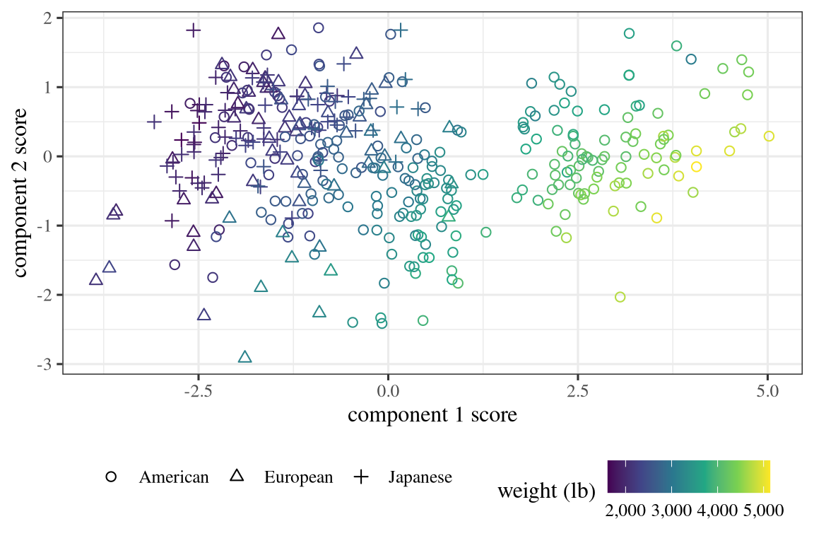
Exercise 31 (Find the main directions of variation in car specifications (part 5)) Use the setup of Exercise 27.
How many components are needed to describe most of the variation? Compare with the number you expected before running PCA.
Exercise 32 (Find the main directions of variation in car specifications (part 6)) Use the setup of Exercise 27.
Which columns load together? Compare with the columns you expected to load together.
Exercise 33 (Find the main directions of variation in car specifications (part 7)) Use the setup of Exercise 27.
Why must the columns be standardized before PCA here?
Goal is to estimate \(p(x)\), the probability density function (pdf) of the data
This is unsupervised, probabilistic, and generative
Why?
Understand the structure of the data / gain insight
Anomaly detection
Generate new data (see image generation models)
We are going to focus on Gaussian and Gaussian Mixture Model distributions, as they are the commonly used, flexible, and easy to understand
The probability behind this section lives in Probability for Data Science, which we call “pds” below. This chapter uses that material rather than re-deriving it:
the normal distribution and its mean and variance
the multivariate normal distribution (MVN for short), \(\operatorname{N}_D(\mean, \covmat)\), whose mean is \(\mean\) and variance matrix is \(\covmat\)
the variance matrix, whose elements are the pairwise covariances, and which is always symmetric and positive semidefinite
For reference, the MVN density over \(x \in \reals^D\) is \[p(x) = \frac{1}{\sqrt{(2\pi)^D |\covmat|}} \expf{-\frac{1}{2} \underbrace{(x-\mean)^T \covmat^{-1} (x-\mean)}_{\text{(Squared) Mahalanobis distance } d(x,\mean)}}\] with \(\covmat\) positive definite, so that \(\covmat^{-1}\) and \(|\covmat|\) exist and \(|\covmat| > 0\): \(|\covmat|\) is the product of \(\covmat\)’s eigenvalues, which are all positive.
Why the off-diagonal entries matter: two four-point datasets with the same per-coordinate variances can have variance matrices that differ only in the sign of the covariance, tilting their point clouds in opposite directions.
The density decreases with the Mahalanobis distance from \(\mean\) (proof):
special cases: \(\covmat = I\) gives Euclidean distance (spheres), \(\covmat = cI\) a rescaled one, and a diagonal \(\covmat\) axis-aligned ellipsoids
in general, ellipsoids aligned with the eigenvectors of \(\covmat\), with widths set by the eigenvalues
a diagonal \(\covmat\) means independent normal components; for an MVN, uncorrelated components are independent
\(\covmat^{-1}\) is sometimes called the precision or concentration matrix; it is positive definite too.
Exercise 34 (Sketch the one-standard-deviation ellipse of a Gaussian) Each of the following covariance matrices defines a 2-dimensional Gaussian with mean \(\mean = (0, 0)^T\):
\[ \covmat_1 = \begin{pmatrix} 4 & 0 \\ 0 & 1 \end{pmatrix}, \quad \covmat_2 = \begin{pmatrix} 1 & 0.5 \\ 0.5 & 1 \end{pmatrix}, \quad \covmat_3 = \begin{pmatrix} 1 & -0.5 \\ -0.5 & 1 \end{pmatrix}, \quad \covmat_4 = \begin{pmatrix} 1 & 0.9 \\ 0.9 & 1 \end{pmatrix}. \]
For each, sketch the set of points whose Mahalanobis distance from \(\mean\) is \(1\) (the one-standard-deviation ellipse).
Solution 34. The set of points at Mahalanobis distance \(1\) is \(\{x : (x - \mean)^T \covmat^{-1} (x - \mean) = 1\}\). Its axes point along the eigenvectors of \(\covmat\).
\(\covmat_1\) is diagonal, so the axes are the coordinate axes.
\(\covmat_2\) has a positive covariance. The ellipse tilts along the line \(x_2 = x_1\).
\(\covmat_3\) has a negative covariance, so the long axis now lies along \((1, -1)^T\). A negative covariance tilts the ellipse the other way.
\(\covmat_4\) tilts the same way as \(\covmat_2\). It is a long thin ellipse: the strong covariance says the two coordinates almost move together.
The code below draws the four ellipses in Figure 5.
covs <- list(
  Sigma_1 = matrix(c(4, 0, 0, 1), 2),
  Sigma_2 = matrix(c(1, 0.5, 0.5, 1), 2),
  Sigma_3 = matrix(c(1, -0.5, -0.5, 1), 2),
  Sigma_4 = matrix(c(1, 0.9, 0.9, 1), 2)
)

# Points on the unit circle, mapped to the one-sd ellipse by the matrix square
# root of Sigma: Sigma = V diag(lambda) V^T, so the map is V diag(sqrt(lambda)).
theta <- seq(0, 2 * pi, length.out = 200)
circle <- rbind(cos(theta), sin(theta))
ellipse_points <- function(S) {
  e <- eigen(S)
  t(e$vectors %*% diag(sqrt(e$values)) %*% circle)
}

op <- par(mfrow = c(1, 4), mar = c(3, 3, 2, 0.5))
for (i in seq_along(covs)) {
  xy <- ellipse_points(covs[[i]])
  plot(xy, type = "l", asp = 1, xlim = c(-2.2, 2.2), ylim = c(-2.2, 2.2),
       xlab = "x1", ylab = "x2", main = names(covs)[i])
  abline(h = 0, v = 0, col = "grey80")
}
par(op)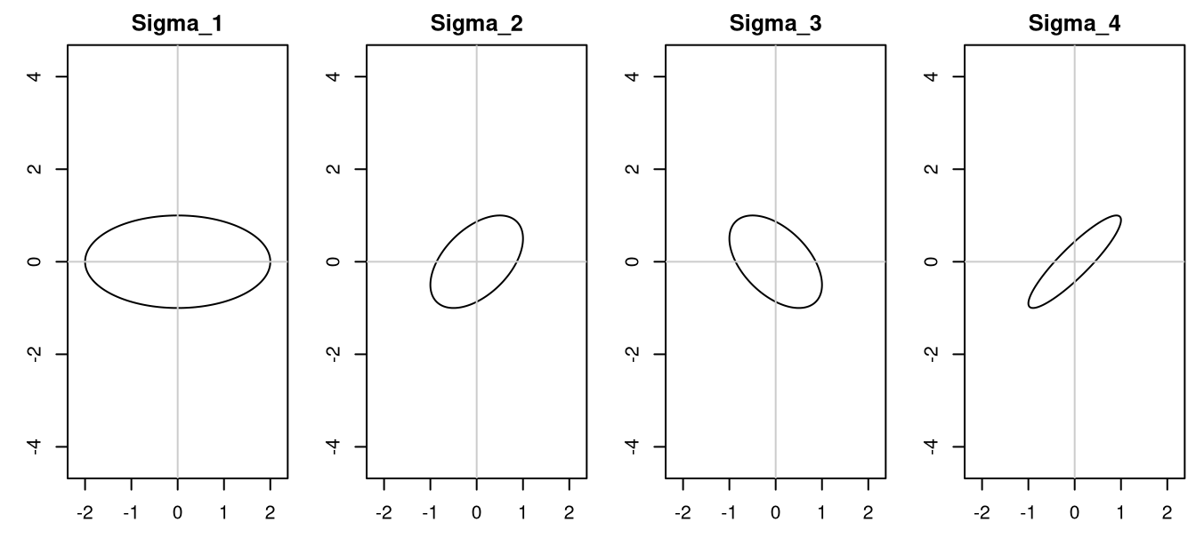
Exercise 35 (Sketch the one-standard-deviation ellipse of a Gaussian (part 2)) Use the setup of Exercise 34.
For each ellipse, mark its two axes and say how long each is.
Exercise 36 (Rank points by Mahalanobis distance) A Gaussian has mean \(\mean = (0, 0)^T\) and covariance matrix \(\covmat = \begin{pmatrix} 1 & 0.8 \\ 0.8 & 1 \end{pmatrix}\). Consider the points \(P = (1, 1)^T\), \(Q = (1, -1)^T\) and \(R = (2, 2)^T\).
Order them from closest to farthest from \(\mean\) by Euclidean distance.
Exercise 37 (Rank points by Mahalanobis distance (part 2)) Use the setup of Exercise 36.
Order them from closest to farthest from \(\mean\) by Mahalanobis distance.
Exercise 38 (Rank points by Mahalanobis distance (part 3)) Use the setup of Exercise 36.
Why do the two orders disagree?
Given a dataset \(\mathcal{X} = \{x_{(1)},\ldots,x_{(N)}\}\), how do we estimate \(\mean\) and \(\covmat\)?
We solve the following optimization problem (maximize likelihood): \[\begin{aligned} \argmax_{\mean,\covmat} p(\mathcal{X};\mean,\covmat) &= \argmax_{\mean,\covmat} \prod_{i=1}^N p(x_{(i)};\mean,\covmat) \\ &= \argmax_{\mean,\covmat} \ln \prod_{i=1}^N p(x_{(i)};\mean,\covmat) \\ &= \argmax_{\mean,\covmat} \sumiN \ln p(x_{(i)};\mean,\covmat) \end{aligned}\]
To solve it:
The solution is: \[\hmean = \avgiN x_{(i)}, \quad \hcovmat = \avgiN (x_{(i)} - \hmean)(x_{(i)} - \hmean)^T\]
This is the maximum likelihood estimate (MLE) for \(\mean\) and \(\covmat\)
Works well because many pdfs are log-concave, including normal distributions
Exercise 39 (Compute the maximum likelihood mean and covariance) Three points in the plane are \(x_{(1)} = (1, 2)^T\), \(x_{(2)} = (3, 0)^T\) and \(x_{(3)} = (5, 4)^T\). Compute the maximum likelihood estimate \(\hmean\) of the mean of a 2-dimensional Gaussian fit to them, by hand.
Exercise 40 (Compute the maximum likelihood mean and covariance (part 2)) Use the setup of Exercise 39.
Compute the maximum likelihood estimate \(\hcovmat\) of the covariance matrix of the same Gaussian, by hand.
Gaussians are useful, but they are unimodal
Often a population is made up of distinct sub-populations
We can model the overall population as a mixture of subpopulations - this is a mixture model \[p_{mix}(x) = \sumto{c}{M} w_c p_c(x)\]
\(w_1,\ldots,w_M\) are the mixture weights, non-negative, sum to one
pds covers the probability of mixtures: the two-stage construction, the mixture mean, and which component an observation came from, with a worked two-component example
When each model in the mixture is Gaussian, we call it a Gaussian mixture model (GMM for short)
With large enough \(M\), a GMM approximates any continuous density on \(\reals^d\) arbitrarily well: a narrow Gaussian behaves like a smoothed point mass, so a weighted sum of them is a smoothed histogram, and refining the histogram refines the fit. The claim is about the limit, not about exact representation at any finite \(M\)
The underlying generative process for a GMM is
Pick a sub-population (also called a component) according to \(w\) (also written \(P(c)\))
Sample from the Gaussian with \(\mean_{(c)}\) and covariance matrix \(\covmat_{(c)}\)
Repeat
Each draw has the mixture density \(p_{mix}\) (why).
GeeksforGeeks explains Gaussian mixture models [27].
The University of Washington’s CSE 446 slides cover Gaussian mixture models [5], Lecture 25.
GMM data log likelihood: \[\log P(\mathcal{X}|\param) = \sumiN \ln \paren{ \sumto{c}{M} w_c p(x_{(i)};\mean_{(c)},\covmat_{(c)}) }\]
This is hard to maximize directly. Taking the gradient is very difficult because the sum is inside the log.
Some variables are missing: which component generated each datapoint (\(z_{(i)} \in \reals^M\))
If we knew \(z_{(i)}\), the problem would be easy to solve
Here \(N_c = \sum_i z_{(i)c}\) is the number of points assigned to component \(c\) — a whole number, because each \(z_{(i)}\) is one-hot.
This simply takes the single MVN equations and applies them to each sub-population of the data, and then sets the \(w\) to the proportion of the data in that sub-population.
Unfortunately, we do not know \(z_{(i)}\).
But that doesn’t mean all components are equally likely to have generated each point
Picture two well-separated components with a point sitting deep inside one of them: which component generated it is not in doubt
We could pick \(z_{(i)}\) to be the component with the highest probability of generating \(x_{(i)}\)
Now picture the two components overlapping, with a point in the overlap: it belongs to no single component
In practice, we get better results by treating \(z_{(i)}\) as an indicator variable and computing its expected value
\[\begin{aligned} \underbrace{E[z_{(i)c}]}_{\resp_{ic}} &= p(z_{(i)c} = 1 | x_{(i)}) \\ &= \frac{p(x_{(i)}, z_{(i)c} = 1)}{p(x_{(i)})} \\ &= \frac{p(x_{(i)}, z_{(i)c} = 1)}{\sumto{k}{M} p(x_{(i)}, z_{(i)k} = 1)} \\ &= \frac{p(x_{(i)}|z_{(i)c}=1)p(z_{(i)c}=1)}{\sumto{k}{M} p(x_{(i)}|z_{(i)k}=1)p(z_{(i)k}=1)} \\ &= \frac{p(x_{(i)};\mean_{(c)},\covmat_{(c)}) w_c}{\sumto{k}{M} p(x_{(i)};\mean_{(k)},\covmat_{(k)}) w_k} \end{aligned}\]
\(\resp_{ic} \in [0,1]\) is the responsibility of component \(c\) for point \(i\) (the same computation in pds)
Low when \(x_{(i)}\) is far from \(\mean_{(c)}\) in Mahalanobis distance and/or \(w_c\) is low
High when \(x_{(i)}\) is close to \(\mean_{(c)}\) in Mahalanobis distance and/or \(w_c\) is high
Write \(\resp_c = \sum_i \resp_{ic}\) for the effective number of points belonging to component \(c\). It plays the role \(N_c\) plays when \(z_{(i)}\) is known, but it is not a count: the responsibilities are fractional, so \(\resp_c\) is generally not a whole number
With \(\resp_{ic}\) defined, we can revisit the rules to compute \(w\), \(\mean\) and \(\covmat\) \[ \begin{aligned} w_c &= \frac{1}{N}\sum_i \resp_{ic} \\ &= \frac{\resp_c}{N} \end{aligned} \] \[\mean_{(c)} = \frac{\sum_i \resp_{ic} x_{(i)}}{\resp_c}\] \[\covmat_{(c)} = \frac{\sum_i \resp_{ic} (x_{(i)} - \mean_{(c)})(x_{(i)} - \mean_{(c)})^T}{\resp_c}\]
Exercise 41 (Compute a component’s mean and covariance from responsibilities) In a Gaussian mixture, component \(c\) has responsibilities \(\resp_{1c} = 1\), \(\resp_{2c} = 0.5\) and \(\resp_{3c} = 0.5\) for the three points of Exercise 39. Compute the effective number of points \(\resp_c\).
Exercise 42 (Compute a component’s mean and covariance from responsibilities (part 2)) Use the setup of Exercise 41.
Compute the updated mean \(\mean_{(c)}\).
Exercise 43 (Compute a component’s mean and covariance from responsibilities (part 3)) Use the setup of Exercise 41.
Compute the updated covariance matrix \(\covmat_{(c)}\).
Let’s introduce \(z_i\) variables \[L(\mathcal{X}|\{\mean_{(c)}\}_{c=1\ldots M}, \{\covmat_{(c)}\}_{c=1\ldots M}) = \prod_{i=1}^N \prod_{c=1}^M \paren{w_c p(x_{(i)}|\mean_{(c)},\covmat_{(c)})}^{z_{(i)c}}\]
or the log-likelihood \[\llik(\mathcal{X}|\{\mean_{(c)}\}_{c=1\ldots M}, \{\covmat_{(c)}\}_{c=1\ldots M}) = \sumiN \sumto{c}{M} z_{(i)c} \ln \paren{w_c p(x_{(i)}|\mean_{(c)},\covmat_{(c)})}\]
Now, of course, we don’t know \(z\). So we’ll instead maximize the expected value \[\begin{aligned} E\sb{\llik(\mathcal{X}|\{\mean_{(c)}\}_{c=1\ldots M}, \{\covmat_{(c)}\}_{c=1\ldots M})} &= E\sb{\sumiN \sumto{c}{M} z_{(i)c} \ln \paren{w_c p(x_{(i)}|\mean_{(c)},\covmat_{(c)})}} \\ &= \sumiN \sumto{c}{M} \underbrace{E[z_{(i)c}]}_{p(z_{(i)c}=1|x_{(i)})} \ln \paren{w_c p(x_{(i)};\mean_{(c)},\covmat_{(c)})} \end{aligned}\]
We call \(p(z_{(i)c}=1|x_{(i)}) = \resp_{ic}\) the responsibility of component \(c\) for point \(i\) \[ \begin{aligned} \resp_{ic} &= p(z_{(i)c}=1|x_{(i)}) \\ &= \frac{p(x_{(i)}|z_{(i)c}=1)p(z_{(i)c}=1)}{p(x_{(i)})} \\ &= \frac{p(x_{(i)};\mean_{(c)},\covmat_{(c)}) w_c}{\sum_k p(x_{(i)};\mean_{(k)},\covmat_{(k)}) w_k} \end{aligned} \]
Given all \(\resp_{ic}\), we can now compute new \(w\), \(\mean_{(c)}\) and \(\covmat_{(c)}\): \[ \begin{aligned} w_c &= \frac{1}{N}\sum_i \resp_{ic} \\ &= \frac{\resp_c}{N} \end{aligned} \] \[\mean_{(c)} = \frac{\sum_i \resp_{ic} x_{(i)}}{\resp_c}\] \[\covmat_{(c)} = \frac{\sum_i \resp_{ic} (x_{(i)} - \mean_{(c)})(x_{(i)} - \mean_{(c)})^T}{\resp_c}\]
The Expectation Maximization algorithm is the training algorithm for GMMs [28]:
Initialize \(w\) and all means and covariances
Compute all \(\resp_{ic}\) (expectation)
Update \(w\) and all \(\mean\) and \(\covmat\) (maximization)
Repeat steps 2-3 until convergence
One way to initialize is to run k-means and use the cluster assignments as the initial \(z\) variables
See demo: https://lukapopijac.github.io/gaussian-mixture-model/
Note: you can cluster with GMMs, and people often do:
Fit a GMM to the data
Assign each point to the component with the highest responsibility
GeeksforGeeks explains the expectation-maximization algorithm [29].
k-means, spectral clustering and agglomerative clustering all return the same kind of object: a map from points to cluster labels, with every point getting exactly one. That is hard clustering, and its limitation shows wherever two clusters overlap. A point in the overlap belongs no more to one than to the other, and a hard assignment records only the winner, discarding the fact that it barely won.
Soft clustering gives each point a distribution over clusters instead, so the overlap is reported rather than resolved. The responsibilities \(\resp_{ic}\) are exactly that distribution: a point deep inside one component has \(\resp_{ic}\) near \(1\) there, while a point in the overlap splits its responsibility between two components. The recipe for clustering with a GMM — fit the mixture, then keep the largest responsibility — is the conversion back, so the soft clustering loses nothing in expressiveness and carries strictly more information.
There is a second distinction, related but not the same. A probabilistic model supplies a density \(p(x)\) over the whole input space, so you can ask how plausible a new point is under the model at all, rather than only which cluster it falls nearest. A GMM supplies one. k-means does not: it returns centroids and assignments, and there is no \(p(x)\) to evaluate. An outlier is therefore invisible to k-means, which assigns it like any other point, and merely improbable under the mixture, which can say so.
Hastie et al. [30], Chapter 14
James et al. [26], Chapter 12
Zhou [31], Unsupervised Learning — slides on principal components, UMAP and clustering, with code in R
Stanford University [32], Stanford EE 278 (taught by Tsachy Weissman) — handwritten notes on covariance matrices, the spectral decomposition, the Karhunen–Loève expansion and optimal linear approximation, and principal component analysis
Lange [33], Chapter 9 — the singular value decomposition, its properties, and its applications, with an emphasis on how to compute it
The Data Science Learning Community’s book clubs discuss An Introduction to Statistical Learning, Chapter 12, in recorded meetings: