Written for these notes, following the treatment of convolutional and recurrent networks in Goodfellow et al. [1], Chapters 9 and 10, and James et al. [2], Chapter 10. The output-size formula follows Dumoulin and Visin [3]. The handwritten digits are the test set of the optdigits data of Alpaydin and Kaynak [4], and the series is the Smarket data of James et al. [5]. The chapter builds on Neural Networks and Backpropagation, and the sequence half ends where Attention and Transformers begins.
Neural Networks built layers that take a vector and connect every input to every unit. That choice treats an image as a list of unrelated numbers, and a time series as a vector of fixed length. Two layers drop that assumption. A convolutional layer reads a small patch of an image and reuses its weights at every position. A recurrent layer reads a sequence one step at a time and carries a state from step to step. Both reuse the same weights at many places, and the chapter’s questions follow from that: how large each output is, how many parameters it saves, and how gradients flow through the reuse.
1 Images as grids and as vectors
The images in this chapter are handwritten digits. A model from the earlier chapters would flatten each into a vector, and a convolutional network would keep it as a grid. We start by moving between the two.
Exercise 1 (A digit as a grid and as a vector) The optdigits data hold handwritten digits prepared by Alpaydin and Kaynak [4]. Each digit was a \(32 \times 32\) bitmap, reduced to an \(8 \times 8\) grid by counting the inked pixels in each \(4 \times 4\) block, so every grid entry is an integer from \(0\) to \(16\). The UCI Machine Learning Repository distributes them under a CC BY 4.0 licence. The file data/optdigits-test.csv is a copy of the repository’s test file optdigits.tes. It has no header row: each line holds the \(64\) grid entries of one digit, row by row, followed by the digit it shows.
Load the file and report how many digits it holds.
import numpy as npimport pandas as pddigits = pd.read_csv("data/optdigits-test.csv", header=None).to_numpy()X_dig = digits[:, :64] # one row per digit, 64 entriesy_dig = digits[:, 64] # the digit each row showsprint(X_dig.shape)
(1797, 64)
digits_r<-as.matrix(read.csv("data/optdigits-test.csv", header =FALSE))X_dig_r<-digits_r[, 1:64]# one row per digit, 64 entriesy_dig_r<-digits_r[, 65]# the digit each row showsdim(X_dig_r)
[1] 1797 64
The file holds 1797 digits.
ExrExercise 2 (A digit as a grid and as a vector (part 2))
Exercise 2 (A digit as a grid and as a vector (part 2)) Use the setup of Exercise 1.
Print the second digit twice: as an \(8 \times 8\) grid, and as the vector of \(64\) numbers the file stores.
Exercise 4 (Where does a pixel go?) Count rows and columns of the grid from \(1\), and entries of the vector from \(1\). Which entry of the length-\(64\) vector holds the pixel in row \(4\), column \(3\) of the grid?
Solution 4. The file stores the grid row by row. The first three rows come first and fill \(8 \times 3 = 24\) entries, and the pixel is the third entry of row \(4\), so it sits at entry \(24 + 3 = 27\).
Solution 5. Rows \(1, \dots, i-1\) come first and fill \(W(i-1)\) entries, and the pixel is the \(j\)th entry of row \(i\), so it sits at entry \(W(i-1) + j\).
grid_py = X_dig[1].reshape(8, 8)# Python counts from 0, so subtract 1 from the row, column and result.print(grid_py[4-1, 3-1], X_dig[1][8* (4-1) +3-1])
Definition 1 (Flattening (vectorizing, unrolling))Flattening an \(H \times W\) grid \(X\) gives the vector \(\vx \in \mathbb{R}^{p}\) with \(p = HW\) whose entry \(W(i-1) + j\) is \(X_{ij}\). The grid and the vector hold the same numbers. Flattening is also called vectorizing or unrolling the grid. This row-by-row order is the one NumPy uses by default; R fills a matrix column by column, so byrow = TRUE is needed to match it. Models in the chapters on linear regression and logistic regression take \(\vx\) as their input. Convolutional networks keep the grid \(X\), and the entries of \(X\) near each other in the grid are the pixels a filter reads together.
ExmExample 1 (Neighbours in the grid are not neighbours in the vector)
Example 1 (Neighbours in the grid are not neighbours in the vector) In the second digit, the pixel at row \(3\), column \(4\) and the pixel directly below it, at row \(4\), column \(4\), are vertical neighbours in the grid. Find their entries in the flattened vector.
The two pixels sit 8 entries apart, a whole row of the grid. A pixel’s horizontal neighbour is one entry away, but its vertical neighbour is \(W\) entries away, and the vector does not record which pairs of entries were neighbours.
Exercise 7 (Shuffling the pixels) Draw one random permutation of the \(64\) pixel positions, and apply it to every digit in the same way. A fully connected layer with weight matrix \(W\) reads the shuffled vector instead of the original.
Can some other weight matrix \(W'\) reproduce the original layer’s outputs from the shuffled vectors?
Solution 7. Yes: apply the same permutation to the columns of \(W\). The product \(W\vx\) adds up \(W_{kj}x_j\) over \(j\), and the sum does not depend on the order of its terms, so \(W'\vx' = W\vx\) whenever the columns of \(W'\) and the entries of \(\vx'\) are permuted together.
Solution 8. A fully connected layer gives each pixel its own weight, and so it fits shuffled images as well as it fits the originals. It cannot tell that entries \(27\) and \(35\) are vertical neighbours in the grid while entries \(27\) and \(60\) are far apart, so any use of the grid has to be learned from data.
set.seed(0)perm_r<-sample(64)W_sh_r<-matrix(rnorm(5*64), nrow =5)# 5 units, one weight per pixelx_sh_r<-X_dig_r[1, ]# Column k of the new matrix goes with entry k of the shuffled vector.same_r<-all.equal(drop(W_sh_r%*%x_sh_r),drop(W_sh_r[, perm_r]%*%x_sh_r[perm_r]))same_r
[1] TRUE
Both checks return TRUE.
2 Convolution
A fully connected layer ignores the grid. A layer that respects it looks at a patch of neighbouring pixels, and asks the same question of every patch.
Multiply \(K\) entry by entry with the \(3 \times 3\) patch of \(X\) in rows \(1\) to \(3\) and columns \(3\) to \(5\), and add the nine products. Check your sum with code.
Solution 11. The first column of \(K\) subtracts the patch’s left column, and the last column adds its right column. The middle column is ignored. The sum is large and positive where the right side of the patch is brighter than the left, and large and negative where it is darker. So \(K\) responds to a vertical edge that goes from dark to bright, left to right. In this patch the left column is 0, 0, 3 and the right column is brighter, so the filter reports a left-to-right dark-to-bright edge.
ExrExercise 12 (Sliding the filter over the image)
Exercise 12 (Sliding the filter over the image) Repeat Exercise 10 at every position where the \(3 \times 3\) filter \(K\) fits entirely inside the \(8 \times 8\) grid. Write a function that takes a grid and a filter and returns the array of sums.
def corr2d(X, K, stride=1, pad=0):"""Slide K over X: at each position, multiply entry by entry and add.""" X = np.pad(X, pad) # pad zeros on all four sides kh, kw = K.shape n_i = (X.shape[0] - kh) // stride +1 n_j = (X.shape[1] - kw) // stride +1 Z = np.zeros((n_i, n_j))for i inrange(n_i):for j inrange(n_j): patch = X[i * stride:i * stride + kh, j * stride:j * stride + kw] Z[i, j] = (K * patch).sum()return Z
corr2d<-function(X, K, stride=1, pad=0){# Slide K over X: at each position, multiply entry by entry and add.if(pad>0){X_pad<-matrix(0, nrow(X)+2*pad, ncol(X)+2*pad)X_pad[pad+seq_len(nrow(X)), pad+seq_len(ncol(X))]<-XX<-X_pad# zeros on all four sides}kh<-nrow(K)kw<-ncol(K)n_i<-(nrow(X)-kh)%/%stride+1n_j<-(ncol(X)-kw)%/%stride+1Z<-matrix(0, n_i, n_j)for(iinseq_len(n_i)){for(jinseq_len(n_j)){rows<-(i-1)*stride+seq_len(kh)cols<-(j-1)*stride+seq_len(kw)Z[i, j]<-sum(K*X[rows, cols])}}Z}
ExrExercise 13 (Sliding the filter over the image (part 2))
Exercise 13 (Sliding the filter over the image (part 2)) Use the setup of Exercise 12.
max_col<-unique(which(Z_v_r==max(Z_v_r), arr.ind =TRUE)[, "col"])# columns of the largest summin_col<-unique(which(Z_v_r==min(Z_v_r), arr.ind =TRUE)[, "col"])# columns of the smallestc(max_col, min_col)
[1] 2 5
The result is a \(6 \times 6\) array. Its largest sum is 48, in column 2, and its smallest is -48, in column 5 (several rows tie for the smallest). The left edge of the stroke gives the large positive sums, and its right edge the large negative ones.
Definition 3 (Convolution) Let \(X\) be an \(H \times W\) grid and \(K\) a filter (Definition 2). The convolution of \(X\) with the filter \(K\) and bias \(b\) is the array \(Z\) with entries
\[Z_{ij} = b + \sum_{u=1}^{k} \sum_{v=1}^{k} K_{uv}\, X_{i+u-1,\; j+v-1},
\qquad i = 1, \dots, H - k + 1, \quad j = 1, \dots, W - k + 1. \tag{1}\]
Definition 4 (Feature map (activation map, response map)) The array \(Z\) of the convolution in Equation 1 is a feature map, also called an activation map or response map: entry \((i,j)\) measures how well the patch of \(X\) with top-left corner \((i,j)\) matches \(K\). The notes say filter and feature map.
Definition 5 (Convolutional layer) The weights \(K\) and the bias \(b\) of a convolution (Definition 3) are the parameters, learned like the weights of any other layer. A convolutional layer applies several filters to the same input, and usually passes each feature map (Definition 4) through an activation function [6].
ExmExample 2 (Vertical and horizontal edges in a handwritten 1)
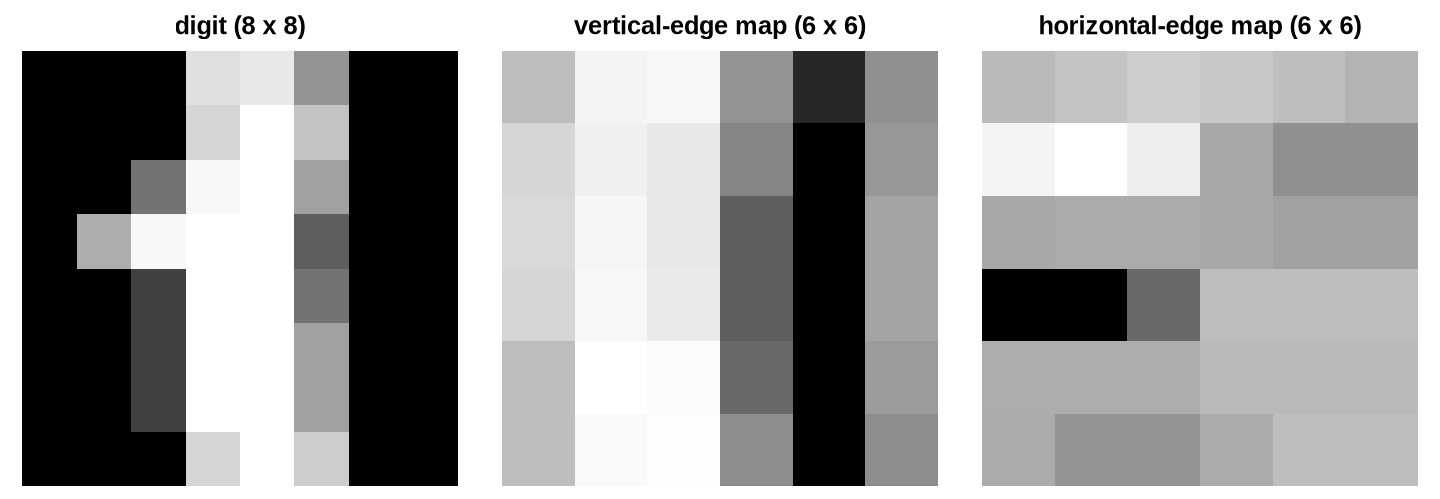
Example 2 (Vertical and horizontal edges in a handwritten 1) Apply \(K_v\) from Exercise 10 and its transpose \(K_h = \tp{K_v}\) to the second digit, which is a handwritten \(1\). \(K_h\) subtracts the row above and adds the row below, so it responds to horizontal edges. Figure 1 shows the grid and both feature maps.
The vertical-edge map has the largest magnitudes, up to 48, along the two long sides of the stroke. The horizontal-edge map is smaller, at most 27 in magnitude, since a straight vertical stroke has few horizontal edges. Each map is \(6 \times 6\).
Show code
show_grid<-function(M, main){# image() draws row 1 at the bottom, so flip the rows to show the grid as printed.image(t(M[rev(seq_len(nrow(M))), ]), col =gray.colors(64, start =0, end =1), axes =FALSE, main =main, asp =1)}op<-par(mfrow =c(1, 3), mar =c(0.5, 0.5, 2, 0.5))show_grid(img_r, "digit (8 x 8)")show_grid(Z_v_r, "vertical-edge map (6 x 6)")show_grid(Z_h_r, "horizontal-edge map (6 x 6)")par(op)
Figure 1: The second digit of the test data (a handwritten 1) and its feature maps under the vertical-edge filter and the horizontal-edge filter. Light squares are large positive sums, dark squares large negative sums.
ExrExercise 15 (Convolution or cross-correlation?)
Exercise 15 (Convolution or cross-correlation?) In signal processing, the convolution of \(X\) with \(K\) is
in which the filter is read backwards: as \(u\) grows, the row of \(X\) shrinks. Equation 1 reads it forwards, and signal processing calls that cross-correlation.
How do the two differ, when both are applied to the same \(X\) and \(K\)?
Solution 15. Substituting \(u' = k + 1 - u\) and \(v' = k + 1 - v\) turns the backwards sum into \(\sum_{u',v'} K_{k+1-u',\,k+1-v'}\, X_{i+u'-1,\,j+v'-1}\), which is Equation 1 applied to the filter flipped top to bottom and left to right. So signal-processing convolution is cross-correlation with a flipped filter.
ExrExercise 16 (Convolution or cross-correlation? (part 2))
Exercise 16 (Convolution or cross-correlation? (part 2)) Use the setup of Exercise 15.
Does the difference matter when \(K\) is learned from data?
Solution 16. When \(K\) is learned, the flip changes nothing. Whatever filtertraining finds under one convention, the flipped filter computes the same feature map under the other, so the two conventions represent the same set of layers and reach the same predictions. Deeplearning libraries compute Equation 1 and call it convolution. These notes do the same, and write cross-correlation when the distinction matters [1, Ch. 9].
ExrExercise 17 (Convolution or cross-correlation? (part 3))
Exercise 17 (Convolution or cross-correlation? (part 3)) Use the setup of Exercise 15.
Check your answer to Exercise 15 on the second digit with \(K_v\).
def true_conv2d(X, K):"""The backwards definition: row i-u+k of X is paired with row u of K.""" k = K.shape[0] Z = np.zeros((X.shape[0] - k +1, X.shape[1] - k +1))for i inrange(Z.shape[0]):for j inrange(Z.shape[1]): Z[i, j] =sum(K[u, v] * X[i + k -1- u, j + k -1- v]for u inrange(k) for v inrange(k))return Zprint(np.allclose(true_conv2d(img_py, K_v), corr2d(img_py, K_v[::-1, ::-1])))
true_conv2d<-function(X, K){# The backwards definition: row i-u+k of X is paired with row u of K.k<-nrow(K)Z<-matrix(0, nrow(X)-k+1, ncol(X)-k+1)for(iinseq_len(nrow(Z))){for(jinseq_len(ncol(Z))){for(uinseq_len(k)){for(vinseq_len(k)){Z[i, j]<-Z[i, j]+K[u, v]*X[i+k-u, j+k-v]}}}}Z}flip_k<-function(K)K[rev(seq_len(nrow(K))), rev(seq_len(ncol(K)))]isTRUE(all.equal(true_conv2d(img_r, K_v_r), corr2d(img_r, flip_k(K_v_r))))
The first check is TRUE: the backwards sum equals cross-correlation with the flipped filter. The second is FALSE: with the filter unflipped the two disagree, here by a sign, since \(K_v\) flipped is \(-K_v\).
VideosWatch
Video 1: Starmer explains convolutional networks for image classification [7].
3 Stride and padding
ExrExercise 18 (Changing the size of the feature map)
Exercise 18 (Changing the size of the feature map) In Solution 14, an \(8 \times 8\) image gave a \(6 \times 6\)feature map.
How could the filter visit fewer positions, to get a smaller feature map?
Solution 18. Move the filter more than one pixel between positions. Stepping two pixels at a time visits about a quarter of the positions of a one-pixel step.
ExrExercise 19 (Changing the size of the feature map (part 2))
Exercise 19 (Changing the size of the feature map (part 2)) Use the setup of Exercise 18.
How could a feature map keep the image’s size, \(8 \times 8\), with a \(3 \times 3\)filter?
Solution 19. Add a border of zeros around the image before sliding the filter. A \(3 \times 3\) filter then fits at the corner pixels too, with the border covering its overhang.
Definition 6 (Stride) The stride\(s\) of a convolution is the number of pixels the filter moves between neighbouring positions, along the rows and the columns [6]. The convolution in Equation 1 has stride \(s = 1\). With stride \(s\), the filter’s top-left corner visits rows \(1, 1+s, 1+2s, \dots\) and columns \(1, 1+s, 1+2s, \dots\).
Definition 7 (Padding)Padding with \(p\) adds \(p\) rows of zeros above and below the image, and \(p\) columns of zeros to its left and right, before the filter slides over it [6]. The padded image is \((H + 2p) \times (W + 2p)\). Convolution with no padding (\(p=0\)) is called “valid” in software; with stride \(1\) and \(p = (k-1)/2\) for odd \(k\) the feature map is as large as the image, and the software calls it “same”.
The feature map is \(8 \times 8\), the same size as the image. Its interior \(6 \times 6\) block equals the unpadded map, and the added outer ring covers the filter positions that overhang the image.
Solution 21. In Exercise 21, the filter’s first position starts at pixel \(1\), and its last at a pixel \(q\) with \(q + k - 1 \le n + 2p\). Positions are \(1, 1+s, \dots, 1+ms\) for the largest integer \(m\) with \(1 + ms \le n + 2p - k + 1\), so \(m = \floor{(n + 2p - k)/s}\) and the number of positions is \(m + 1\).
ExrExercise 22 (The size of the feature map (part 3))
Exercise 22 (The size of the feature map (part 3)) Use the setup of Exercise 20.
Evaluate your formula for \(n = 8\), \(k = 3\) with \((p, s) = (0, 1)\), \((1, 1)\) and \((0, 2)\), and compare with Example 3 and Example 4.
Solution 22. \((0,1)\) gives \(\floor{5/1} + 1 = 6\), \((1,1)\) gives \(\floor{7/1} + 1 = 8\), and \((0,2)\) gives \(\floor{5/2} + 1 = 3\). These are the sizes of the maps in Solution 13, Example 4 and Example 3.
Theorem 1 (Output size of a convolution) Convolving an \(n \times n\) image with a \(k \times k\) filter, padding \(p\) and stride \(s\) gives a feature map that is \(n_{\text{out}} \times n_{\text{out}}\), with
ExmExample 5 (Checking the formula against the code)
Example 5 (Checking the formula against the code) Compare Equation 2 with the shape of corr2d output on the \(8 \times 8\) digit, for filter sizes \(k = 2, 3, 5\), paddings \(0\) to \(2\) and strides \(1\) to \(3\).
import itertoolsout_size =lambda n, k, p, s: (n +2* p - k) // s +1cases_py =list(itertools.product([2, 3, 5], [0, 1, 2], [1, 2, 3]))ok_py = [corr2d(img_py, np.ones((k, k)), stride=s, pad=p).shape == (out_size(8, k, p, s),) *2for k, p, s in cases_py]print(len(ok_py), all(ok_py))
27 True
out_size_r<-function(n, k, p, s)(n+2*p-k)%/%s+1cases_r<-expand.grid(k =c(2, 3, 5), p =0:2, s =1:3)ok_r<-apply(cases_r, 1, function(case){Z<-corr2d(img_r, matrix(1, case[["k"]], case[["k"]]), stride =case[["s"]], pad =case[["p"]])all(dim(Z)==out_size_r(8, case[["k"]], case[["p"]], case[["s"]]))})c(length(ok_r), all(ok_r))
[1] 27 1
The formula gives the shape of the output in all 27 combinations. The formula can also give a size of zero or less, when the filter is larger than the padded image, and then no feature map exists.
A convolutional layer is a fully connected layer with most of its weights fixed at zero and the rest tied together. The next exercise builds that layer explicitly.
ExrExercise 23 (A convolution is a matrix product on the flattened image)
Exercise 23 (A convolution is a matrix product on the flattened image) Flatten the \(8 \times 8\) image into \(\vx \in \mathbb{R}^{64}\) (Definition 1), and flatten the \(6 \times 6\)feature map of Solution 14 the same way. Then the feature map is a matrix \(M\) times \(\vx\).
Solution 24. Row \((i,j)\) is row \(6(i-1) + j\) of \(M\). It reads only the nine pixels of the patch with top-left corner \((i,j)\). Pixel \((i+u-1,\, j+v-1)\) is entry \(8(i+u-2) + j + v - 1\) of \(\vx\), and its weight is \(K_{uv}\). The other \(55\) entries of the row are zero.
ExrExercise 25 (A convolution is a matrix product on the flattened image (part 3))
Exercise 25 (A convolution is a matrix product on the flattened image (part 3)) Use the setup of Exercise 23.
Build \(M\) for \(K_v\) and check that \(M\vx\) is the flattened feature map.
M_r<-matrix(0, 36, 64)used_r<-matrix(FALSE, 36, 64)# entries that hold a filter weightfor(iin1:6){for(jin1:6){for(uin1:3){for(vin1:3){M_r[6*(i-1)+j, 8*(i+u-2)+j+v-1]<-K_v_r[u, v]used_r[6*(i-1)+j, 8*(i+u-2)+j+v-1]<-TRUE}}}}dim(M_r)
The check returns TRUE: row \((i,j)\) of \(M\vx\) is entry \((i,j)\) of the feature map, flattened row by row. Of the 2304 entries of \(M\), 324 hold a filter weight, and those take only 3 distinct values, because \(K_v\) has zeros and repeated entries.
Definition 8 (Parameter sharing (weight sharing, weight tying)) A layer has parameter sharing when one parameter is used at many positions. In a convolutional layer, every output position uses the same filter \(K\) and bias \(b\), and each output reads only the \(k \times k\) patch under the filter, its receptive field[6]. Compared with a fully connected layer on the flattened input, the weight matrix \(M\) of Solution 25 is sparse, and its nonzero entries are tied together. Parameter sharing is also called weight sharing or weight tying.
Example 6 (Counting parameters for the digits) Count the parameters of three layers that read an \(8 \times 8\) image. The first is fully connected with \(36\) units, one for each entry of the \(6 \times 6\) feature map. The second is a convolutional layer with one \(3 \times 3\) filter. The third is a convolutional layer with \(4\) filters.
p_in =8*8fc_36 = (p_in +1) *36# a weight per pixel and a bias, for each unitconv_1 =3*3+1# nine weights and a biasconv_4 =4* (3*3+1)fc_144 = (p_in +1) * (4*36) # a fully connected layer with 4 maps' worth of unitsprint(fc_36, conv_1, conv_4, fc_144)
2340 10 40 9360
p_in_r<-8*8fc_36_r<-(p_in_r+1)*36# a weight per pixel and a bias, for each unitconv_1_r<-3*3+1# nine weights and a biasconv_4_r<-4*(3*3+1)fc_144_r<-(p_in_r+1)*(4*36)# a fully connected layer with 4 maps' worth of unitsc(fc_36_r, conv_1_r, conv_4_r, fc_144_r)
[1] 2340 10 40 9360
A fully connected layer producing one map’s worth of outputs has 2340 parameters; the convolutional layer has 10. With \(4\) feature maps, the counts are 9360 and 40. The convolutional count does not depend on the image size at all: the same \(3 \times 3\) filter on a \(32 \times 32\) image still has 10 parameters, while the fully connected layer’s count grows with the product of the input and output sizes.
Exercise 26 (Shrinking a feature map) Keep the positive part of the \(6 \times 6\) vertical-edge map of Solution 14, setting negative entries to \(0\). Then split it into non-overlapping \(2 \times 2\) blocks and replace each block with its largest entry.
Exercise 28 (Shrinking a feature map (part 3)) Use the setup of Exercise 26.
Shift the digit one pixel to the right and repeat. Is the \(3 \times 3\) result more similar to its unshifted version than the \(6 \times 6\) map is to its unshifted version? Measure similarity by the correlation between the two maps.
max_pool<-function(Z, size=2){out<-matrix(0, nrow(Z)/size, ncol(Z)/size)for(iinseq_len(nrow(out))){for(jinseq_len(ncol(out))){out[i, j]<-max(Z[(i-1)*size+1:size, (j-1)*size+1:size])}}out}relu_map_r<-pmax(Z_v_r, 0)shifted_r<-cbind(0, img_r[, -8])# one pixel right; the last column is emptyrelu_map_sh_r<-pmax(corr2d(shifted_r, K_v_r), 0)max_pool(relu_map_r)
The correlation between the two maps is 0.34 before combining blocks and 0.65 after. A shift of one pixel moves the large responses to a neighbouring column of the map, and the block maximum can keep its value when a response moves within its block.
Definition 9 (Pooling (subsampling)) A pooling layer replaces each \(\poolsize \times \poolsize\) block of a feature map by one number, usually moving the block by \(\poolsize\) pixels (stride \(\poolsize\)), so that blocks do not overlap [6]. Max pooling takes the largest entry of the block, and average pooling takes their mean. Pooling has no parameters. It is also called subsampling or downsampling, though downsampling covers other operations too. A \(\poolsize \times \poolsize\) pooling layer turns an \(\imgheight \times \imgwidth\) map into an \((\imgheight/\poolsize) \times (\imgwidth/\poolsize)\) map when \(\poolsize\) divides \(\imgheight\) and \(\imgwidth\).
Example 7 (Max and average pooling on one map) Pool the \(6 \times 6\) positive part of the vertical-edge map with \(\poolsize = 2\), by maximum and by mean.
Both outputs are \(3 \times 3\). The maximum keeps each block’s strongest response, up to 48, and the mean spreads that response over the block, so it is never larger.
A layer usually applies several filters to the same input, and a later layer reads all of their feature maps together.
Definition 10 (Channel) A channel is one \(H \times W\) grid in an array of shape \(H \times W \times C\) with \(C\) channels. A colour image has \(C = 3\) channels (red, green, blue), a greyscale image such as a digit has \(C = 1\), and the feature maps produced by \(F\) filters form an array with \(C = F\) channels. A filter that reads \(C\) input channels has shape \(k \times k \times C\): it multiplies and adds over the \(k \times k\) patch in every channel at once, so it produces one feature map. A convolutional layer with \(F\) such filters has \(F(k^2 C + 1)\) parameters, counting one bias per filter. The number of channels is sometimes called the depth of the array, which differs from the depth of a network.
ExmExample 8 (Channels through two convolutional layers)
Example 8 (Channels through two convolutional layers) The first layer of the digit network has \(F_1 = 4\) filters of size \(3 \times 3\) on the single channel of the digit. A second convolutional layer with \(F_2 = 6\) filters of size \(2 \times 2\) reads the \(4\) channels the first layer produces. Count each layer’s parameters.
The first layer has 40 parameters and the second 102. Each of the second layer’s filters has \(2 \times 2 \times 4 = 16\) weights, since it reads all four channels, and the layer has six of them.
6 A small convolutional network
ExrExercise 29 (A small network for the digits, end to end)
Exercise 29 (A small network for the digits, end to end) Design a network for the \(8 \times 8\) digits with these layers:
a convolutional layer with \(4\) filters of size \(3 \times 3\), stride \(1\), no padding, followed by ReLU;
\(2 \times 2\) max pooling;
flattening;
a fully connected layer with \(10\) outputs, one for each digit, followed by softmax.
Solution 29. Layer by layer, Equation 2 gives the shapes: the convolution maps \(8 \times 8 \times 1\) to \(6 \times 6 \times 4\), the pooling gives \(3 \times 3 \times 4\), flattening gives a vector of \(36\) numbers, and the output layer maps it to \(10\).
ExrExercise 30 (A small network for the digits, end to end (part 2))
Exercise 30 (A small network for the digits, end to end (part 2)) Use the setup of Exercise 29.
Solution 30. The convolution has \(4(9 + 1) = 40\)parameters, the pooling and the flattening have none, and the output layer has \(10 \times (36 + 1) = 370\) parameters.
ExrExercise 31 (A small network for the digits, end to end (part 3))
Exercise 31 (A small network for the digits, end to end (part 3)) Use the setup of Exercise 29.
Pass the second digit through the network with random weights to check the shapes.
The shapes match: \(8 \times 8\), then \(6 \times 6 \times 4\), \(3 \times 3 \times 4\), \(36\) and \(10\), and the ten outputs sum to 1. The weights are random, so the ten probabilities carry no information about the digit; fitting the weights is a job for gradient descent and backpropagation.
ExrExercise 32 (A small network for the digits, end to end (part 4))
Exercise 32 (A small network for the digits, end to end (part 4)) Use the setup of Exercise 29.
Remark 1 (Training a convolutional network). Backpropagation works on a convolutional network as on any composition of differentiable layers, with two additions. A filter weight \(K_{uv}\) is used at every output position, so its gradient is the sum over positions of the gradient each use contributes, as the chain rule gives for a variable that appears many times. Max pooling passes the gradient only to the entry that was largest in its block, since the other entries did not affect the output. The same sum over uses returns for recurrent layers, where a weight is used at every time step.
LeCun et al. [8] used this pipeline of convolution, pooling and a final classifier to read handwritten digits.
7 Recurrent layers
An image has a fixed size, and its neighbours lie in two directions. A series has an order and no fixed length.
Exercise 33 (A series as input) The Smarket data hold the daily returns (percent change) of the S&P 500 index on 1250 trading days from 2001 to 2005 [5, Ch. 4]. The rows are in time order, and Lag1 is the previous day’s return.
Check that the first \(30\) rows are \(30\) consecutive trading days, by comparing each Lag1 with the previous row’s Today.
Exercise 34 (A series as input (part 2)) Use the setup of Exercise 33.
A fully connected layer taking these \(30\) returns as its \(30\) inputs would be tied to the length \(30\). Name two other things it handles badly when the inputs are a time series.
Solution 34. A fully connected layer gives each day its own weights, so it must learn the same pattern again for every position in the window. It also cannot take a series of \(31\) days when it was built for \(30\), and, as in Solution 8, it is blind to which days are adjacent.
Exercise 35 (Carrying a memory along a series) Standardize the daily returns by dividing by their standard deviation in the full data, and call the first three standardized returns \(z_1, z_2, z_3\). Keep a state of two numbers \(\vhidval_t\), starting from \(\vhidval_0 = \vzero\), and update it each day by
Solution 36. The state \(\vhidval_3\) depends on all three returns: \(z_3\) enters directly, \(z_2\) enters through \(\vhidval_2\), and \(z_1\) through \(\vhidval_1\) and then \(\vhidval_2\). The same \(W_h\) and \(\vw_x\) are used at all three steps, and the state keeps a length of two however long the series.
Definition 11 (Recurrent layer) A recurrent layer reads a sequence \(\vx_1, \dots, \vx_T\) with \(\vx_t \in \mathbb{R}^{\ninputvars}\) and keeps a state \(\vhidval_t \in \mathbb{R}^{H}\), updated at each step by
with \(W_x \in \mathbb{R}^{H \times \ninputvars}\), \(W_h \in \mathbb{R}^{H \times H}\), a bias\(\vecf{b} \in \mathbb{R}^{H}\) and an activation \(f\) applied coordinate by coordinate. The same \(W_x\), \(W_h\) and \(\vecf{b}\) are used at every step. Predictions are read from the states, such as \(g(U\vhidval_t)\) at each step or only at \(t = T\). The layer in Equation 4 is the simple or Elman recurrent layer [9].
Definition 12 (Hidden state (memory)) The hidden state\(\vhidval_t \in \reals^{H}\) of a recurrent layer (Definition 11) is the state it keeps and updates at each step by Equation 4. The state \(\vhidval_t\) is also called the memory.
Definition 13 (Recurrent neural network (RNN)) A network built from recurrent layers (Definition 11) is a recurrent neural network (RNN) [10].
ExmExample 9 (The hidden state over thirty trading days)
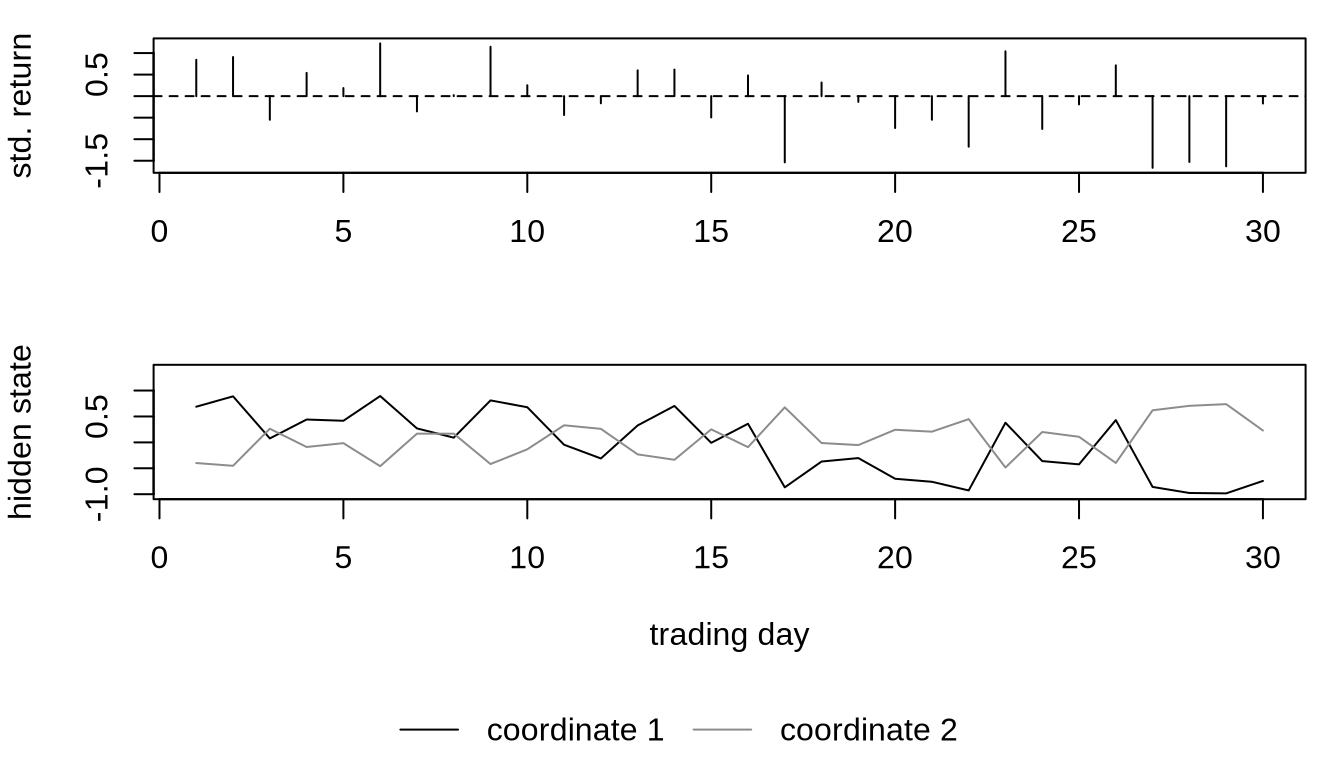
Example 9 (The hidden state over thirty trading days) Run Equation 3 over the first \(30\) standardized returns, and again over only the first \(10\). Figure 2 plots the thirty states.
The same layer takes a series of \(10\) days and one of \(30\) days, with 6 weights in both cases. The state after day \(10\) is the same in the two runs, since later days cannot change it.
Show code
# The outer margin leaves room under the lower panel for its legend.op<-par(mfrow =c(2, 1), mar =c(4, 4, 1, 1), oma =c(3, 0, 0, 0))plot(1:30, z_r[1:30], type ="h", xlab ="", ylab ="std. return")abline(h =0, lty =2)matplot(1:30, H30_r, type ="l", lty =1, col =c("black", "grey55"), ylim =c(-1, 1.4), xlab ="trading day", ylab ="hidden state")# An empty plot over the whole device places the legend in the outer margin.par(fig =c(0, 1, 0, 1), oma =c(0, 0, 0, 0), mar =c(0, 0, 0, 0), new =TRUE)plot.new()legend("bottom", legend =c("coordinate 1", "coordinate 2"), lty =1, col =c("black", "grey55"), bty ="n", horiz =TRUE)par(op)
Figure 2: The standardized daily returns of the first 30 trading days of the Smarket data (top), and the two coordinates of the hidden state of the toy recurrent layer (bottom).
Solution 37. \(W_x\) has \(H\ninputvars\) entries, \(W_h\) has \(H^2\) and \(\vecf{b}\) has \(H\), so the layer has \(H(\ninputvars + H + 1)\)parameters.
ExrExercise 38 (Parameters of a recurrent layer (part 2))
Exercise 38 (Parameters of a recurrent layer (part 2)) Use the setup of Exercise 37.
Does the count change with the length \(T\) of the series?
Solution 39. \(H(T\ninputvars + 1)\), which grows with \(T\).
DefDefinition 14 (Unrolling (unfolding through time))
Definition 14 (Unrolling (unfolding through time))Unrolling a recurrent layer over \(T\) steps writes it as a feedforward network with \(T\) copies of the same layer: copy \(t\) takes \(\vx_t\) and the output \(\vhidval_{t-1}\) of copy \(t-1\), and returns \(\vhidval_t\). All copies share their parameters (Definition 8). Unrolling is also called unfolding through time. The unrolled network has depth\(T\), where \(T\) is the length of the series.
Example 10 (Unrolled over thirty days) A toy recurrent layer has \(\ninputvars = 1\)input and \(H = 2\) units. Count the weights of its unrolled network over \(T = 30\) days, with and without sharing, and for a fully connected layer on the \(30\) returns.
With sharing, the unrolled network has 8 parameters, as the layer does. Thirty independent copies would have 240. A fully connected layer with two units on all thirty returns has 62, and it fits a series of exactly thirty days only.
VideosWatch
Video 2: Starmer explains recurrent neural networks [11].
8 Backpropagation through time
Reuse of the weights across steps is also what makes the gradient hard.
ExrExercise 40 (How the state depends on an earlier state)
Exercise 40 (How the state depends on an earlier state) Consider Equation 4 with \(f = \tanh\) and write \(\va_t = W_x \vx_t + W_h \vhidval_{t-1} + \vecf{b}\). The Jacobian \(\derivf{\vhidval_t}{\vhidval_{t-1}}\) is the \(H \times H\) matrix whose entry \((i,j)\) is \(\partial \hidvalof{t,i} / \partial \hidvalof{t-1,j}\).
Solution 40. The derivative of \(\tanh\) is \(1 - \tanh^2\), so \(\vhidval_t = \tanh(\va_t)\) has the diagonal Jacobian \(\derivf{\vhidval_t}{\va_t} = D_t\), where \(D_t = \diagf{1 - \hidvalof{t,1}^2, \dots, 1 - \hidvalof{t,H}^2}\). Also \(\derivf{\va_t}{\vhidval_{t-1}} = W_h\). The chain rule multiplies the two:
Solution 41. Because \(\vhidval_T\) depends on \(\vhidval_k\) through \(\vhidval_{T-1}, \dots, \vhidval_{k+1}\), the chain rule multiplies one factor for each step:
It is a product of \(T - k\) matrices, all built from the one matrix \(W_h\).
LemTheorem 2 (Jacobian of the state of a tanh recurrent layer)
Theorem 2 (Jacobian of the state of a tanh recurrent layer) For a recurrent layer with \(f = \tanh\) and \(\va_t = W_x \vx_t + W_h \vh_{t-1} + \vecf{b}\), let \(D_t = \diagf{1 - h_{t,1}^2, \dots, 1 - h_{t,H}^2}\). Then
ExrExercise 42 (Why the gradient vanishes or explodes)
Exercise 42 (Why the gradient vanishes or explodes) Let \(\norm{\cdot}\) denote the spectral norm of a matrix, its largest singular value. Use Theorem 2.
Bound \(\norm{D_t}\), then bound \(\norm{\derivf{\vhidval_T}{\vhidval_k}}\) in terms of \(\norm{W_h}\).
Solution 42. \(D_t\) is diagonal with entries \(1 - \hidvalof{t,i}^2 \in (0, 1]\), so \(\norm{D_t} \le 1\). The spectral norm of a product is at most the product of the norms, so
Solution 43. When \(\norm{W_h} < 1\), the bound \(\norm{W_h}^{T-k}\) shrinks geometrically in \(T - k\). A change in \(\vhidval_k\) then has an exponentially small effect on \(\vhidval_T\), and so a loss that depends on \(\vhidval_T\) sends exponentially small gradient to the early steps. The gradient vanishes.
ExrExercise 44 (Why the gradient vanishes or explodes (part 3))
Exercise 44 (Why the gradient vanishes or explodes (part 3)) Use the setup of Exercise 42.
If the activation were the identity, so that every \(D_t\) were the identity matrix, what would \(\derivf{\vhidval_T}{\vhidval_k}\) be?
Solution 44. With the identity activation, \(\derivf{\vhidval_T}{\vhidval_k} = W_h^{T-k}\).
ExrExercise 45 (Why the gradient vanishes or explodes (part 4))
Exercise 45 (Why the gradient vanishes or explodes (part 4)) Use the setup of Exercise 42.
With the identity activation, what happens to the norm of \(\derivf{\vhidval_T}{\vhidval_k}\) if \(W_h\) has an eigenvalue of absolute value greater than \(1\)?
Solution 45. If \(W_h\) has an eigenvalue \(\lambda\) with \(\abs{\lambda} > 1\) and eigenvector \(\vv\), then \(W_h^{T-k}\vv = \lambda^{T-k}\vv\), which grows geometrically, so \(\norm{W_h^{T-k}} \ge \abs{\lambda}^{T-k}\) and the gradient can explode. With \(\tanh\), the factors \(D_t\) shrink the product, and the bound of Solution 42 does not rule out growth: it only limits it.
whatever the inputs [12], [13]. If \(\norm{W_h} < 1\), the gradient of a loss at step \(T\) with respect to earlier states vanishes exponentially in \(T - k\).
ExmExample 11 (Gradient norms over thirty trading days)
Example 11 (Gradient norms over thirty trading days) Take four hidden units, with \(W_h = \rho Q\) for a rotation matrix \(Q\), so that \(\norm{W_h} = \rho\) exactly. Drive the layer with the \(30\) standardized returns, with input weights \((0.5, -0.3, 0.4, 0.2)\) chosen for illustration. Compute \(\norm{\derivf{\vhidval_m}{\vhidval_0}}\) for \(m = 1, 5, 10, 20, 30\) and \(\rho = 0.5, 0.9, 1, 1.5\), and compare it with the bound \(\rho^m\).
In each table, the rows are \(\rho\) and the columns are the lags. Every norm is below its bound: TRUE. For \(\rho = 0.5\) the norm falls to 1.1e-10 by lag \(30\). Even for \(\rho = 1\) it falls, to 1.2e-02, because the factors \(D_t\) shrink the product. For \(\rho = 1.5\) the norm is 11 at lag \(30\), above \(1\) but far below the bound 1.9e+05 that the identity activation attains.
ExrExercise 46 (The gradient for the shared weights)
Exercise 46 (The gradient for the shared weights) Suppose the loss\(\loss\) depends on the layer only through the last state \(\vhidval_T\). Let \(\vg_t = \derivf{\loss}{\va_t}\), with \(\va_t\) as in Exercise 40.
Express \(\vg_t\) in terms of \(\derivf{\loss}{\vhidval_t}\), and \(\derivf{\loss}{\vhidval_{t-1}}\) in terms of \(\vg_t\).
Solution 46. Since \(\vhidval_t = \tanh(\va_t)\), the chain rule gives \(\vg_t = D_t\, \derivf{\loss}{\vhidval_t}\). Since \(\va_t\) depends on \(\vhidval_{t-1}\) through \(W_h \vhidval_{t-1}\), it gives \(\derivf{\loss}{\vhidval_{t-1}} = \tp{W_h}\, \vg_t\). Starting from \(\derivf{\loss}{\vhidval_T}\), which the loss supplies, these two rules produce \(\vg_T, \vg_{T-1}, \dots, \vg_1\) in turn.
ExrExercise 47 (The gradient for the shared weights (part 2))
Exercise 47 (The gradient for the shared weights (part 2)) Use the setup of Exercise 46.
The matrix \(W_h\) is used at every step. Find \(\derivf{\loss}{W_h}\).
LemTheorem 4 (The backward recursion and the shared-weight gradient)
Theorem 4 (The backward recursion and the shared-weight gradient) Suppose the loss \(L\) depends on a tanh recurrent layer only through the last state \(\vh_T\), and let \(\vg_t = \derivf{L}{\va_t}\). Then
ExmExample 12 (Checking the backward recursion on a small layer)
Example 12 (Checking the backward recursion on a small layer) Take a tanh recurrent layer with \(H = 2\) units and \(T = 3\) steps, scalar inputs, and the loss \(L = \sum_i h_{T,i}\). Compute \(\derivf{L}{W_h}\) by the recursion of Theorem 4, and compare it with a finite difference of the loss:
Definition 15 (Backpropagation through time)Backpropagation through time (BPTT) is backpropagation on the unrolled network (Definition 14) [14]. It runs the forward pass over all \(T\) steps, storing the states, then passes \(\derivf{L}{\vhidval_t}\) backwards from \(t = T\) to \(t = 1\) by the rules of Theorem 4, and adds each step’s contribution to the gradient of the shared weights. The cost grows linearly in \(T\) in both time and memory. When the loss also depends on the states at earlier steps, the direct term \(\derivf{L_t}{\vhidval_t}\) is added to \(\derivf{L}{\vhidval_t}\) at each step.
ExmExample 13 (Checking BPTT against finite differences)
Example 13 (Checking BPTT against finite differences) Take the toy layer of Equation 3 on the first \(10\) days, and the loss \(L = \hidvalof{10,1}\), the first coordinate of the last state. Compute \(\derivf{L}{W_h}\) by BPTT, and compare it with a central finite difference in each of the four entries of \(W_h\).
The two methods agree to 8e-11. BPTT needed one backward pass, whereas the finite differences needed two extra forward passes for each of the four entries of \(W_h\).
Remark 2 (Repairs for exploding gradients). When the gradient explodes, gradient clipping rescales it before the update. Clipping does not help a vanishing gradient, which is too small to rescale usefully. Initializing \(W_h\) near an orthogonal matrix keeps \(\norm{W_h}\) near \(1\) at the start of training, as the initializations of the backpropagation chapter do for fully connected layers. The more lasting fix changed the architecture, as the next section describes.
9 Gates
ExrExercise 48 (A path for memory that does not decay)
Exercise 48 (A path for memory that does not decay) In Equation 4, the old state \(\vhidval_{t-1}\) passes through \(W_h\) and \(\tanh\) before it reaches \(\vhidval_t\). Design a second vector \(\vecf{c}_t \in \mathbb{R}^H\), updated from \(\vecf{c}_{t-1}\) and a new candidate \(\vecf{u}_t\), so that the network can choose, coordinate by coordinate, to keep an old value unchanged, erase it, or overwrite it.
Solution 48. Multiply the old value by a number between \(0\) and \(1\) that the network computes at each step, and add a new contribution scaled the same way:
where \(\odot\) multiplies coordinate by coordinate, and \(\vecf{f}_t\) and \(\vecf{i}_t\) have all entries in \((0,1)\). A coordinate of \(\vecf{f}_t\) near \(1\) keeps the old value and near \(0\) erases it, and a coordinate of \(\vecf{i}_t\) near \(1\) admits the new candidate and near \(0\) ignores it.
ExrExercise 49 (A path for memory that does not decay (part 2))
Exercise 49 (A path for memory that does not decay (part 2)) Use the setup of Exercise 48.
What is \(\derivf{\vecf{c}_t}{\vecf{c}_{t-1}}\) in your design?
Solution 49. Along this path, \(\derivf{\vecf{c}_t}{\vecf{c}_{t-1}} = \diag(\vecf{f}_t)\), with no weight matrix and no \(\tanh\) in the way. If the network sets \(\vecf{f}_t\) close to \(1\), the gradient passes through many steps almost unchanged.
Definition 17 (Long short-term memory (LSTM)) A long short-term memory (LSTM) layer keeps a cell state \(\vecf{c}_t\) and a hidden state \(\vhidval_t\), both in \(\mathbb{R}^H\)[15]. Three gates (Definition 16) control the cell state:
The cell state carries memory, and the output gate decides how much of it the hidden state shows. The layer has four weight blocks of the same shape as a simple recurrent layer’s, so \(4H(\ninputvars + H + 1)\)parameters. The original LSTM [16] had no forget gate; it was added later [17], and modern libraries include it.
ExmExample 14 (How much of the cell state survives thirty steps)
Example 14 (How much of the cell state survives thirty steps) Along the cell-state path, the derivative of \(\vecf{c}_{30}\) with respect to \(\vecf{c}_0\) is the product of the forget gates. Compute it for a coordinate whose forget gate is held at \(0.5\), \(0.9\) and \(0.99\) at every step.
A forget gate of \(0.5\) leaves 9.3e-10 of the signal, which is a vanished gradient. A gate of \(0.99\) leaves 0.74. The network learns its gates, so it can hold them near \(1\) for a coordinate that must remember. This is the direct cell-state path only: the gates also depend on \(\vhidval_{t-1}\), which adds paths through the recurrent weights.
Remark 3 (The gated recurrent unit). The gated recurrent unit (GRU) [18] merges the cell and hidden states and uses two gates instead of three. An update gate \(\vecf{z}_t\) and a reset gate \(\vecf{r}_t\), both computed like \(\vecf{f}_t\) in Equation 5, give
The gate \(\vecf{z}_t\) plays the role of both \(\vecf{f}_t\) and \(\vecf{i}_t\) of the LSTM, tied so that they sum to one. Sources differ on whether \(\vecf{z}_t\) or \(1 - \vecf{z}_t\) multiplies the old state. A GRU has three weight blocks, so \(3H(\ninputvars + H + 1)\)parameters.
10 Where this goes next
Gated recurrent layers read a sequence one step at a time, so step \(t\) cannot start before step \(t-1\) finishes, and information from step \(1\) reaches step \(T\) only through \(T-1\) updates of the state. Attention and Transformers replaces the recurrence: every position reads every other position directly, and all positions are computed at once. Transformers have replaced recurrent networks in most language models, and convolutional layers remain standard for images, audio and other data on a grid.
11 Further reading
Goodfellow et al. [1], Chapter 9 (convolutional networks) and Chapter 10 (sequence modeling)
James et al. [2], Chapter 10, which covers convolutional and recurrent networks; James et al. [5] has the Python version
VideosWatch
Andrew Ng’s lectures for DeepLearning.AI, on convolutional networks, cover: convolution as edge detection [19]; padding [20]; strided convolutions [21]; pooling layers [22]; and why convolutions suit images [23].
G. James, D. Witten, T. Hastie, and R. Tibshirani, An introduction to statistical learning with applications in R, 2nd ed. Springer, 2021. Available: https://www.statlearning.com/
[3]
V. Dumoulin and F. Visin, “A guide to convolution arithmetic for deep learning.” 2016. Available: https://arxiv.org/abs/1603.07285
[4]
E. Alpaydin and C. Kaynak, “Optical recognition of handwritten digits.”UCI Machine Learning Repository, 1998. doi: 10.24432/C50P49.
[5]
G. James, D. Witten, T. Hastie, R. Tibshirani, and J. Taylor, An introduction to statistical learning: With applications in Python. Springer, 2023. doi: 10.1007/978-3-031-38747-0.
J. Starmer, “Neural networks part 8: Image classification with convolutional neural networks (CNNs).” StatQuest, video on YouTube, 2021. Available: https://www.youtube.com/watch?v=HGwBXDKFk9I
[8]
Y. LeCun, L. Bottou, Y. Bengio, and P. Haffner, “Gradient-based learning applied to document recognition,”Proceedings of the IEEE, vol. 86, no. 11, pp. 2278–2324, 1998, doi: 10.1109/5.726791.
[9]
J. L. Elman, “Finding structure in time,”Cognitive Science, vol. 14, no. 2, pp. 179–211, 1990, doi: 10.1207/s15516709cog1402_1.
Y. Bengio, P. Simard, and P. Frasconi, “Learning long-term dependencies with gradient descent is difficult,”IEEE Transactions on Neural Networks, vol. 5, no. 2, pp. 157–166, 1994, doi: 10.1109/72.279181.
[13]
R. Pascanu, T. Mikolov, and Y. Bengio, “On the difficulty of training recurrent neural networks,” in Proceedings of the 30th international conference on machine learning, 2013, pp. 1310–1318. Available: https://arxiv.org/abs/1211.5063
S. Hochreiter and J. Schmidhuber, “Long short-term memory,”Neural Computation, vol. 9, no. 8, pp. 1735–1780, 1997, doi: 10.1162/neco.1997.9.8.1735.
[17]
F. A. Gers, J. Schmidhuber, and F. Cummins, “Learning to forget: Continual prediction with LSTM,”Neural Computation, vol. 12, no. 10, pp. 2451–2471, 2000, doi: 10.1162/089976600300015015.
[18]
K. Cho et al., “Learning phrase representations using RNN encoder–decoder for statistical machine translation,” in Proceedings of the 2014 conference on empirical methods in natural language processing, 2014, pp. 1724–1734.