Neural Networks Lab

Published

Last modified: 2026-11-19

Show code
# The Python chunks on this page import matplotlib, numpy, pandas
# and scikit-learn; reticulate provisions them.
py_packages <- c("matplotlib", "numpy", "pandas", "scikit-learn")
library(reticulate) # nolint: undesirable_function_linter
library(tidymodels) # nolint: undesirable_function_linter
py_require(py_packages)
1 The book’s Chapter 10 lab

This page holds the code lab for the Neural Networks chapter.

To work the lab without the solutions, download a stub with only the exercises:

Each solution shows the code in Python and in R.

Section 10.9.1 of the book [1] is the source of these exercises. The book uses PyTorch and the R package keras for this step. This lab uses scikit-learn [2] in Python and the nnet engine of tidymodels in R, which fit a single hidden layer with no extra framework.

2 Exploring the Hitters data

DatasetDataset 1: The baseball (Hitters) data
Dataset 1: The baseball (Hitters) data

Statistics and salaries of major league baseball players on 322 rows make up the Hitters data [1, Sec. 10.9.1]. The data are in data/hitters.csv, one row per player. The columns this course uses are:

  • Salary: the outcome, the player’s salary in thousands of dollars, missing for some players.
  • CHits: the number of hits during the player’s career.
  • Years: the number of years the player has played in the major leagues.
  • The other numeric columns: batting and fielding counts for the previous season and for the career.
ExrExercise 1 (Lab: players with a missing salary)

Exercise 1 (Lab: players with a missing salary) Use the Hitters data. How many players have a missing Salary?

TipHint

Count the missing values of a column with a pandas method in Python, or with is.na() in R.

Solution 1.

import pandas as pd

hit_eda_py = pd.read_csv("data/hitters.csv")
hit_eda_py_missing = int(hit_eda_py["Salary"].isna().sum())
hit_eda_py_missing
59
hit_eda_r <- readr::read_csv("data/hitters.csv", show_col_types = FALSE)
hit_eda_r_is_missing <- is.na(hit_eda_r$Salary)
hit_eda_r_missing <- sum(hit_eda_r_is_missing)
hit_eda_r_missing
[1] 59

59 of the 322 players, or 18.3%, have no recorded Salary. The next exercises drop them, because the outcome has to be known to fit a model.

ExrExercise 2 (Lab: salary and career hits)

Exercise 2 (Lab: salary and career hits) Use the Hitters data. Among the players with a recorded Salary, what is the sample correlation between Salary and CHits?

TipHint

Drop the rows with a missing value before you compute it, because a missing value makes the result missing in R and is skipped in pandas.

Solution 2. This solution continues Solution 1.

hit_py_known = hit_eda_py.dropna(subset=["Salary"])
hit_eda_py_cor = float(hit_py_known["Salary"].corr(hit_py_known["CHits"]))
round(hit_eda_py_cor, 3)
0.549
hit_r_known <- hit_eda_r |>
  tidyr::drop_na(Salary)
hit_eda_r_cor <- cor(hit_r_known$Salary, hit_r_known$CHits)
round(hit_eda_r_cor, 3)
[1] 0.549

The correlation is 0.55 among the 263 players with a recorded Salary, so players with more career hits tend to earn more.

ExrExercise 3 (Lab: a histogram of salary)

Exercise 3 (Lab: a histogram of salary) Use the Hitters data. Draw a histogram of Salary for the players with a recorded Salary.

TipHint

Draw a histogram of one column, as in the histogram of the year of each car in the primer.

Solution 3. This solution continues Solution 2.

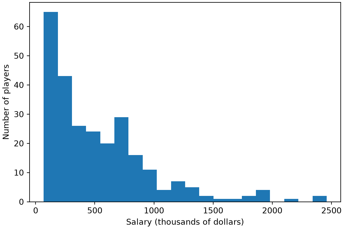
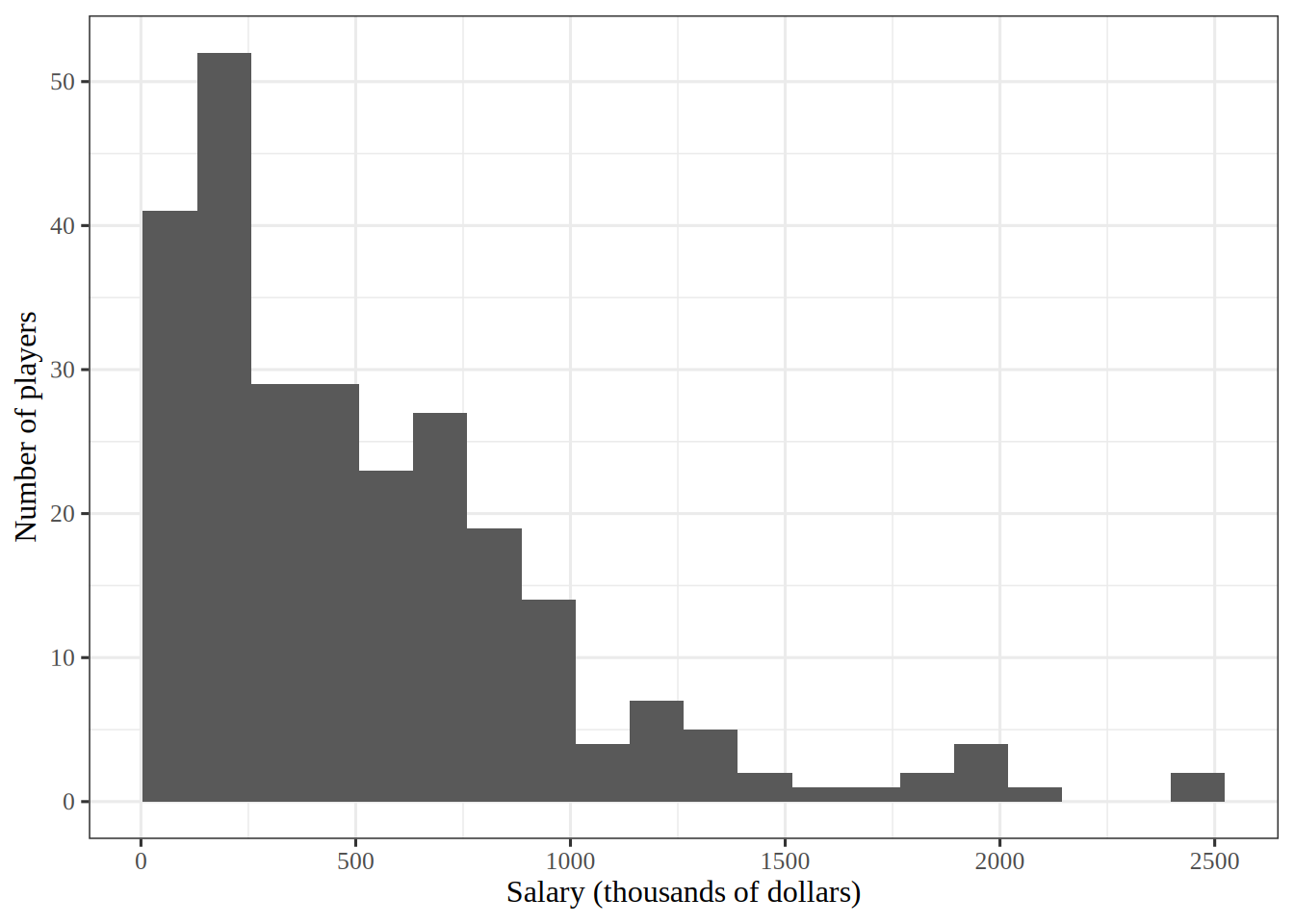
Figure 1: Bars counting the players at each salary, in thousands of dollars.
import matplotlib.pyplot as plt

fig, ax = plt.subplots(figsize=(6, 4), layout="constrained")
ax.hist(hit_py_known["Salary"], bins=20);
ax.set_xlabel("Salary (thousands of dollars)");
ax.set_ylabel("Number of players");
plt.show()

Histogram of baseball player salaries in thousands of dollars. The tallest bars are at the lowest salaries, and the bars shrink steadily toward a long thin tail that reaches the highest salaries.

library(ggplot2) # nolint: undesirable_function_linter

salary_histogram <- hit_r_known |>
  ggplot() +
  aes(Salary) +
  geom_histogram(bins = 20) +
  labs(x = "Salary (thousands of dollars)", y = "Number of players")
salary_histogram

Histogram of baseball player salaries in thousands of dollars. The tallest bars are at the lowest salaries, and the bars shrink steadily toward a long thin tail that reaches the highest salaries.

Show code
hit_eda_r_median <- median(hit_r_known$Salary)
hit_eda_r_mean <- mean(hit_r_known$Salary)
hit_eda_r_per_bin <- nrow(hit_r_known) / 20

I chose 20 bins, which is about 13 players per bar on average. Far fewer bins would hide the long right tail inside a few wide bars, and far more would leave most bars with only a few players, so the outline would look ragged. That is why 20 is a compromise between the two.

Figure 1 shows a strongly right-skewed shape: the sample median is 425 thousand dollars, far below the sample mean of 536 thousand dollars.

ExrExercise 4 (Lab: salary against career hits)

Exercise 4 (Lab: salary against career hits) Use the Hitters data. Draw a scatterplot of Salary against CHits for the players with a recorded Salary.

TipHint

Draw a scatterplot of one column against another, as in the plot of acceleration against horsepower in the primer.

Solution 4. This solution continues Solution 2.

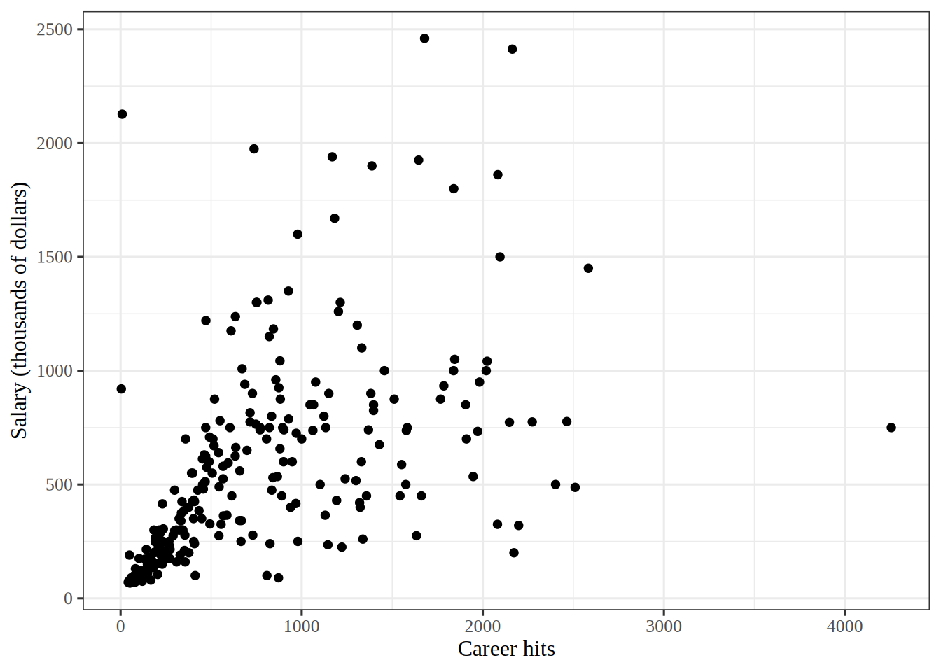
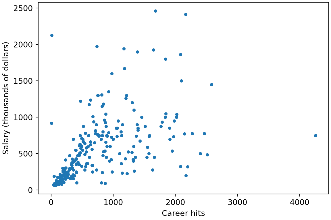
Figure 2: Salary, in thousands of dollars, against career hits, with one dot per player.
import matplotlib.pyplot as plt

fig, ax = plt.subplots(figsize=(6, 4), layout="constrained")
ax.scatter(hit_py_known["CHits"], hit_py_known["Salary"], s=10);
ax.set_xlabel("Career hits");
ax.set_ylabel("Salary (thousands of dollars)");
plt.show()

Scatterplot of baseball player salary in thousands of dollars against career hits. The points rise from the lower left, and the vertical spread widens as career hits grow. Most points sit at low salaries and the high-salary points are sparse.

library(ggplot2) # nolint: undesirable_function_linter

salary_chits_plot <- hit_r_known |>
  ggplot() +
  aes(CHits, Salary) +
  geom_point() +
  labs(x = "Career hits", y = "Salary (thousands of dollars)")
salary_chits_plot

Scatterplot of baseball player salary in thousands of dollars against career hits. The points rise from the lower left, and the vertical spread widens as career hits grow. Most points sit at low salaries and the high-salary points are sparse.

In Figure 2, salary rises with career hits but with a widening spread, so a straight line through the points would describe the players with few career hits better than the players with many.

3 Preparing the data

ExrExercise 5 (Lab: load the Hitters data)

Exercise 5 (Lab: load the Hitters data) Read the Hitters data [1], which record the Salary in thousands of dollars of major league baseball players, and keep the \(16\) numeric predictors of Salary. Drop the players whose Salary is missing.

TipHint

The data frame functions read the file and select columns, and .dropna removes the rows with a missing value. In R, drop_na() does the same.

Solution 5.

import numpy as np
import pandas as pd

hitters = pd.read_csv("data/hitters.csv").dropna(subset=["Salary"])
numeric_x = hitters.drop(columns=["Salary", "League", "Division", "NewLeague"])
numeric_x.shape
(263, 16)
hitters <- readr::read_csv("data/hitters.csv", show_col_types = FALSE)
hitters_num <- hitters |>
  drop_na(Salary) |>
  select(-League, -Division, -NewLeague)
dim(hitters_num)
[1] 263  17

The Hitters data have 322 players, 59 of them with a missing Salary. The 263 players left have 16 numeric predictors.

ExrExercise 6 (Lab: split the Hitters data)

Exercise 6 (Lab: split the Hitters data) Split the players from Exercise 5 at random into a training set with two thirds of them and a test set with the rest.

TipHint

The random number functions draw row positions without repeats, and a selection by position keeps those rows.

Solution 6.

from sklearn.model_selection import train_test_split

split_py = train_test_split(
    numeric_x, hitters["Salary"], test_size=1 / 3, random_state=0
)
x_train, x_test, y_train, y_test = split_py
(len(y_train), len(y_test))
(175, 88)
set.seed(571)
split_r <- initial_split(hitters_num, prop = 2 / 3)
train_r <- training(split_r)
test_r <- testing(split_r)
n_train <- nrow(train_r)
n_test <- nrow(test_r)
split_sizes <- c(n_train, n_test)
split_sizes
[1] 175  88

The training set holds 175 players and the test set 88 in the R run, and 175 and 88 in the Python run. The two runs use different random splits.

ExrExercise 7 (Lab: standardize the Hitters predictors)

Exercise 7 (Lab: standardize the Hitters predictors) Standardize each predictor in the training set and the test set from Exercise 6 with its mean and standard deviation in the training set.

TipHint

Broadcasting subtracts a mean and divides by a standard deviation for every column at once, and both numbers come from the training set alone.

Solution 7.

from sklearn.preprocessing import StandardScaler

scaler = StandardScaler().fit(x_train)
x_train_z = scaler.transform(x_train)
x_test_z = scaler.transform(x_test)
x_train_z.mean(axis=0).round(3)
array([-0., -0.,  0.,  0.,  0.,  0.,  0.,  0., -0., -0., -0., -0.,  0.,
        0., -0., -0.])
train_x <- select(train_r, -Salary)
test_x <- select(test_r, -Salary)
train_center <- colMeans(train_x)
train_sd <- map_dbl(train_x, sd)
train_z <- scale(train_x, center = train_center, scale = train_sd) |>
  as_tibble() |>
  mutate(Salary = train_r$Salary)
test_z <- scale(test_x, center = train_center, scale = train_sd) |>
  as_tibble() |>
  mutate(Salary = test_r$Salary)
train_means_z <- select(train_z, -Salary) |> colMeans()
round(train_means_z, 3)
  AtBat    Hits   HmRun    Runs     RBI   Walks   Years  CAtBat   CHits  CHmRun 
      0       0       0       0       0       0       0       0       0       0 
  CRuns    CRBI  CWalks PutOuts Assists  Errors 
      0       0       0       0       0       0 

Each standardized predictor has mean zero in the training set. The test set is shifted and scaled by the training set’s mean and standard deviation, not its own, so the test set looks the same to the fitted model as new data would.

4 Fitting the models

ExrExercise 8 (Lab: fit a linear model to the Hitters training set)

Exercise 8 (Lab: fit a linear model to the Hitters training set) Fit a linear regression of Salary on the standardized predictors in the training set from Exercise 7, and report its mean absolute error on the test set.

TipHint

Every estimator in scikit-learn is fit with .fit, and the error to report is the mean of the absolute differences between the predictions and the actual salaries. In R, the linear_reg() specification of tidymodels is fit with fit().

Solution 8.

from sklearn.linear_model import LinearRegression
from sklearn.metrics import mean_absolute_error

lm_py = LinearRegression().fit(x_train_z, y_train)
lm_mae_py = mean_absolute_error(y_test, lm_py.predict(x_test_z))
lm_mae_py
272.9659606804639
lm_r <- linear_reg() |> fit(Salary ~ ., data = train_z)
lm_pred_r <- predict(lm_r, new_data = test_z) |>
  bind_cols(test_z)
lm_mae_r <- mae(lm_pred_r, truth = Salary, estimate = .pred)$.estimate
lm_mae_r
[1] 271.5249

The test mean absolute error is 271.5 in the R run and 273 in the Python run, in thousands of dollars. The two runs use different random splits, so their errors are not directly comparable.

ExrExercise 9 (Lab: fit a single-hidden-layer network to the Hitters training set)

Exercise 9 (Lab: fit a single-hidden-layer network to the Hitters training set) Fit a neural network with one hidden layer of \(10\) units and a weight decay penalty of \(0.1\) to the training set from Exercise 7, and report its mean absolute error on the test set.

TipHint

The neural network estimator of scikit-learn has settings for the sizes of its hidden layers and for its weight decay penalty.

Solution 9.

from sklearn.neural_network import MLPRegressor

nn_py = MLPRegressor(
    hidden_layer_sizes=(10,), alpha=0.1, max_iter=5000, random_state=0
)
nn_py.fit(x_train_z, y_train)
MLPRegressor(alpha=0.1, hidden_layer_sizes=(10,), max_iter=5000, random_state=0)
In a Jupyter environment, please rerun this cell to show the HTML representation or trust the notebook.
On GitHub, the HTML representation is unable to render, please try loading this page with nbviewer.org.
nn_mae_py = mean_absolute_error(y_test, nn_py.predict(x_test_z))
nn_mae_py
324.96139793430615
nn_spec <- mlp(hidden_units = 10, penalty = 0.1, epochs = 500) |>
  set_engine("nnet") |>
  set_mode("regression")
set.seed(571)
nn_r <- fit(nn_spec, Salary ~ ., data = train_z)
nn_pred_r <- predict(nn_r, new_data = test_z) |>
  bind_cols(test_z)
nn_mae_r <- mae(nn_pred_r, truth = Salary, estimate = .pred)$.estimate
nn_mae_r
[1] 356.5408

The test mean absolute error is 356.5 in the R run and 325 in the Python run, in thousands of dollars. The two errors differ partly because the two runs use different random splits, and partly because the two libraries differ: they scale the penalty differently, train for a different number of steps, and use different activation functions in the hidden layer.

References

[1]
G. James, D. Witten, T. Hastie, R. Tibshirani, and J. Taylor, An introduction to statistical learning: With applications in Python. Springer, 2023. doi: 10.1007/978-3-031-38747-0.
[2]
F. Pedregosa et al., “Scikit-learn: Machine learning in Python,” Journal of Machine Learning Research, vol. 12, pp. 2825–2830, 2011, Available: https://jmlr.org/papers/v12/pedregosa11a.html
Back to top