ExrExercise 1 (Predicting baseball salaries with ridge regression)
Exercise 1 (Predicting baseball salaries with ridge regression) The Hitters data give the 1987 opening-day salary, in thousands of dollars, of 263 Major League Baseball players, with 19 other variables: their performance statistics in 1986 and over their careers, and their league and division [1, Sec. 6.5]. We drop players whose salary is missing.
Split the players at random into a training half and a test half. Standardize each predictor using the training half. For a range of \(\regpar\), fitridge regression on the training half with the closed-form solution of this chapter, and compute the sample mean squared error (sMSE) on the test half.
x_raw<-model.matrix(Salary~., data =hit)[, -1]y<-hit$Salaryset.seed(1)train<-sample(nrow(hit), nrow(hit)/2)Xs<-scale(x_raw, center =colMeans(x_raw[train, ]), scale =apply(x_raw[train, ], 2, sd))X<-cbind(1, Xs)I0<-diag(ncol(X))I0[1, 1]<-0ridge<-function(lambda){Xt<-X[train, ]drop(solve(t(Xt)%*%Xt+lambda*I0, t(Xt)%*%y[train]))}lambdas<-10^seq(-2, 5, length.out =50)# The squared error of each test player at each penalty, one column per penalty.sq_err<-sapply(lambdas,function(l)drop((y[-train]-X[-train, ]%*%ridge(l))^2))test_mse<-colMeans(sq_err)paths<-sapply(lambdas, ridge)
The two languages split the players at random in different ways, so their numbers differ. The numbers in the later parts of this solution are from the R split.
ExrExercise 2 (Predicting baseball salaries with ridge regression (part 2))
Exercise 2 (Predicting baseball salaries with ridge regression (part 2)) Use the setup of Exercise 1.
def mean_ci_py(sq):# A 95% confidence interval for the sample mean squared error (sMSE) over test players:# the mean plus or minus t_crit standard errors. n =len(sq) half = stats.t.ppf(0.975, df=n -1) * sq.std(ddof=1) / np.sqrt(n)return sq.mean() - half, sq.mean() + halfbest_py =int(np.argmin(mse_py))# The sRMSE is the square root of the sMSE, and so are the endpoints of its interval.print("lowest test sRMSE:", round(float(np.sqrt(mse_py[best_py]))), "at lambda", round(lams_py[best_py]), np.round(np.sqrt(mean_ci_py(sq_py[:, best_py]))))
lowest test sRMSE: 322 at lambda 27 [252. 379.]
# A 95% confidence interval for the sample mean squared error (sMSE) over test players:# the mean plus or minus t_crit standard errors.mean_ci<-function(sq){half<-qt(0.975, df =length(sq)-1)*sd(sq)/sqrt(length(sq))c(lower =mean(sq)-half, upper =mean(sq)+half)}ci_mse<-t(apply(sq_err, 2, mean_ci))c(lowest =sqrt(min(test_mse)), at_lambda =lambdas[which.min(test_mse)])
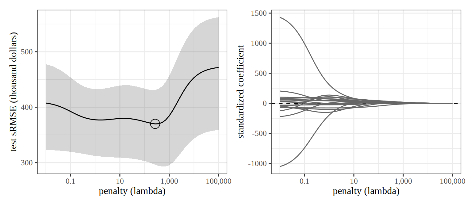
The lowest test sample root mean squared error (sRMSE), 370 thousand dollars (95% confidence interval [296, 431]), is at \(\regpar \approx\) 268. The sRMSE is the square root of the sample mean squared error, so it is in the units of Salary (why we report sRMSE). Each interval is the mean of the test players’ squared errors plus or minus 1.98 standard errors, the \(t\) interval for a mean, with its endpoints square-rooted. The lowest test error was also picked from 50 candidates by looking at the test half, so it is optimistic about the error of the chosen \(\regpar\). An honest error for the chosen \(\regpar\) needs players that took no part in choosing it. The penalty trades a little bias for a lower variance, and a model with 19 correlated predictors and 131 training players has variance to give up. Figure 1 shows the test error and the coefficients for every \(\regpar\).
Figure 1: Ridge regression on the Hitters data. Left: test sample root mean squared error (sRMSE) against the penalty, with a shaded 95% confidence interval and the lowest value marked. Right: each standardized coefficient against the penalty, one line per predictor.
ExrExercise 3 (Predicting baseball salaries with ridge regression (part 3))
Exercise 3 (Predicting baseball salaries with ridge regression (part 3)) Use the setup of Exercise 1.
How does the test error of that \(\regpar\) compare with that of \(\regpar \approx 0\)?
# Every model predicts the same test players, so differences are taken player by player.diff_small<-mean_ci(sq_err[, 1]-sq_err[, which.min(test_mse)])small_covers_0<-diff_small[["lower"]]<=0&&diff_small[["upper"]]>=0
Almost no penalty, \(\regpar = 10^{-2}\), gives a test sRMSE of 408 ([323, 478]), which is 10% higher than the lowest. The intervals for different \(\regpar\) overlap because they use the same players, so compare errors player by player, in squared units: almost no penalty has an sMSE larger by 29,259 on average than the lowest-error penalty, with a 95% confidence interval of [-24,602, 83,119]. This interval includes 0, so on this split the improvement over almost no penalty is within what the choice of test players could produce, even though the penalty was picked because its test error was lowest.
ExrExercise 4 (Predicting baseball salaries with ridge regression (part 4))
Exercise 4 (Predicting baseball salaries with ridge regression (part 4)) Use the setup of Exercise 1.
How does the test error of that \(\regpar\) compare with that of predicting the trainingmean salary for every player?
Predicting the trainingmean salary for every player gives a test sRMSE of 474. Its sMSE is larger than that of the lowest-error penalty by 87,813 on average, with a 95% confidence interval of [24,199, 151,427]. This interval excludes 0. Both intervals reflect which players were in the test half, not which were in the training half, and both differences are optimistic for the same reason as the lowest error: the penalty was picked by looking at the test half.
ExrExercise 5 (Choose the ridge penalty by cross-validation on baseball salaries)
Exercise 5 (Choose the ridge penalty by cross-validation on baseball salaries) In Exercise 1 we chose \(\regpar\) by its error on the test half, so no player was left to estimate the error of the choice. Choose it using the training half alone instead.
Solution 5. The code standardizes the predictors once on the whole training half, as in Solution 1, so the held-out fold’s means and standard deviations take part in its scaling. That leaks a little information from each held-out fold into its own fit.
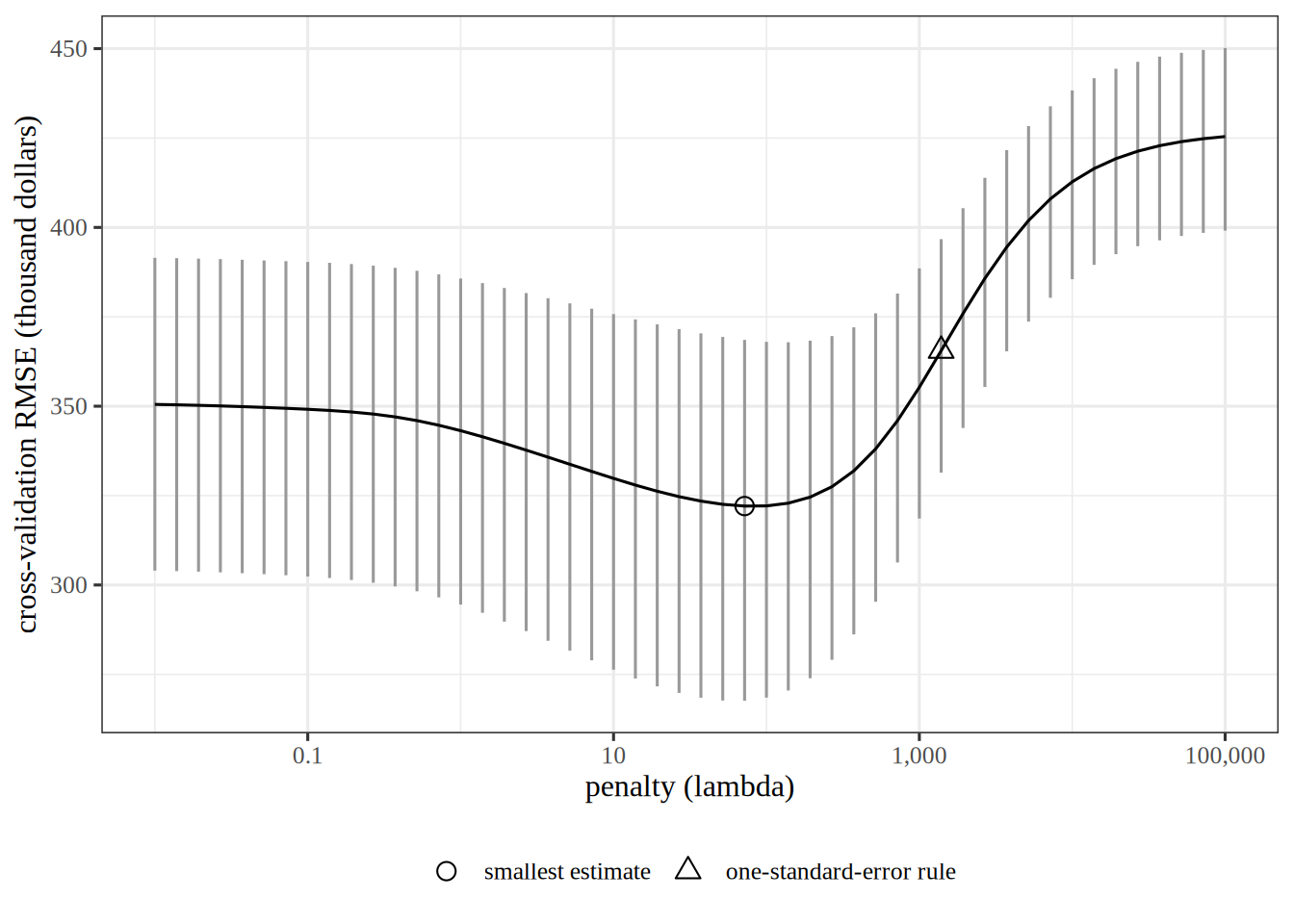
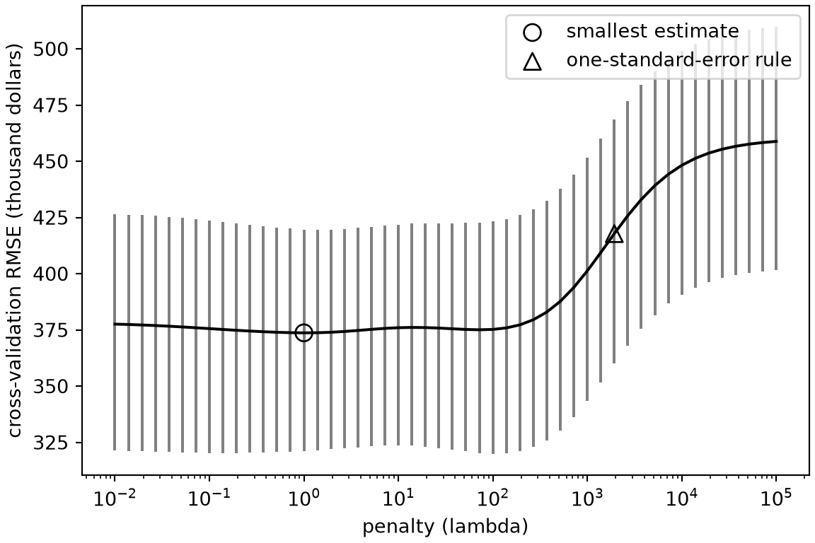
x_tr<-X[train, ]ytr<-y[train]k_cv<-10set.seed(2)fold<-sample(rep(seq_len(k_cv), length.out =length(train)))# The squared error of each training player when its fold is held out,# one column per penalty.cv_sq<-sapply(lambdas, function(l){sq<-numeric(length(ytr))for(finseq_len(k_cv)){held<-fold==fx_in<-x_tr[!held, ]b<-solve(t(x_in)%*%x_in+l*I0, t(x_in)%*%ytr[!held])sq[held]<-(ytr[held]-x_tr[held, ]%*%b)^2}sq})cv_est<-colMeans(cv_sq)# The fold-based standard error: the standard deviation of the ten fold sMSEs over sqrt(10).fold_mse<-apply(cv_sq, 2, function(sq)tapply(sq, fold, mean))cv_se<-apply(fold_mse, 2, sd)/sqrt(k_cv)
import matplotlib.pyplot as pltXtr_py, ytr_py = X_py[train_py], y_py[train_py]k_cv =10rng_cv = np.random.default_rng(2)fold_py = rng_cv.permutation(np.arange(len(ytr_py)) % k_cv)# The squared error of each training player when its fold is held out,# one column per penalty.cv_sq_py = np.empty((len(ytr_py), len(lams_py)))for f inrange(k_cv): held = fold_py == f x_in, ya = Xtr_py[~held], ytr_py[~held]for j, lam inenumerate(lams_py): b = np.linalg.solve(x_in.T @ x_in + lam * I0_py, x_in.T @ ya) cv_sq_py[held, j] = (ytr_py[held] - Xtr_py[held] @ b) **2cv_py = cv_sq_py.mean(axis=0)# The fold-based standard error: the standard deviation of the ten fold sMSEs over sqrt(10).fold_mse_py = np.array([cv_sq_py[fold_py == f].mean(axis=0) for f inrange(k_cv)])se_py = fold_mse_py.std(axis=0, ddof=1) / np.sqrt(k_cv)
The numbers in the later parts of this solution are from the R split and its folds.
ExrExercise 6 (Choose the ridge penalty by cross-validation on baseball salaries (part 2))
Exercise 6 (Choose the ridge penalty by cross-validation on baseball salaries (part 2)) Use the setup of Exercise 5.
The training half alone chose both penalties, so the test half gives an error estimate for each that the choice did not use. The test RMSEs are 376 at the smallest estimate and 394 at the larger penalty.
ExrExercise 8 (Choose the ridge penalty by cross-validation on baseball salaries (part 4))
Exercise 8 (Choose the ridge penalty by cross-validation on baseball salaries (part 4)) Use the setup of Exercise 5.
Solution 8. The two penalties of Solution 6 differ by 43 in cross-validation RMSE and by 19 in test RMSE, so the larger penalty has the higher test error on this split. The rule trades a small increase in cross-validation error for a simpler, more heavily shrunken fit, and the cross-validation error alone cannot say which is better.
3 The lasso
ExrExercise 9 (The coordinate update for the lasso (part 5))
Solution 9. With \(\regpar = 0\), \(S_0(c) = c\), and the update is \(\coef{j} = \dprod{\design_{\cdot j}}{r_j}/\norm{\design_{\cdot j}}^2\). That update is the least squarescoefficient of the residual\(r_j\) on the single feature\(\design_{\cdot j}\). Coordinate descent then amounts to fitting each feature to what the others leave unexplained, in turn.
Now apply it. We use the same training half and standardized predictors as Exercise 1. We center the salaries on the training mean, which takes care of the intercept.
# Soft-thresholding shrinks z toward zero by tau,# and returns exactly zero when |z| <= tau, which makes the lasso sparse.def soft_py(z, tau):return np.sign(z) *max(abs(z) - tau, 0.0)def lasso_cd_py(X, y, lam, tol=1e-8, max_sweeps=5000): beta = np.zeros(X.shape[1]) col_ss = (X**2).sum(axis=0) # ||X_j||^2 for each column, which does not changefor _ inrange(max_sweeps): biggest_change =0.0for j inrange(X.shape[1]):# Partial residual: y minus every feature's contribution except feature j's. r_j = y - X @ beta + X[:, j] * beta[j] new = soft_py(X[:, j] @ r_j, lam /2) / col_ss[j] biggest_change =max(biggest_change, abs(new - beta[j])) beta[j] = new# Stop once a full sweep barely moves any coefficient.if biggest_change < tol:breakreturn beta# Drop the intercept column of X_py; centering y takes care of the intercept.Xtr_py = X_py[train_py, 1:]ytr_py = y_py[train_py] - y_py[train_py].mean()lam_max_py =2* np.abs(Xtr_py.T @ ytr_py).max() # the smallest lambda that zeroes every coefficientlams_lasso_py = lam_max_py *10.0** np.linspace(-4, 0, 30)nonzero_py, mse_lasso_py = [], []for lam in lams_lasso_py: b = lasso_cd_py(Xtr_py, ytr_py, lam) nonzero_py.append(int((b !=0).sum())) pred = y_py[train_py].mean() + X_py[test_py, 1:] @ b mse_lasso_py.append(np.mean((y_py[test_py] - pred) **2))print("nonzero coefficients at the smallest and largest lambda:", nonzero_py[0], nonzero_py[-1])
nonzero coefficients at the smallest and largest lambda: 19 0
print("lowest test MSE:", round(min(mse_lasso_py)), "with", nonzero_py[int(np.argmin(mse_lasso_py))], "nonzero coefficients")
lowest test MSE: 106793 with 14 nonzero coefficients
# Soft-thresholding shrinks z toward zero by tau,# and returns exactly zero when |z| <= tau, which makes the lasso sparse.soft<-function(z, tau)sign(z)*pmax(abs(z)-tau, 0)lasso_cd<-function(x_mat, y, lambda, tol=1e-8, max_sweeps=5000){beta<-rep(0, ncol(x_mat))col_ss<-colSums(x_mat^2)# ||X_j||^2 for each column, which does not changefor(sinseq_len(max_sweeps)){biggest_change<-0for(jinseq_len(ncol(x_mat))){# Partial residual: y minus every feature's contribution except j's.r_j<-y-x_mat%*%beta+x_mat[, j]*beta[j]new<-soft(sum(x_mat[, j]*r_j), lambda/2)/col_ss[j]biggest_change<-max(biggest_change, abs(new-beta[j]))beta[j]<-new}# Stop once a full sweep barely moves any coefficient.if(biggest_change<tol)break}beta}# Drop the intercept column of x_mat; centering y takes care of the intercept.x_train<-Xs[train, ]ytr<-y[train]-mean(y[train])# The smallest lambda that zeroes every coefficient.lambda_max<-2*max(abs(crossprod(x_train, ytr)))lambdas_lasso<-lambda_max*10^seq(-4, 0, length.out =30)fits<-sapply(lambdas_lasso, function(l)lasso_cd(x_train, ytr, l))nonzero<-colSums(fits!=0)mse_lasso<-apply(fits, 2,function(b)mean((y[-train]-mean(y[train])-Xs[-train, ]%*%b)^2))print(nonzero[c(1, 30)])
# At a solution, the gradient of the squared error balances the penalty's slope:# 2 X_j'(y - Xb) = lambda * sign(b_j) when b_j is not zero,# and |2 X_j'(y - Xb)| <= lambda when b_j is zero.i_mid<-15b_mid<-fits[, i_mid]score<-2*crossprod(x_train, ytr-x_train%*%b_mid)kkt_gap<-max(abs(score[b_mid!=0]-lambdas_lasso[i_mid]*sign(b_mid[b_mid!=0])),pmax(abs(score[b_mid==0])-lambdas_lasso[i_mid], 0))stopifnot(kkt_gap<1e-5)fmt<-function(x)format(round(x), big.mark =",", scientific =FALSE)
The two languages split the players at random in different ways, so their numbers differ. The numbers below are from the R split.
With the smallest \(\regpar\) in the grid, all 19 coefficients are non-zero. With the largest, 0 are. The lowest test error, 141,389, comes with 9 non-zero coefficients. For comparison, ridge regression reached 136,857 in Solution 2, but it keeps every predictor.
As a check that coordinate descent has found the minimizer, the lasso’s optimality conditions hold at the middle \(\regpar\) in the grid to within \(10^{-5}\). The three parts of the coordinate update solution encode these conditions: the penalty’s slope\(\regpar\,\sign(\coef{j})\) balances the gradient of the squared error for each non-zero coefficient, and the gradient is no larger than \(\regpar\) in absolute value for each zero one.
ExrExercise 10 (Count the zero coefficients of ridge and the lasso on baseball salaries)
Exercise 10 (Count the zero coefficients of ridge and the lasso on baseball salaries) Use the Hitters data and the training half of Exercise 1, with the predictors standardized and the salary centered by the training mean. For \(\regpar = 10^2, 10^{2.5}, \dots, 10^5\), fitridge regression with the closed-form solution of this chapter, and fit the lasso by the coordinate descent of the lasso coordinate update.
import numpy as npimport pandas as pdhz_py = pd.read_csv("data/hitters.csv").dropna()hz_x = pd.get_dummies(hz_py.drop(columns="Salary"), drop_first=True)hz_names =list(hz_x.columns)hz_x = hz_x.to_numpy(dtype=float)hz_y = hz_py["Salary"].to_numpy()rng = np.random.default_rng(1)hz_train = rng.permutation(len(hz_y))[: len(hz_y) //2]# Standardize with the training half's mean and standard deviation, and center# the salary, so that no intercept needs to be fit or penalized.xt = hz_x[hz_train]xt = (xt - xt.mean(axis=0)) / xt.std(axis=0, ddof=1)yt = hz_y[hz_train] - hz_y[hz_train].mean()def ridge_zero_py(lam):return np.linalg.solve(xt.T @ xt + lam * np.eye(xt.shape[1]), xt.T @ yt)def lasso_zero_py(lam, sweeps=200):# Coordinate descent: each coefficient in turn is set to the soft-thresholded# correlation of its feature with the partial residual, over the feature's# sum of squares. b = np.zeros(xt.shape[1])for _ inrange(sweeps):for j inrange(xt.shape[1]): r = yt - xt @ b + xt[:, j] * b[j] z = xt[:, j] @ r b[j] = np.sign(z) *max(abs(z) - lam /2, 0.0) / (xt[:, j] @ xt[:, j])return blams_py =10.0** np.arange(2, 5.5, 0.5)
hz<-na.omit(read.csv("data/hitters.csv"))hz_x<-model.matrix(Salary~., data =hz)[, -1]set.seed(1)hz_train<-sample(nrow(hz), nrow(hz)/2)# Standardize with the training half's mean and standard deviation, and center# the salary, so that no intercept needs to be fit or penalized.xt<-scale(hz_x[hz_train, ], center =colMeans(hz_x[hz_train, ]), scale =apply(hz_x[hz_train, ], 2, sd))yt<-hz$Salary[hz_train]-mean(hz$Salary[hz_train])ridge_zero<-function(lambda){drop(solve(crossprod(xt)+lambda*diag(ncol(xt)), crossprod(xt, yt)))}lasso_zero<-function(lambda, sweeps=200){# Coordinate descent: each coefficient in turn is set to the soft-thresholded# correlation of its feature with the partial residual, over the feature's# sum of squares.b<-rep(0, ncol(xt))for(sinseq_len(sweeps)){for(jinseq_len(ncol(xt))){r<-yt-xt[, -j, drop =FALSE]%*%b[-j]z<-sum(xt[, j]*r)b[j]<-sign(z)*max(abs(z)-lambda/2, 0)/sum(xt[, j]^2)}}b}lams<-10^seq(2, 5, by =0.5)
The two languages split the players at random in different ways, so their counts differ. The numbers in the later parts of this solution are from the R split.
ExrExercise 11 (Count the zero coefficients of ridge and the lasso on baseball salaries (part 2))
Exercise 11 (Count the zero coefficients of ridge and the lasso on baseball salaries (part 2)) Use the setup of Exercise 10.
For each \(\regpar\), count the coefficients that are exactly zero in each fit.
pd.DataFrame({"lambda": lams_py.round(),"ridge_zeros": [int(np.sum(ridge_zero_py(l) ==0)) for l in lams_py],"lasso_zeros": [int(np.sum(lasso_zero_py(l) ==0)) for l in lams_py],})
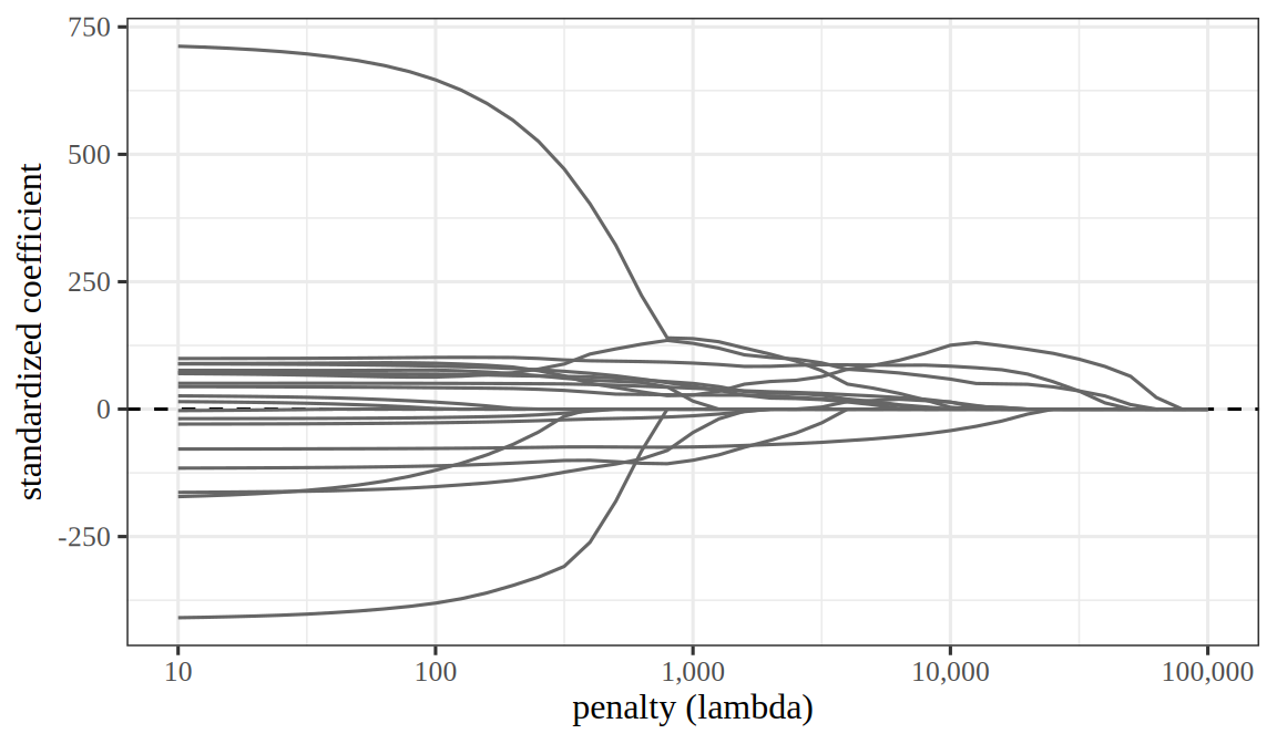
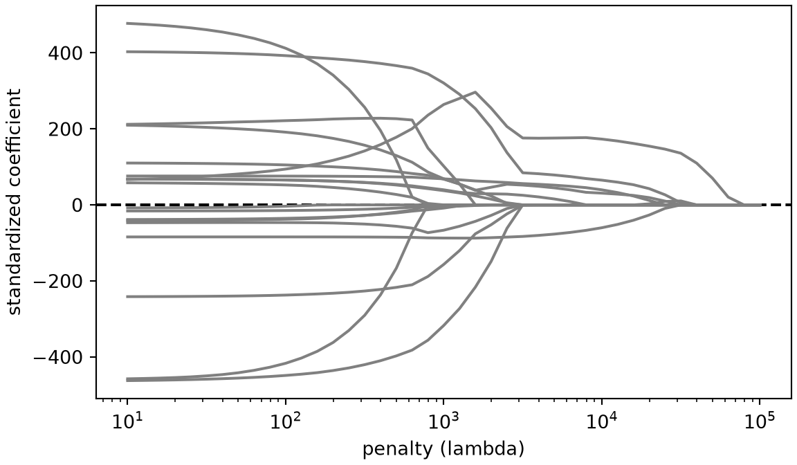
Ridge leaves every coefficient nonzero at every \(\regpar\) in the grid, so the count of zeros stays at 0. The lasso’s count climbs from 1 of the 19 coefficients at \(\regpar = 10^2\) to all 19 at \(\regpar = 10^5\). Figure 3 plots each lasso coefficient against \(\regpar\) on a finer grid, the counterpart of the ridge paths in Figure 1: the ridge curves shrink smoothly toward zero, while the lasso curves reach zero exactly, one after another.
Show code
# Fit the lasso of the R block at 41 penalties, evenly spaced on a log scale# from 10 to 100,000, so the paths are smooth between the grid of the exercise.path_lams<-10^seq(1, 5, by =0.1)n_coef<-ncol(xt)one_fit<-numeric(n_coef)lasso_path<-vapply(path_lams, lasso_zero, one_fit)n_lams<-length(path_lams)first_fit<-lasso_path[, 1]last_fit<-lasso_path[, n_lams]nonzero_first<-sum(first_fit!=0)nonzero_last<-sum(last_fit!=0)lambda_column<-rep(path_lams, each =n_coef)coef_names<-colnames(xt)predictor_column<-rep(coef_names, times =n_lams)coefficient_column<-as.vector(lasso_path)lasso_path_df<-tibble::tibble( lambda =lambda_column, predictor =predictor_column, coefficient =coefficient_column)lambda_labels<-scales::label_number(big.mark =",", drop0trailing =TRUE)lasso_path_df|>ggplot2::ggplot()+ggplot2::aes(x =lambda, y =coefficient, group =predictor)+ggplot2::geom_hline(yintercept =0, linetype ="dashed")+ggplot2::geom_line(colour ="grey40")+ggplot2::scale_x_log10(labels =lambda_labels)+ggplot2::labs(x ="penalty (lambda)", y ="standardized coefficient")
Show code
import matplotlib.pyplot as plt# Fit the lasso of the Python block at 41 penalties, evenly spaced on a log# scale from 10 to 100,000, so the paths are smooth between the grid of the exercise.path_lams_py =10.0** np.arange(1, 5.05, 0.1)lasso_path_py = np.array([lasso_zero_py(l) for l in path_lams_py])nonzero_first_py =int(np.sum(lasso_path_py[0] !=0))nonzero_last_py =int(np.sum(lasso_path_py[-1] !=0))fig, ax = plt.subplots(figsize=(6, 3.5), layout="constrained")ax.axhline(0, linestyle="--", color="black");ax.plot(path_lams_py, lasso_path_py, color="grey");ax.set_xscale("log");ax.set_xlabel("penalty (lambda)");ax.set_ylabel("standardized coefficient");plt.show()
Figure 3: Each curve shows the lassocoefficient of one of the 19 standardized predictors of Salary against \(\regpar\) on a logarithmic axis. Each tab fits the lasso to its own language’s training half of the Hitters data, and the two languages split the players differently, so the tabs’ paths differ. At \(\regpar = 10\), 19 of the coefficients are non-zero on the R tab and 19 on the Python tab; at \(\regpar = 10^5\), 0 are non-zero on the R tab and 0 on the Python tab.
# The standardized training half xt and centered salary yt are from the previous solution.ridge_fit<-function(x, y, lambda){drop(solve(crossprod(x)+lambda*diag(ncol(x)), crossprod(x, y)))}lasso_fit<-function(x, y, lambda, sweeps=100){b<-numeric(ncol(x))r<-yss<-colSums(x^2)for(sinseq_len(sweeps)){for(jinseq_len(ncol(x))){z<-sum(x[, j]*r)+ss[j]*b[j]b_new<-sign(z)*max(abs(z)-lambda/2, 0)/ss[j]r<-r-x[, j]*(b_new-b[j])b[j]<-b_new}}b}set.seed(2)folds<-sample(rep(1:10, length.out =nrow(xt)))lams_cv<-10^seq(1.5, 4.5, by =0.5)cv_estimate<-function(fit){sapply(lams_cv, function(lambda){sq<-numeric(nrow(xt))for(fin1:10){held<-folds==fb<-fit(xt[!held, ], yt[!held], lambda)sq[held]<-(yt[held]-xt[held, ]%*%b)^2}mean(sq)})}cv_ridge<-cv_estimate(ridge_fit)cv_lasso<-cv_estimate(lasso_fit)data.frame( lambda =round(lams_cv), ridge_cv_rmse =round(sqrt(cv_ridge)), lasso_cv_rmse =round(sqrt(cv_lasso)))
# The standardized training half xt and centered salary yt are from the previous solution.def ridge_fit_py(x, y, lam):return np.linalg.solve(x.T @ x + lam * np.eye(x.shape[1]), x.T @ y)def lasso_fit_py(x, y, lam, sweeps=100): b = np.zeros(x.shape[1]) r = y.copy() ss = (x **2).sum(axis=0)for _ inrange(sweeps):for j inrange(x.shape[1]): z = x[:, j] @ r + ss[j] * b[j] b_new = np.sign(z) *max(abs(z) - lam /2, 0.0) / ss[j] r -= x[:, j] * (b_new - b[j]) b[j] = b_newreturn bfolds_py = np.random.default_rng(2).permutation(np.arange(len(yt)) %10)lams_cv_py =10.0** np.arange(1.5, 4.6, 0.5)def cv_estimate_py(fit): out = []for lam in lams_cv_py: sq = np.empty(len(yt))for f inrange(10): held = folds_py == f b = fit(xt[~held], yt[~held], lam) sq[held] = (yt[held] - xt[held] @ b) **2 out.append(sq.mean())return np.array(out)cv_ridge_py = cv_estimate_py(ridge_fit_py)cv_lasso_py = cv_estimate_py(lasso_fit_py)pd.DataFrame({"lambda": lams_cv_py.round(),"ridge_cv_rmse": np.sqrt(cv_ridge_py).round(),"lasso_cv_rmse": np.sqrt(cv_lasso_py).round(),})
The two languages split the players at random in different ways, so their numbers differ. The numbers in the later parts of this solution are from the R split.
ExrExercise 15 (Choose the lasso penalty by cross-validation on baseball salaries (part 2))
Exercise 15 (Choose the lasso penalty by cross-validation on baseball salaries (part 2)) Use the setup of Exercise 14.
For each method, find the \(\regpar\) with the smallest estimate, refit on the whole training half, and compute the root mean squared error on the test half.
Cross-validation chooses \(\regpar =\) 100 for ridge regression and \(\regpar =\) 3162 for the lasso. The test root mean squared error is 374 thousand dollars for ridge regression and 378 for the lasso.
ExrExercise 16 (Choose the lasso penalty by cross-validation on baseball salaries (part 3))
Exercise 16 (Choose the lasso penalty by cross-validation on baseball salaries (part 3)) Use the setup of Exercise 14.
How many lasso coefficients are exactly zero at the chosen \(\regpar\)?
Solution 17. Ridge regression has the lower test error, 374 thousand dollars against 378. The test half played no part in choosing either penalty, so these two errors compare the methods fairly.
4 Principal components regression and partial least squares
ExrExercise 18 (Predict baseball salaries from a few combinations of the predictors)
Exercise 18 (Predict baseball salaries from a few combinations of the predictors) Ridge regression and the lasso keep all 19 predictors of the Hitters data and penalize their coefficients. Here we instead replace the predictors by \(M\)linear combinations of them, and fit least squares on those combinations alone. We build the combinations in two ways.
Greatest variance of the predictors. Take the first \(M\) directions, in order, along which the standardized training predictors vary most. These are the first \(M\) right singular vectors of the standardized training predictor matrix (see principal component analysis). Each combination weights the predictors by the entries of one singular vector.
Relation to the salary. Weight each standardized predictor by its simple regression coefficient on the centered salary, and add the weighted predictors to make the first combination. Subtract from every predictor the part of it that the first combination explains, by regressing each predictor on the combination and keeping the residuals. Build the second combination from the residuals in the same way, and repeat.
Use the training half and the standardized predictors of Exercise 1, and the ten folds of Exercise 5. For each way and each \(M = 0, 1, \dots, 19\), compute the 10-fold cross-validation estimate. Take \(M = 0\) to predict the training mean salary for every player.
For the second way, the residual of a predictor after regressing on a combination \(\vz\) is \(x_j - \vz\,\dprod{\vz}{x_j}/\dprod{\vz}{\vz}\), so after \(m - 1\) combinations the residual predictors are \(\design\prod_{k<m}\paren{I - \vphi_k\tp{\vp_k}}\), where \(\vphi_k\) holds the weights of combination \(k\) and \(\vp_k\) the regressioncoefficients of the predictors on it. That lets the code express every combination in the original standardized predictors.
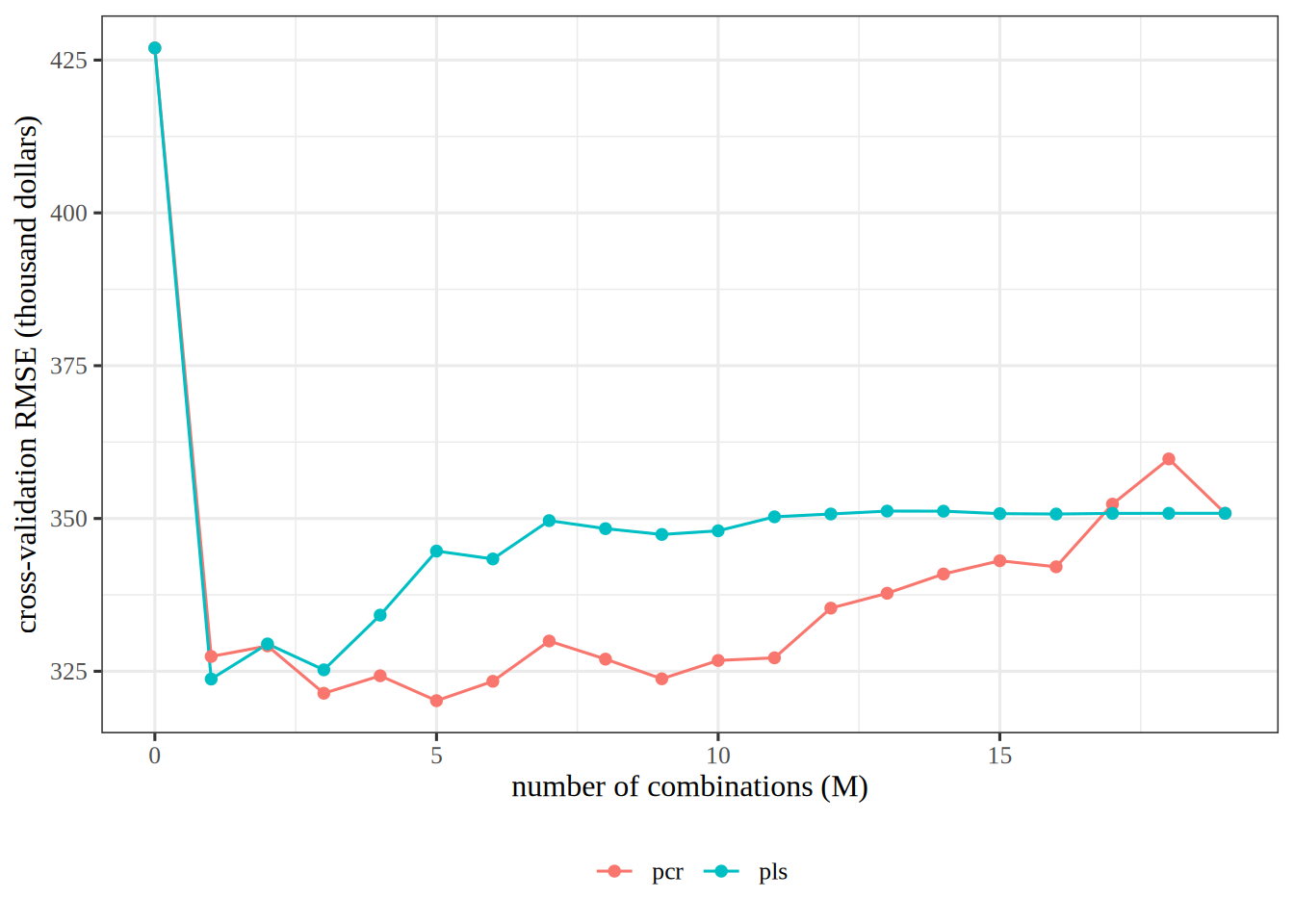
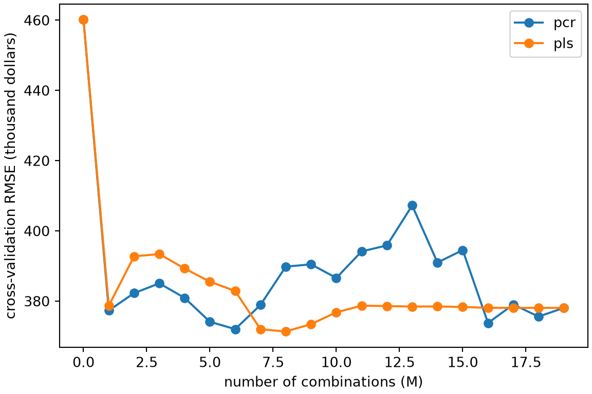
Figure 4: How each of the two ways scores against the number of combinations used.
xs_tr<-Xs[train, ]y_tr<-y[train]d<-ncol(xs_tr)pls_dirs<-function(x, y, m){# Columns are the weights of each combination on the original predictors.proj<-diag(ncol(x))xk<-xout<-matrix(0, ncol(x), m)for(kinseq_len(m)){phi<-drop(crossprod(xk, y))/colSums(xk^2)z<-drop(xk%*%phi)p<-drop(crossprod(xk, z))/sum(z^2)out[, k]<-proj%*%phiproj<-proj%*%(diag(ncol(x))-outer(phi, p))xk<-xk-outer(z, p)}out}fit_predict<-function(x, y, m, method, x_new){x_bar<-colMeans(x)x_c<-sweep(x, 2, x_bar)y_c<-y-mean(y)if(m==0){return(rep(mean(y), nrow(x_new)))}w<-if(method=="pcr")svd(x_c, nu =0, nv =m)$velsepls_dirs(x_c, y_c, m)z<-x_c%*%wbeta<-drop(w%*%solve(crossprod(z), crossprod(z, y_c)))mean(y)+drop(sweep(x_new, 2, x_bar)%*%beta)}methods<-c("pcr", "pls")cv_sq_dr<-lapply(setNames(methods, methods), function(meth){sq<-matrix(0, length(y_tr), d+1)for(finseq_len(k_cv)){held<-fold==ffor(min0:d){pred<-fit_predict(xs_tr[!held, ], y_tr[!held], m, meth, xs_tr[held, , drop =FALSE])sq[held, m+1]<-(y_tr[held]-pred)^2}}sq})library(ggplot2)cv_curves<-do.call(rbind, lapply(methods, function(meth){data.frame(method =meth, m =0:d, cv_rmse =sqrt(colMeans(cv_sq_dr[[meth]])))}))ggplot(cv_curves, aes(m, cv_rmse, colour =method))+geom_line()+geom_point()+labs(x ="number of combinations (M)", y ="cross-validation RMSE (thousand dollars)", colour =NULL)+theme(legend.position ="bottom")
xs_tr_py = X_py[train_py, 1:]y_tr_py = y_py[train_py]d_py = xs_tr_py.shape[1]def pls_dirs_py(x, y, m):# Columns are the weights of each combination on the original predictors. proj = np.eye(x.shape[1]) xk = x out = np.zeros((x.shape[1], m))for k inrange(m): phi = (xk.T @ y) / (xk **2).sum(axis=0) z = xk @ phi p = (xk.T @ z) / (z @ z) out[:, k] = proj @ phi proj = proj @ (np.eye(x.shape[1]) - np.outer(phi, p)) xk = xk - np.outer(z, p)return outdef fit_predict_py(x, y, m, method, x_new): x_bar = x.mean(axis=0) x_c, y_c = x - x_bar, y - y.mean()if m ==0:return np.full(len(x_new), y.mean()) w = (np.linalg.svd(x_c, full_matrices=False)[2][:m].Tif method =="pcr"else pls_dirs_py(x_c, y_c, m)) z = x_c @ w beta = w @ np.linalg.solve(z.T @ z, z.T @ y_c)return y.mean() + (x_new - x_bar) @ betamethods_py = ["pcr", "pls"]cv_sq_dr_py = {meth: np.empty((len(y_tr_py), d_py +1)) for meth in methods_py}for meth in methods_py:for f inrange(k_cv): held = fold_py == ffor m inrange(d_py +1): pred = fit_predict_py(xs_tr_py[~held], y_tr_py[~held], m, meth, xs_tr_py[held]) cv_sq_dr_py[meth][held, m] = (y_tr_py[held] - pred) **2fig, ax = plt.subplots(figsize=(6, 4), layout="constrained")for meth in methods_py: ax.plot(range(d_py +1), np.sqrt(cv_sq_dr_py[meth].mean(axis=0)), marker="o", label=meth);ax.set_xlabel("number of combinations (M)");ax.set_ylabel("cross-validation RMSE (thousand dollars)");ax.legend();plt.show()
Figure 4 plots the score of each way against the number of combinations.
The numbers in the later parts of this solution are from the R split and its folds. With \(M = 19\) both ways give the least squares fit on all the predictors.
ExrExercise 19 (Predict baseball salaries from a few combinations of the predictors (part 2))
Exercise 19 (Predict baseball salaries from a few combinations of the predictors (part 2)) Use the setup of Exercise 18.
For each way, which \(M\) has the smallest estimate?
G. James, D. Witten, T. Hastie, R. Tibshirani, and J. Taylor, An introduction to statistical learning: With applications in Python. Springer, 2023. doi: 10.1007/978-3-031-38747-0.
[2]
G. James, D. Witten, T. Hastie, R. Tibshirani, and J. Taylor, “ISLP labs: Lab notebooks for an introduction to statistical learning with applications in python.” GitHub repository, BSD 2-Clause license, 2023. Available: https://github.com/intro-stat-learning/ISLP_labs
[3]
G. James, D. Witten, T. Hastie, and R. Tibshirani, An introduction to statistical learning with applications in R, 2nd ed. Springer, 2021. Available: https://www.statlearning.com/