Resampling Methods

Published

Last modified: 2026-11-19

Adapted from Kameron Decker Harris’ 2022 weekly notes.

1 Resampling methods

Resampling methods draw repeated samples from the data we have, and fit the same model again to each one. Comparing the fits shows what a single fit cannot, such as how well the model predicts new data.

2 Holding out a validation set

The simplest approach splits the data once, into the three parts in Figure 1. We fit each candidate model on the training set, choose the candidate with the smallest validation error, and report the chosen model’s test error.

Figure 1: One rectangle cut into three parts, left to right: a wide part labeled Train, a narrower part labeled Val, and a narrow part labeled Test.
A single rectangle divided by two vertical lines into three parts, left to right: a wide part labeled Train, a narrower part labeled Val, and a narrow part labeled Test.

With only one candidate, nothing is chosen. A validation set is then not needed, and the two-part split in Figure 2 suffices.

Figure 2: One rectangle cut into two parts: a wide part labeled Train on the left and a narrower part labeled Test on the right.
A single rectangle divided by a vertical line into two parts: a wide part labeled Train on the left and a narrower part labeled Test on the right.

2.1 Weighing a single split

A single split assumes that the observations are independent and identically distributed. Even then, it has three drawbacks:

VideosWatch

Hastie and Tibshirani describe the validation-set approach, from 8:11, and its drawbacks, from 13:14 [1], video 5.1.

VideosWatch

Abu-Mostafa covers model selection with a validation set in his lecture on validation, from 30:47 [2], Lecture 13.

VideosWatch

The CS229 lecture covers data splits, models and cross-validation [3], Lecture 8.

VideosWatch

Lall compares validation approaches in his EE104 lecture on validation, from 14:20 [4], Lecture 4.

3 K-fold cross-validation

\(K\)-fold cross-validation splits the data into \(K\) folds. This \(K\) is not the number of neighbors in \(K\)-nearest neighbors. Both names are standard, so the letter is reused. Figure 3 shows \(K = 4\).
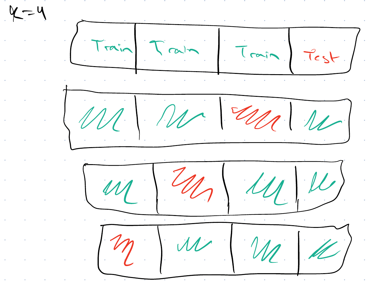
Figure 3: Four bars, each cut into four folds, for \(K = 4\). The last fold of the first bar is the test fold. In each of the other three bars a different one of the first three folds is marked in red as the test fold, and the other three are marked in green.
Four hand-drawn bars, each divided into four blocks, for K equal to 4. The first bar is labeled Train, Train, Train, Test, so the last block is the test block. In each of the next three bars a different one of the first three blocks is marked in red as the test block, and the other three blocks are marked in green as training blocks.

The test fold rotates through the \(K\) folds. Each turn fits the model on the other \(K - 1\) folds and scores it on the test fold. The \(K\)-fold cross-validation estimate of the risk combines the \(K\) scores. When the folds have the same size, the cross-validation estimate is the sample mean of the \(K\) scores. Every observation is scored once, so the cross-validation estimate varies less than the validation error of a single split. The price is \(K\) fits instead of one.

Figure 4 runs \(K\)-fold cross-validation on the Auto data, one fold at a time. The mean squared errors of the folds vary from fold to fold, and their sample mean is the \(K\)-fold cross-validation estimate.

Show code
viewof krK = Inputs.select([2, 5, 10], {value: 5, label: "folds K"})
viewof krFold = Inputs.range([1, krK], {value: 1, step: 1, width: 300,
  label: "held-out fold"})
viewof krDegree = Inputs.range([1, 6], {value: 2, step: 1, width: 300, label: "degree"})
Show code
krFoldShown = Math.min(krFold, krK)
krPts = transpose(krPoints).map((d) => ({...d,
  role: d[`fold${krK}`] === krFoldShown ? "held out" : "trained on"}))
krCurve = transpose(krCurves).filter((d) =>
  d.k === krK && d.fold === krFoldShown && d.degree === krDegree)
krFoldMse = transpose(krMse).filter((d) => d.k === krK && d.degree === krDegree)
krEstimate = d3.mean(krFoldMse, (d) => d.mse)
krNow = krFoldMse.find((d) => d.fold === krFoldShown)
krHeldCount = krPts.filter((d) => d.role === "held out").length
Show code
md`The degree-${krDegree} fit trains on ${krPts.length - krHeldCount} cars
and scores the ${krHeldCount} cars of fold ${krFoldShown}:
its MSE on that fold is **${krNow.mse.toFixed(1)}**.
The ${krK}-fold estimate, the mean of the ${krK} fold MSEs, is **${krEstimate.toFixed(1)}**.`
Show code
Plot.plot({
  ariaLabel: "Scatter plot of mpg against horsepower for the Auto cars, " +
    "the held-out fold in orange and the training folds in light blue, " +
    "with the polynomial fitted to the training folds drawn as a black curve.",
  width: 420, height: 300, grid: true,
  x: {label: "horsepower"}, y: {label: "mpg", domain: [5, 50]},
  color: {domain: ["trained on", "held out"], range: ["#9ecae1", "#e66101"],
    legend: true},
  marks: [
    Plot.dot(krPts, {x: "horsepower", y: "mpg", fill: "role", r: 2.5,
      sort: {channel: "fill", order: "descending"}}),
    Plot.line(krCurve, {x: "horsepower", y: "mpg", stroke: "black", strokeWidth: 2,
      clip: true})
  ]
})
Show code
Plot.plot({
  ariaLabel: "Bar chart of the MSE on each held-out fold, " +
    "the current fold in orange, with a horizontal line at their mean, " +
    "the K-fold estimate.",
  width: 260, height: 300, grid: true,
  x: {label: "held-out fold", type: "band"},
  y: {label: "MSE on the held-out fold (mpg²)"},
  marks: [
    Plot.barY(krFoldMse, {x: "fold", y: "mse",
      fill: (d) => d.fold === krFoldShown ? "#e66101" : "#bbbbbb"}),
    Plot.ruleY([krEstimate], {stroke: "black", strokeDasharray: "5,3"}),
    Plot.ruleY([0])
  ]
})
Figure 4: \(K\)-fold cross-validation of a polynomial regression of mpg on horsepower, on the 392 cars of the Auto data, one held-out fold at a time. Each fit trains on the other \(K - 1\) folds, drawn in light blue, and is scored on the held-out fold, drawn in orange. The website lets you choose \(K\), the held-out fold and the degree, and plots the MSE on every held-out fold, with a dashed line at their sample mean, the \(K\)-fold estimate. The handout shows the 5 folds of a degree-2 fit, whose 5-fold estimate is 19.4.

3.1 Leave-one-out cross-validation

Leave-one-out cross-validation is the extreme case \(K = n\), in which each fold holds a single observation.

Show code
viewof vvReps = Inputs.range([1, 10], {value: 1, step: 1, width: 300,
  label: "random repetitions shown"})
viewof vvMethods = Inputs.checkbox(
  ["validation set", "10-fold CV", "leave-one-out CV"],
  {value: ["validation set", "10-fold CV", "leave-one-out CV"], label: "estimates"})
Show code
vvRows = transpose(vvData).filter((d) => d.rep <= vvReps && vvMethods.includes(d.method))
Show code
Plot.plot({
  ariaLabel: "Estimates of the test mean squared error of mpg against polynomial degree, " +
    "one panel per method, one line per random repetition. " +
    "The validation-set lines spread widely, the 10-fold lines nearly coincide, " +
    "and leave-one-out is a single line.",
  width: 720, height: 280, marginLeft: 50, grid: true,
  fx: {label: null, domain: vvMethods},
  x: {label: "polynomial degree", ticks: d3.range(1, 11)},
  y: {label: "estimated test MSE (mpg²)", domain: [15, 28]},
  color: {type: "categorical", scheme: "Tableau10"},
  marks: [
    Plot.frame({stroke: "#ccc"}),
    Plot.line(vvRows, {fx: "method", x: "degree", y: "mse", z: "rep",
      stroke: "rep", strokeWidth: 1.5, clip: true}),
    Plot.dot(vvRows, {fx: "method", x: "degree", y: "mse", fill: "rep", r: 2.5, clip: true})
  ]
})
Figure 5: Three estimates of the test mean squared error of a polynomial regression of mpg on horsepower, for the 392 cars of the Auto data, by degree. Each validation-set line comes from a different random half-and-half split, and each 10-fold line comes from a different random assignment of the cars to folds. Leave-one-out has one line, because it involves no randomness. The handout shows all 10 repetitions; the website adds them one at a time with the slider. The analysis follows Figures 5.2 and 5.4 of An Introduction to Statistical Learning [5].

Figure 5 compares three estimates of the test mean squared error on the Auto data. For the degree-2 fit, the ten estimates from a random validation set run from 17.5 to 21, the ten 10-fold estimates run from 19.2 to 19.5, and leave-one-out cross-validation gives 19.2. Averaging over folds makes the 10-fold estimate far less variable than a single split.

VideosWatch

Abu-Mostafa explains leave-one-out cross-validation, from 49:03 [2], Lecture 13.

VideosWatch

Hastie and Tibshirani go through \(K\)-fold cross-validation in detail, from 0:55 [1], video 5.2.

VideosWatch

Starmer explains \(K\)-fold cross-validation [6].

VideosWatch

Abu-Mostafa explains \(K\)-fold cross-validation, from 1:06:25 [2], Lecture 13.

VideosWatch

Lall covers cross-validation in his EE104 lecture on validation, from 36:24 [4], Lecture 4.

ReadingRead

GeeksforGeeks explains cross-validation [7], including \(K\)-fold and leave-one-out.

ReadingRead

The University of Washington’s CSE 446 slides cover train-test splits and cross-validation [8], Lecture 5.

Back to top

References

[1]
T. Hastie, R. Tibshirani, and J. Taylor, “Statistical learning with python.” Stanford Online, lecture videos on YouTube, 2023. Available: https://www.youtube.com/playlist?list=PLoROMvodv4rPP6braWoRt5UCXYZ71GZIQ
[2]
Y. S. Abu-Mostafa, “Learning from data: CS 156 lectures.” Caltech, lecture videos on YouTube, 2012. Available: https://www.youtube.com/playlist?list=PLD63A284B7615313A
[3]
A. Ng et al., “CS229: Machine learning, autumn 2018.” Stanford Online, lecture videos on YouTube, 2018. Available: https://www.youtube.com/playlist?list=PLoROMvodv4rMiGQp3WXShtMGgzqpfVfbU
[4]
S. Lall, “EE104: Introduction to machine learning, 2020.” Stanford Online, lecture videos on YouTube, 2020. Available: https://www.youtube.com/playlist?list=PLoROMvodv4rN_Uy7_wmS051_q1d6akXmK
[5]
G. James, D. Witten, T. Hastie, and R. Tibshirani, An introduction to statistical learning with applications in R, 2nd ed. Springer, 2021. Available: https://www.statlearning.com/
[6]
J. Starmer, “Machine learning fundamentals: Cross validation.” StatQuest, video on YouTube, 2018. Available: https://www.youtube.com/watch?v=fSytzGwwBVw
[7]
GeeksforGeeks, “Cross validation in machine learning.” GeeksforGeeks, tutorial article, 2026. Available: https://www.geeksforgeeks.org/machine-learning/cross-validation-machine-learning/
[8]
N. Jaques, “CSE 446/546: Machine learning, lecture slides.” University of Washington, 2026. Accessed: Oct. 12, 2026. [Online]. Available: https://courses.cs.washington.edu/courses/cse446/26sp/schedule/lectures/