Multiclass Logistic Regression

Published

Last modified: 2026-11-19

Show code
# The Python chunks on this page import these packages; reticulate provisions them.
library(reticulate)
py_packages <- c(
  "numpy", "pandas", "statsmodels", "scipy", "scikit-learn", "matplotlib",
  "plotnine"
)
py_require(py_packages)

Adapted from Brian Hutchinson’s Fall 2025 lecture notes on multinomial logistic regression, reorganized as exercises, and drawing on Logan Sizemore’s Spring 2025 lectures for the redundant weight vector. This material was a section of the logistic regression page. Solution 12 corrects the spurious \(1/\nobs\) in the source’s multinomial gradient and flags the correction rather than fixing it silently.

1 Regressing a class code

ExrExercise 1 (What a numeric class code assumes)

Exercise 1 (What a numeric class code assumes) The Auto data record where each car was made as origin, coded \(1\) for American, \(2\) for European and \(3\) for Japanese. A label with more than two classes could be predicted by linear regression on such a code: fit a least-squares line to the code, and assign each car the class whose code is nearest its fitted value. That approach reuses a method we already have, so it is worth knowing whether it is sound.

TipHint

Compare the distances between the codes with what the three classes are.

State what this coding assumes about the three origins.

Solution 1. The coding of origin in the Auto data assumes two facts about the origins that the data do not supply:

  • An order. European lies between American and Japanese, so a car whose fitted value moves from \(1\) toward \(3\) passes through European on the way.
  • Even spacing. The step from American to European is the same size as the step from European to Japanese.

The origins are names with no order, so neither assumption is justified. Any of the \(3! = 6\) assignments of the codes \(1, 2, 3\) to the origins is as defensible as the one in the file, and a different assignment gives a different line and different predictions [1, Sec. 4.2].

ExrExercise 2 (Regressing the origin code on fuel economy)

Exercise 2 (Regressing the origin code on fuel economy) Use the Auto data and the origin code of Exercise 1, with fuel economy mpg as the only feature. Fit a least-squares line of the code on mpg, in R or Python, and round each fitted value to the nearest of \(1, 2, 3\) to get a predicted origin.

TipHint

Fit models with tidymodels shows linear_reg() in R, and Fit and inspect a model with statsmodels shows sm.OLS in Python. Recode, count and combine data frames shows how to tally the values of a variable.

Report how many cars the line predicts to be of each origin.

Solution 2.

Show code
# Read the Auto data; `origin` holds the codes 1, 2 and 3.
cc_auto <- readr::read_csv("data/auto.csv", show_col_types = FALSE)

# Fit a least-squares line to the code, treating the code as a number.
cc_fit <- parsnip::linear_reg() |>
  parsnip::fit(origin ~ mpg, data = cc_auto)

# Round each fitted value `.pred` to the nearest code,
# then move a value below 1 or above 3 to the nearest end.
cc_aug <- cc_fit |>
  parsnip::augment(new_data = cc_auto) |>
  dplyr::mutate(
    pred = round(.pred),
    pred = pmax(pred, 1),
    pred = pmin(pred, 3)
  )

# Count the cars predicted to be of each origin.
cc_aug |> dplyr::count(pred)
Show code
import pandas as pd
import statsmodels.api as sm

# Read the Auto data; `origin` holds the codes 1, 2 and 3.
cc_auto = pd.read_csv("data/auto.csv")

# Fit a least-squares line to the code, treating the code as a number.
cc_X = sm.add_constant(cc_auto["mpg"])
cc_fit = sm.OLS(cc_auto["origin"], cc_X).fit()

# Round each fitted value to the nearest code,
# then move a value below 1 or above 3 to the nearest end.
cc_pred = cc_fit.fittedvalues.round().clip(1, 3)

# Count the cars predicted to be of each origin.
print(cc_pred.value_counts().sort_index())
1.0    193
2.0    190
3.0      9
Name: count, dtype: int64

The line predicts 193 cars to be American, 190 European and 9 Japanese, while the data hold only 68 European cars. European is coded between the other two origins, so the line predicts European for every car whose fitted value is nearer \(2\) than \(1\) or \(3\).

ExrExercise 3 (Changing the class code)

Exercise 3 (Changing the class code) Use the Auto data and the line of Exercise 2, but recode origin as \(1\) for European, \(2\) for American and \(3\) for Japanese. Refit the least-squares line to the new code, round its fitted values as before, and translate each predicted code back to an origin.

TipHint

Recode, count and combine data frames shows how to recode values.

Report how many cars get a different predicted origin from the one in Solution 2.

Solution 3. Swapping the codes \(1\) and \(2\) twice gives back the original codes, so one lookup both recodes the origins and translates the predicted codes back.

Show code
# Swap the codes of American (1) and European (2); Japanese stays 3.
cc_swap <- c(2, 1, 3)
cc_auto2 <- cc_auto |>
  dplyr::mutate(code = cc_swap[origin])

# Refit the line to the new code, and round as before.
cc_fit2 <- parsnip::linear_reg() |>
  parsnip::fit(code ~ mpg, data = cc_auto2)
cc_aug2 <- cc_fit2 |>
  parsnip::augment(new_data = cc_auto2) |>
  dplyr::mutate(
    code_pred = round(.pred),
    code_pred = pmax(code_pred, 1),
    code_pred = pmin(code_pred, 3),
    # The same swap translates a predicted code back to an origin.
    pred = cc_swap[code_pred]
  )

# Count the predicted origins, and the cars whose prediction changed.
cc_aug2 |> dplyr::count(pred)
Show code
cc_changed <- sum(cc_aug2$pred != cc_aug$pred)
cc_changed
[1] 199
Show code
# Swap the codes of American (1) and European (2); Japanese stays 3.
cc_swap = {1: 2, 2: 1, 3: 3}
cc_code = cc_auto["origin"].map(cc_swap)

# Refit the line to the new code, and round as before.
cc_fit2 = sm.OLS(cc_code, cc_X).fit()
cc_code_pred = cc_fit2.fittedvalues.round().clip(1, 3)

# The same swap translates a predicted code back to an origin.
cc_pred2 = cc_code_pred.map(cc_swap)

# Count the predicted origins, and the cars whose prediction changed.
print(cc_pred2.value_counts().sort_index())
1    392
Name: count, dtype: int64
Show code
print((cc_pred2 != cc_pred).sum())
199

The predicted origin changes for 199 of the 392 cars, although the data and the feature are the same and only the codes differ. With American now coded between the other two origins, the line predicts American for 392 of the 392 cars. A model for a label with unordered classes should treat the classes symmetrically. The rest of this page builds one that does.

2 The multinomial model

A logistic regression model has one coefficient vector, for a label with two classes. This section gives each of several classes its own coefficient vector and normalizes the exponentiated linear predictors into class probabilities. With two classes, that model reduces to logistic regression, and it is the output layer of multi-class neural network classifiers in the neural networks chapter.

ExrExercise 4 (More than two classes)

Exercise 4 (More than two classes) Logistic regression gives the label two classes and one coefficient vector. For \(C\) classes, give each class \(m\) its own coefficient vector \(B_m\) and set

\[P(Y = m \mid \vx) = \frac{\expf{\tp{B_m} \vx}} {\sum_k \expf{\tp{B_k} \vx}},\]

where the sum runs over all \(C\) classes.

Set \(C = 2\), label the two classes \(0\) and \(1\) as in logistic regression, and show that this expression reduces to \(P(\Outvar = 1 \mid \vx) = \sigmoidf{\dprod{\vcoef}{\vx}}\). Express \(\vcoef\) in terms of \(B_0\) and \(B_1\).

Solution 4. With two classes the sum in the denominator has two terms. Divide the numerator and the denominator by \(\e{\tp{B_1} \vx}\):

\[ \begin{aligned} P(Y = 1 \mid \vx) &= \frac{\e{\tp{B_1} \vx}}{\e{\tp{B_0} \vx} + \e{\tp{B_1} \vx}} && \text{(the model with $C = 2$)} \\ &= \frac{\e{\tp{B_1} \vx} / \e{\tp{B_1} \vx}}{\paren{\e{\tp{B_0} \vx} + \e{\tp{B_1} \vx}} / \e{\tp{B_1} \vx}} && \text{(divide numerator and denominator)} \\ &= \frac{1}{\paren{\e{\tp{B_0} \vx} + \e{\tp{B_1} \vx}} / \e{\tp{B_1} \vx}} && \text{(a number divided by itself is $1$)} \\ &= \frac{1}{\e{\tp{B_0} \vx} / \e{\tp{B_1} \vx} + 1} && \text{(divide each term of the sum)} \\ &= \frac{1}{\e{\tp{B_0} \vx - \tp{B_1} \vx} + 1} && \text{(quotient of exponentials)} \\ &= \frac{1}{\e{-\paren{\tp{B_1} \vx - \tp{B_0} \vx}} + 1} && \text{(factor out $-1$)} \\ &= \frac{1}{\e{-\tp{\paren{B_1 - B_0}} \vx} + 1} && \text{(factor out $\vx$)} \\ &= \frac{1}{1 + \e{-\tp{\paren{B_1 - B_0}} \vx}} && \text{(reorder the sum)} \\ &= \sigmoidf{\tp{\paren{B_1 - B_0}}\vx} && \text{(definition of the logistic function)}. \end{aligned} \]

So \(\vcoef = B_1 - B_0\): the single coefficient vector of the binary model is the difference between the two class coefficient vectors, not either vector alone.

This difference is why every logistic regression coefficient compares the two classes: by the odds-ratio corollary, \(\e{\coef{j}}\) is an odds ratio, and the odds of class \(1\) are its probability divided by the probability of class \(0\).

DefDefinition 1 (Softmax function)

Definition 1 (Softmax function) The softmax function maps a vector of scores \(\vz = \pt{z_1, \dots, z_C}\) in \(\reals^C\) to the vector \(\operatorname{softmax}(\vz)\) in \(\reals^C\) whose \(m\)th entry is

\[ \operatorname{softmax}(\vz)_m = \frac{\e{z_m}}{\sumto{k}{C} \e{z_k}}, \qquad m = 1, \dots, C \tag{1}\]

[2, Sec. 6.2.2.3], [3, Sec. 4.2]. Each entry is positive, and the entries sum to \(1\), so \(\operatorname{softmax}(\vz)\) is a probability mass function on the \(C\) classes. The denominator is the normalizer, written \(Z = \sumto{k}{C} \e{z_k}\).

ExmExample 1 (The softmax of three scores)

Example 1 (The softmax of three scores) Apply the softmax function to the scores \(\vz = \pt{1, 2, 3}\).

Show code
sm_z <- c(1, 2, 3)
sm_exp <- exp(sm_z)
sm_norm <- sum(sm_exp)
sm_prob <- sm_exp / sm_norm
# nolint start: undesirable_function_linter. A matrix.
rbind(exponential = sm_exp, softmax = sm_prob) |> round(3)
             [,1]  [,2]   [,3]
exponential 2.718 7.389 20.086
softmax     0.090 0.245  0.665
Show code
# nolint end
Show code
import numpy as np

z_sm = np.array([1.0, 2.0, 3.0])
exp_sm = np.exp(z_sm)
print(np.vstack([exp_sm, exp_sm / exp_sm.sum()]).round(3))
[[ 2.718  7.389 20.086]
 [ 0.09   0.245  0.665]]

The exponentials are 2.718, 7.389 and 20.086, and their sum is \(Z =\) 30.193. Dividing each exponential by \(Z\) gives the probabilities 0.090, 0.245 and 0.665, which sum to 1. The scores are equally spaced, but each probability is \(e \approx\) 2.718 times the one before it.

ReadingRead

GeeksforGeeks explains the softmax function [4].

DefDefinition 2 (Multinomial logistic regression (softmax regression))

Definition 2 (Multinomial logistic regression (softmax regression)) For a label \(\Outvar\) with \(C\) classes and a feature vector \(\vx\), a multinomial logistic regression model, also called softmax regression, gives each class \(m\) a coefficient vector \(B_m\), collects them as the columns of a matrix \(B\), and sets the vector of class probabilities to the softmax of the linear predictors \(\tp{B}\vx\):

\[ P(\Outvar = m \mid \vx) = \operatorname{softmax}\paren{\tp{B}\vx}_m, \qquad m = 1, \dots, C \tag{2}\]

[3, Sec. 4.3.4], [5, Sec. 4.4]. The linear predictor of class \(m\) is \(z_m = \tp{B_m}\vx\). With two classes, Exercise 4 labels them \(0\) and \(1\) rather than \(1\) and \(2\). That is the labeling of logistic regression.

ExmExample 2 (Class probabilities from three coefficient vectors)

Example 2 (Class probabilities from three coefficient vectors) Let there be \(C = 3\) classes and one feature \(x\), so that \(\vx = \pt{1, x}\), with the intercept first. Let the coefficient vectors be \(B_1 = \pt{0, 0}\), \(B_2 = \pt{1, 0.5}\) and \(B_3 = \pt{-1, 2}\), and compute the class probabilities at \(x = 1\).

Show code
mlr_entries <- c(0, 0, 1, 0.5, -1, 2)
mlr_b <- matrix(mlr_entries, nrow = 2)
mlr_x <- c(1, 1)
mlr_linpred <- drop(t(mlr_b) %*% mlr_x)
mlr_exp <- exp(mlr_linpred)
mlr_prob <- mlr_exp / sum(mlr_exp)
# nolint start: undesirable_function_linter. A matrix.
rbind(linear_predictor = mlr_linpred, probability = mlr_prob) |> round(3)
                  [,1]  [,2]  [,3]
linear_predictor 0.000 1.500 1.000
probability      0.122 0.547 0.331
Show code
# nolint end
Show code
mlr_x_grid <- seq(from = -3, to = 3, length.out = 200)
mlr_ones <- rep(1, times = 200)
# nolint start: undesirable_function_linter. A matrix.
mlr_design <- cbind(mlr_ones, mlr_x_grid)
# nolint end
mlr_grid_linpred <- mlr_design %*% mlr_b
mlr_grid_exp <- exp(mlr_grid_linpred)
mlr_grid_prob <- mlr_grid_exp / rowSums(mlr_grid_exp)
mlr_prob_long <- as.vector(mlr_grid_prob)
mlr_classes <- c("1", "2", "3")
mlr_x_rep <- rep(mlr_x_grid, times = 3)
mlr_class_rep <- rep(mlr_classes, each = 200)
mlr_curves <- tibble::tibble(
  x = mlr_x_rep,
  class = mlr_class_rep,
  probability = mlr_prob_long
)
mlr_marked <- tibble::tibble(
  x = 1,
  class = mlr_classes,
  probability = mlr_prob
)
mlr_curves |>
  ggplot2::ggplot() +
  ggplot2::aes(x = x, y = probability, colour = class) +
  ggplot2::geom_line() +
  ggplot2::geom_point(data = mlr_marked, size = 3) +
  ggplot2::labs(x = "Feature x", y = "Probability", colour = "Class")
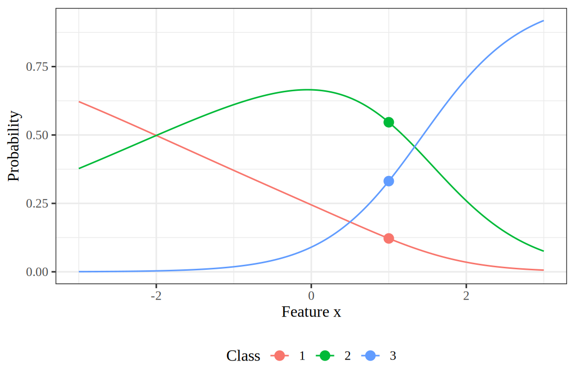
Figure 1
Line plot of three class probabilities against the feature x from minus 3 to 3. Class 1 starts near 0.6 and falls toward 0 as x grows. Class 2 rises to a peak near 0.67 at x about 0, then falls. Class 3 starts near 0 and rises toward 0.9. The three curves sum to 1 at every x. Points at x equal to 1 mark the probabilities 0.122, 0.547 and 0.331 computed in the example.
Show code
import numpy as np

b_mlr = np.array([[0.0, 1.0, -1.0], [0.0, 0.5, 2.0]])
x_mlr = np.array([1.0, 1.0])
linpred_mlr = b_mlr.T @ x_mlr
print(np.vstack([linpred_mlr, np.exp(linpred_mlr) / np.exp(linpred_mlr).sum()]).round(3))
[[0.    1.5   1.   ]
 [0.122 0.547 0.331]]
Show code
import pandas as pd
import plotnine as p9

x_grid = np.linspace(-3, 3, 200)
design = np.column_stack([np.ones_like(x_grid), x_grid])
grid_exp = np.exp(design @ b_mlr)
grid_prob = grid_exp / grid_exp.sum(axis=1, keepdims=True)
curves = pd.DataFrame({
    "x": np.tile(x_grid, 3),
    "class": np.repeat(["1", "2", "3"], 200),
    "probability": grid_prob.T.ravel(),
})
marked = pd.DataFrame({
    "x": 1.0,
    "class": ["1", "2", "3"],
    "probability": np.exp(linpred_mlr) / np.exp(linpred_mlr).sum(),
})
mlr_plot = (
    p9.ggplot(data=curves, mapping=p9.aes(x="x", y="probability", colour="class"))
    + p9.geom_line()
    + p9.geom_point(data=marked, size=3)
    + p9.labs(x="Feature x", y="Probability", colour="Class")
    + p9.theme_bw()
)
mlr_plot.show();
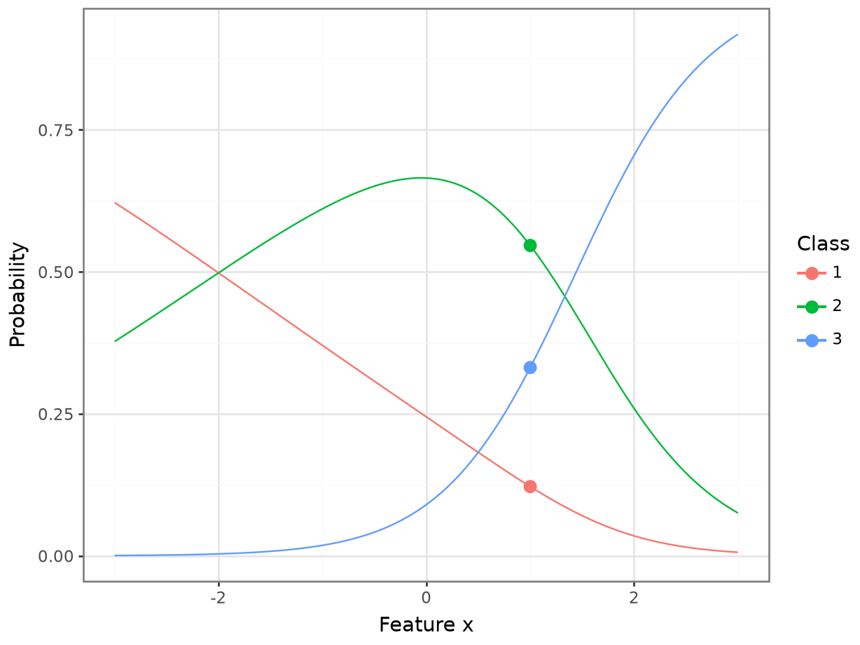
Figure 2
Line plot of three class probabilities against the feature x from minus 3 to 3. Class 1 starts near 0.6 and falls toward 0 as x grows. Class 2 rises to a peak near 0.67 at x about 0, then falls. Class 3 starts near 0 and rises toward 0.9. The three curves sum to 1 at every x. Points at x equal to 1 mark the probabilities 0.122, 0.547 and 0.331 computed in the example.

The linear predictors \(\tp{B}\vx\) are 0, 1.5 and 1, and their softmax gives the class probabilities 0.122, 0.547 and 0.331. Class 2 has the highest linear predictor, so it has the highest probability.

LemTheorem 1 (The two-class multinomial model is logistic regression)

Theorem 1 (The two-class multinomial model is logistic regression) In the multinomial model with \(C = 2\) and classes labeled \(0\) and \(1\),

\[ \condPr{\Outvar = 1}{\vx} = \sigmoidf{\dprod{\paren{B_1 - B_0}}{\vx}}, \]

so it is a logistic regression model with coefficient vector \(\vcoef = B_1 - B_0\).

Proof. Dividing the numerator and the denominator of the model by \(\e{\tp{B_1} \vx}\) gives

\[ \condPr{\Outvar = 1}{\vx} = \frac{1}{1 + \e{-\dprod{\paren{B_1 - B_0}}{\vx}}}, \]

which is the logistic function of \(\dprod{\paren{B_1 - B_0}}{\vx}\).

ExrExercise 5 (More than two classes (part 2))

Exercise 5 (More than two classes (part 2)) Use the setup of Exercise 4. By Theorem 1, the case \(C = 2\) is logistic regression. Here \(C\) is general.

Show that replacing every \(B_m\) by \(B_m + \v{c}\), for any fixed vector \(\v{c}\), leaves all \(C\) probabilities unchanged. How many free parameters does the model have? Give two ways to remove the excess, and state which one Solution 4 used.

Solution 5. Adding \(\v{c}\) to each \(B_k\) multiplies the numerator and every term of the denominator by the same factor \(\e{\tp{\v{c}}\vx}\), which cancels:

\[ \begin{aligned} \frac{\e{\tp{(B_m + \v{c})}\vx}}{\sum_k \e{\tp{(B_k + \v{c})}\vx}} &= \frac{\e{\tp{\v{c}}\vx + \tp{B_m}\vx}}{\sum_k \e{\tp{\v{c}}\vx + \tp{B_k}\vx}} && \text{(distribute the dot product over the sum)} \\ &= \frac{\e{\tp{\v{c}}\vx}\,\e{\tp{B_m}\vx}}{\sum_k \e{\tp{\v{c}}\vx}\,\e{\tp{B_k}\vx}} && \text{(exponential of a sum)} \\ &= \frac{\e{\tp{\v{c}}\vx}\,\e{\tp{B_m}\vx}}{\e{\tp{\v{c}}\vx}\sum_k \e{\tp{B_k}\vx}} && \text{(factor the common term out of the sum)} \\ &= \frac{\e{\tp{B_m}\vx}}{\sum_k \e{\tp{B_k}\vx}} && \text{(cancel the common factor $\e{\tp{\v{c}}\vx} > 0$)} \\ &= P(Y = m \mid \vx) && \text{(the model)}. \end{aligned} \]

The model is therefore overparameterized. With \(\vx \in \reals^{\ninputvars + 1}\), it has \(C(\ninputvars+1)\) parameters, but only \((C-1)(\ninputvars+1)\) of them are identified: adding a common vector \(\v{c}\) to all \(C\) columns moves \(B\) within a \((\ninputvars+1)\)-dimensional set of matrices on which the likelihood is constant. The Hessian of the log-likelihood is singular in those directions, so an unregularized Newton solver cannot invert it without a constraint.

Two standard ways to remove this non-identifiability are:

  • Designate a reference class: set \(B_1 = \vzero\) and interpret every other \(B_m\) relative to class \(1\). Solution 4 used this convention for \(C = 2\) by setting \(B_0 = \vzero\), so that \(\vcoef = B_1\).
  • Add a ridge penalty. Subtracting \(\tfrac{\regpar}{2}\sum_m \norm{B_m}^2\) from the log-likelihood, for some \(\regpar > 0\), makes the objective strictly concave, so it has at most one maximizer. Among the matrices \(B + \v{c}\tp{\boldsymbol{1}}\) that give the same probabilities, the penalty is smallest when the \(C\) columns sum to \(\vzero\), so the maximizer satisfies \(\sum_m B_m = \vzero\). Neural network classifiers typically retain all \(C\) columns and rely on weight decay or on first-order optimization, which does not invert the Hessian.

Retaining all \(C\) columns treats all classes symmetrically, uses the same gradient formula for every class, and stores the parameters in a single \((\ninputvars+1) \times C\) matrix, with \(\ninputvars+1\) redundant parameters.

The two approaches differ in what they do to the fitted probabilities. A reference class changes no fitted probability: it selects one matrix \(B\) among those that give the same probabilities, which is why different software packages can report different coefficients for the same fitted model. A ridge penalty also shrinks the coefficients toward \(\vzero\), so it changes the fitted probabilities, by less the smaller \(\regpar\) is.

3 Ordered classes

When the classes have a natural order, such as ratings from poor to excellent, the multinomial model discards that order. It also needs a separate coefficient vector for each class. Modeling the cumulative probabilities instead uses one coefficient vector and a threshold for each boundary between classes.

DefDefinition 3 (Ordinal logistic regression (cumulative logit model, proportional odds model))

Definition 3 (Ordinal logistic regression (cumulative logit model, proportional odds model)) For a label \(\Outvar\) with \(C\) ordered classes \(1 < \dots < C\) and a feature vector \(\vx\) with no entry for the intercept, an ordinal logistic regression model, also called a cumulative logit model or proportional odds model, has a coefficient vector \(\vcoef\) and thresholds \(\thresh_1 < \dots < \thresh_{C-1}\) that satisfy

\[ \logitf{\Prf{\Outvar \le m \given \vx}} = \thresh_m - \dprod{\vcoef}{\vx}, \qquad m = 1, \dots, C-1 \tag{3}\]

[6].

ExmExample 3 (Class probabilities from ordered thresholds)

Example 3 (Class probabilities from ordered thresholds) Let there be \(C = 3\) ordered classes, and one feature \(\predvar\). Let \(\thresh_1 = -1\), \(\thresh_2 = 1\) and \(\coef{\predvar} = 1\). Compute the class probabilities at \(\predvar = 1\).

Show code
ord_theta <- c(-1, 1)
ord_beta <- 1
ord_x <- 1
ord_cumulative <- plogis(ord_theta - ord_beta * ord_x)
ord_cumulative_full <- c(0, ord_cumulative, 1)
ord_prob <- diff(ord_cumulative_full)
ord_cumulative_top <- c(ord_cumulative, 1)
# nolint start: undesirable_function_linter. A two-row matrix.
rbind(cumulative = ord_cumulative_top, probability = ord_prob) |> round(3)
             [,1]  [,2] [,3]
cumulative  0.119 0.500  1.0
probability 0.119 0.381  0.5
Show code
# nolint end
Show code
import numpy as np
from scipy.special import expit

theta_ord = np.array([-1.0, 1.0])
beta_ord = 1.0
x_ord = 1.0
cumulative_ord = expit(theta_ord - beta_ord * x_ord)
cumulative_full_ord = np.concatenate([[0.0], cumulative_ord, [1.0]])
print(np.vstack([cumulative_full_ord[1:], np.diff(cumulative_full_ord)]).round(3))
[[0.119 0.5   1.   ]
 [0.119 0.381 0.5  ]]

The cumulative probabilities are \(0.119\), \(0.5\) and \(1\). The class probabilities are their consecutive differences: \(0.119\), \(0.381\) and \(0.5\). Changing a threshold moves one boundary between classes. Changing the coefficient moves both boundaries together.

ExrExercise 6 (Probabilities of ordered classes)

Exercise 6 (Probabilities of ordered classes) Use the model with \(C\) ordered classes. Write \(\Prf{\Outvar = m \given \vx}\) for \(m = 1, \dots, C\) using the sigmoid function.

Solution 6. The event \(\Outvar = m\) is \(\Outvar \le m\) without \(\Outvar \le m - 1\). Its probability is therefore the difference of two consecutive cumulative probabilities. Define \(\thresh_0 = -\infty\) and \(\thresh_C = \infty\), so that \(\sigmoidf{\thresh_0 - \dprod{\vcoef}{\vx}} = 0\) and \(\sigmoidf{\thresh_C - \dprod{\vcoef}{\vx}} = 1\). Then

\[ \Prf{\Outvar = m \given \vx} = \sigmoidf{\thresh_m - \dprod{\vcoef}{\vx}} - \sigmoidf{\thresh_{m-1} - \dprod{\vcoef}{\vx}}, \qquad m = 1, \dots, C. \]

The probabilities are nonnegative because the sigmoid function is increasing and \(\thresh_{m-1} < \thresh_m\).

ExrExercise 7 (Shifting the features (part 2))

Exercise 7 (Shifting the features (part 2)) Use the model. Take two feature vectors \(\vx\) and \(\vx'\). Compare the log-odds of \(\Outvar \le m\) at the two, for each \(m\).

Solution 7. The log-odds function is the inverse of the sigmoid function, so by Equation 3

\[ \logitf{\Prf{\Outvar \le m \given \vx}} = \thresh_m - \dprod{\vcoef}{\vx}. \]

Subtracting the same expression at \(\vx'\) gives

\[ \logitf{\Prf{\Outvar \le m \given \vx}} - \logitf{\Prf{\Outvar \le m \given \vx'}} = -\dprod{\vcoef}{\paren{\vx - \vx'}}, \]

which does not depend on \(m\). The odds of \(\Outvar \le m\) are multiplied by the same factor \(\e{-\dprod{\vcoef}{\paren{\vx - \vx'}}}\) for every \(m\). That shared factor is why the model is called the proportional odds model.

4 Comparing softmax probability vectors

ExrExercise 8 (Comparing softmax probability vectors)

Exercise 8 (Comparing softmax probability vectors) Sketch the probability mass function that the softmax function produces for each of these score vectors, showing only the relative heights of the three probabilities in each:

\[\vv_1 = \operatorname{softmax}\!\begin{pmatrix}0\\0\\0\end{pmatrix}, \quad \vv_2 = \operatorname{softmax}\!\begin{pmatrix}3\\3\\3\end{pmatrix}, \quad \vv_3 = \operatorname{softmax}\!\begin{pmatrix}0\\-1\\2\end{pmatrix}, \quad \vv_4 = \operatorname{softmax}\!\begin{pmatrix}2\\0\\0\end{pmatrix}.\]

Then state which two are identical, and why, without computing any exponentials.

Solution 8. The probability vectors \(\vv_1\) and \(\vv_2\) are equal.

Solution 5 showed that adding the same number, \(\tp{\v{c}}\vx\), to every score leaves the softmax unchanged. Every entry of \(\pt{3,3,3}\) is \(3\) more than the matching entry of \(\pt{0,0,0}\), so the two score vectors give the same probability vector.

Both \(\vv_1\) and \(\vv_2\) are uniform, with \(1/3\) in each coordinate (Figure 3). In \(\vv_3\), the third coordinate is the largest and the second is the smallest, close to \(0\). In \(\vv_4\), the first coordinate is the largest, and the second and third are equal and smaller.

Figure 3: The probability mass functions of the four softmax vectors. Vectors 1 and 2 give the same probabilities, one third each. Vector 3, from the scores \(\pt{0, -1, 2}\), puts most of its mass on the third class, and vector 4, from \(\pt{2, 0, 0}\), on the first.
ExrExercise 9 (Comparing softmax probability vectors (part 2))

Exercise 9 (Comparing softmax probability vectors (part 2)) Use the setup of Exercise 8.

Give all four to three decimal places.

Solution 9.

Table 1: The three values for each of four score vectors.
class 1 class 2 class 3
\(\vv_1\) \(0.333\) \(0.333\) \(0.333\)
\(\vv_2\) \(0.333\) \(0.333\) \(0.333\)
\(\vv_3\) \(0.114\) \(0.042\) \(0.844\)
\(\vv_4\) \(0.787\) \(0.107\) \(0.107\)
ExrExercise 10 (Comparing softmax probability vectors (part 3))

Exercise 10 (Comparing softmax probability vectors (part 3)) Use the setup of Exercise 8.

In \(\vv_3\), the largest score exceeds the smallest by \(3\). Give the ratio of the corresponding two probabilities, exactly, and state what determines it.

Solution 10. Write \(p_m = \operatorname{softmax}(\vz)_m\) and \(Z\) for the normalizer of Definition 1. The ratio of any two softmax probabilities is

\[ \begin{aligned} \frac{p_m}{p_k} &= \frac{\e{z_m}/Z}{\e{z_k}/Z} && \text{(definition of the softmax)} \\ &= \frac{\e{z_m}}{\e{z_k}} && \text{(the normalizer $Z$ cancels)} \\ &= \e{z_m - z_k} && \text{(quotient of exponentials)}. \end{aligned} \]

Here \(z_3 - z_2 = 2 - (-1) = 3\), so

\[ \begin{aligned} p_3/p_2 &= \e{3} \\ &= 20.09, \end{aligned} \]

which is the ratio of the unrounded probabilities of Solution 9, 20.09.

This ratio depends only on the difference \(z_m - z_k\), not on the individual values of \(z_m\) and \(z_k\), the number of classes, or the scores of the other classes. This property is the pairwise form of the shift invariance in Solution 8. Taking logarithms gives \(\log\paren{p_m / p_k} = z_m - z_k\): the difference between two class scores is the log of the ratio of their probabilities. With two classes, this log ratio is the log-odds of the log-odds exercise.

ExrExercise 11 (Comparing softmax probability vectors (part 4))

Exercise 11 (Comparing softmax probability vectors (part 4)) Use the setup of Exercise 8.

Raising the first score of \(\vv_4\) moves the output toward the indicator vector \((1, 0, 0)\). What must the scores approach for the softmax output to equal \((1, 0, 0)\), and how does this relate to the separation exercise?

Solution 11. No finite score vector produces \(\pt{1, 0, 0}\). Because \(\e{z_m} > 0\) for every finite \(z_m\), every softmax probability \(p_m\) is strictly positive. The softmax output approaches \(\pt{1, 0, 0}\) only in the limit as \(z_1 - z_2 \to +\infty\) and \(z_1 - z_3 \to +\infty\).

This behavior is the \(C\)-class version of the separation exercise. Suppose some coefficient matrix \(B\) gives every training observation a strictly larger score for its own class than for any other class, the multi-class version of linearly separable classes. Multiplying \(B\) by a growing positive number makes every score difference grow without bound, so every fitted probability of an observed class approaches \(1\), and the likelihood approaches \(1\). No finite \(B\) reaches likelihood \(1\), because every probability is less than \(1\), so the coefficients grow without bound and no finite maximum likelihood estimate exists. For \(C = 2\), the fact that every probability is in \((0, 1)\) reduces to the sigmoid properties exercise: \(\sigmoid(\logodds) \in (0,1)\) for all finite \(\logodds\).

5 Fitting the model

ExrExercise 12 (More than two classes (part 3))

Exercise 12 (More than two classes (part 3)) Use the setup of Exercise 4.

Derive \(\grad_{B_m}\,\ell\) for a dataset of \(\nobs\) observations, where \(\ell = \sum_i \log P(\Outvar = \outvar_i \mid \vx_i)\). Some references write a factor of \(1/\nobs\) in front of this gradient. Explain when that factor is correct and when it is a mistake.

Solution 12. Substitute the model into the log-likelihood:

\[ \begin{aligned} \ell &= \sum_i \log \frac{\e{\tp{B_{\outvar_i}}\vx_i}}{\sum_k \e{\tp{B_k}\vx_i}} && \text{(the model)} \\ &= \sum_i \sb{\log \e{\tp{B_{\outvar_i}}\vx_i} - \log\sum_k \e{\tp{B_k}\vx_i}} && \text{(log of a quotient)} \\ &= \sum_i \sb{\tp{B_{\outvar_i}}\vx_i - \log\sum_k \e{\tp{B_k}\vx_i}} && \text{(log of an exponential)}. \end{aligned} \]

The first term contributes \(\vx_i\) to \(\grad_{B_m}\) when \(y_i = m\) and \(\vzero\) otherwise, which equals \(\truthind(y_i = m)\,\vx_i\). In the second term, only the \(k = m\) summand depends on \(B_m\), so

\[ \begin{aligned} \grad_{B_m}\log\sum_k \e{\tp{B_k}\vx_i} &= \frac{1}{\sum_k \e{\tp{B_k}\vx_i}}\,\grad_{B_m}\sum_k \e{\tp{B_k}\vx_i} && \text{(chain rule for the logarithm)} \\ &= \frac{1}{\sum_k \e{\tp{B_k}\vx_i}}\,\grad_{B_m}\e{\tp{B_m}\vx_i} && \text{(only the $k = m$ summand depends on $B_m$)} \\ &= \frac{1}{\sum_k \e{\tp{B_k}\vx_i}}\,\e{\tp{B_m}\vx_i}\,\vx_i && \text{(chain rule for the exponential)} \\ &= P(Y = m \mid \vx_i)\,\vx_i && \text{(the model)}. \end{aligned} \]

Combining the two terms gives

\[\grad_{B_m}\,\ell = \sumin\sb{\truthind(y_i = m) - P(Y = m \mid \vx_i)}\vx_i,\]

which has the same form as the binary gradient: the residual times the feature vector, summed over observations.

Whether the factor of \(1/\nobs\) belongs depends on the objective. Multiplying \(\grad_{B_m}\,\ell\) by \(-1/\nobs\) gives the gradient of the mean cross-entropy, an empirical risk, and multiplying it by \(-1\) alone gives the gradient of the summed cross-entropy, the negative log-likelihood. So the factor is correct for the mean and a mistake for the sum or for \(\ell\) itself. Multiplying an objective by a nonzero constant does not change where its gradient vanishes, so the two conventions yield the same maximum likelihood estimate.

The factor of \(1/\nobs\) does change step sizes and curvature. Including \(1/\nobs\) in the gradient rescales the effective step size by \(1/\nobs\), as analyzed in the stochastic-gradient exercises of the gradient descent chapter, and it rescales the Hessian by \(1/\nobs\), so standard errors computed from the rescaled Hessian without accounting for \(\nobs\) would be off by a factor of \(\sqrt{\nobs}\).

LemTheorem 2 (Gradient of the multinomial log-likelihood)

Theorem 2 (Gradient of the multinomial log-likelihood) In the multinomial logistic regression model, the gradient of the log-likelihood \(\llik = \sum_i \log P(\Outvar = \outvar_i \mid \vx_i)\) with respect to the coefficient vector \(B_m\) of class \(m\) is

\[ \grad_{B_m}\,\llik =\sumin\sb{\truthind(\outvar_i = m) - P(\Outvar = m \mid \vx_i)}\vx_i. \]

Proof. By Solution 12.

ExmExample 4 (The gradient for one observation)

Example 4 (The gradient for one observation) Use the three coefficient vectors of Example 2 and a single observation with \(\vx = \pt{1, 1}\) and class \(3\). At \(x = 1\), the probabilities \(P(\Outvar = m \mid \vx)\) are 0.122, 0.547 and 0.331 for \(m = 1, 2, 3\).

By Theorem 2, the gradient for class \(m\) is the residual \(\truthind(\outvar = m) - P(\Outvar = m \mid \vx)\) times \(\vx\). The residuals are -0.122, -0.547 and 0.669, so \(\grad_{B_1}\,\llik = \pt{-0.122, -0.122}\), \(\grad_{B_2}\,\llik = \pt{-0.547, -0.547}\) and \(\grad_{B_3}\,\llik = \pt{0.669, 0.669}\). Only the observed class has a residual above zero, so a step up the gradient raises the probability of class \(3\) and lowers the others.

ExrExercise 13 (More than two classes (part 4))

Exercise 13 (More than two classes (part 4)) Use the setup of Exercise 4.

Check Exercise 12 against the gradient exercise, part 2 by specializing to \(C = 2\) under the convention you chose in Exercise 5.

Solution 13. For \(C = 2\) with class \(0\) fixed at \(B_0 = \vzero\) and \(B_1 = \vcoef\), Solution 4 gives \(P(\Outvar = 1\mid\vx_i) = \prob_i\), and \(\truthind(\outvar_i = 1) = \outvar_i\) because \(\outvar_i \in \{0,1\}\). The gradient from Solution 12 for \(m = 1\) then becomes

\[ \begin{aligned} \grad_{\vcoef}\,\ell &= \sum_i \paren{y_i - \prob_i}\vx_i && \text{(substitute $\prob_i$ and $\outvar_i$)} \\ &= \tp{\design(\mx)}\paren{\vy - \vprob} && \text{(the rows $\vx_i$ of $\design(\mx)$, weighted and summed)}. \end{aligned} \]

This gradient is minus the gradient of the cost in the gradient exercise, part 2, because maximizing \(\ell\) is the same as minimizing \(-\ell\).

Once \(B_0 = \vzero\) is fixed, the \(m = 0\) score equation is redundant: its residuals are minus the \(m = 1\) residuals, because the two fitted probabilities sum to \(1\) and the two class indicators sum to \(1\). This redundancy reflects the reduction from \(C(\ninputvars+1)\) parameters to \((C-1)(\ninputvars+1)\) identified parameters in Solution 5.

ExrExercise 14 (More than two classes (part 5))

Exercise 14 (More than two classes (part 5)) Use the setup of Exercise 4.

Setting Exercise 12 to zero gives \(C\) score equations. Assume that \(\vx\) has an intercept component. Interpret in words the intercept entry of the score equation for class \(m\), and compare it with the gradient exercise, part 5.

Solution 14. The intercept entry of \(\vx_i\) is \(1\), so the intercept entry of the \(m\)th score equation is

\[\sumin\truthind(y_i = m) = \sumin P(Y = m\mid\vx_i).\]

The left side is the observed count in class \(m\), and the right side is the sum of the fitted probabilities of class \(m\). So the fitted model matches the sample count of every class.

The gradient exercise, part 5 is the \(C = 2\) special case, where matching the count of class \(1\) also matches the count of class \(0\), because the two probabilities sum to \(1\). With \(C\) classes, summing the \(C\) intercept equations over \(m\) gives \(\nobs\) on both sides, so any \(C-1\) of them imply the last, and only \(C-1\) are linearly independent.

These equations make the fitted model match the class totals, not predict each observation accurately: a model can match every class total while assigning inaccurate probabilities to individual observations. An intercept-only model, which gives every observation the same probabilities, is an example.

ExrExercise 15 (More than two classes (part 6))

Exercise 15 (More than two classes (part 6)) Use the setup of Exercise 4.

Fit the intercept-only model to \(100\) observations, of which \(10\), \(30\) and \(60\) are in classes \(1\), \(2\) and \(3\). Give the fitted probabilities, and the coefficients under the convention of Exercise 5 with class \(1\) as the reference.

Solution 15. With only an intercept, every \(\vx_i = 1\), so the fitted probabilities \(p_m\) are constant across observations. Let \(\nobs_m\) be the number of observations in class \(m\). The score equation of Solution 14 is then \(\nobs_m = 100\,p_m\), so

\[\hat p_1 = 0.1, \qquad \hat p_2 = 0.3, \qquad \hat p_3 = 0.6,\]

which are the sample proportions.

Fixing class \(1\) as the reference class sets \(b_1 = 0\). By Solution 10, the ratio of two softmax probabilities depends only on the difference of their scores:

\[ \begin{aligned} \frac{p_m}{p_1} &= \e{b_m - b_1} && \text{(ratio of two softmax probabilities)} \\ &= \e{b_m} && \text{(reference class, $b_1 = 0$)}. \end{aligned} \]

Taking logarithms gives \(\hat b_m = \log\paren{\hat p_m / \hat p_1}\), so

\[ \begin{aligned} \hat b_2 &= \log\frac{0.3}{0.1} \\ &= \log 3 \\ &= 1.0986, \end{aligned} \qquad \begin{aligned} \hat b_3 &= \log\frac{0.6}{0.1} \\ &= \log 6 \\ &= 1.7918. \end{aligned} \]

As a check, the exponentials of the scores are \(\e{0} = 1\), \(\e{\log 3} = 3\) and \(\e{\log 6} = 6\), and

\[1 + 3 + 6 = 10,\]

so dividing the exponentials \(1, 3, 6\) by the normalizer \(10\) gives \(0.1, 0.3, 0.6\).

Each coefficient is the log of the ratio of its class’s probability to the reference class’s probability, so its value depends on the choice of reference class, as in the worked fit exercise, part 5. If class \(3\) is the reference class instead (\(b_3 = 0\)), the same fitted model has parameters \(\hat b_1 = \log\tfrac16\) and \(\hat b_2 = \log\tfrac12\), while all fitted probabilities are unchanged.

6 Large scores and weight penalties

ExrExercise 16 (A softmax with large scores)

Exercise 16 (A softmax with large scores) Consider four classes with the score vector \(\vz = \pt{23,\ -100,\ -15,\ 20}\).

Exponentiate each score, give the normalizer \(Z = \sum_k \e{z_k}\), and give the four probabilities \(\operatorname{softmax}(\vz)\), each to two significant figures.

Solution 16.

Show code
ls_z <- c(23, -100, -15, 20)
ls_exp <- exp(ls_z)
ls_norm <- sum(ls_exp)
ls_prob <- ls_exp / ls_norm
# nolint start: undesirable_function_linter. A matrix.
rbind(exponential = ls_exp, softmax = ls_prob) |> signif(3)
                [,1]     [,2]     [,3]     [,4]
exponential 9.74e+09 3.72e-44 3.06e-07 4.85e+08
softmax     9.53e-01 3.64e-54 2.99e-17 4.74e-02
Show code
# nolint end
import numpy as np

z_ls = np.array([23.0, -100.0, -15.0, 20.0])
exp_ls = np.exp(z_ls)
print(f"normalizer: {exp_ls.sum():.4g}\n{np.vstack([exp_ls, exp_ls / exp_ls.sum()])}")
normalizer: 1.023e+10
[[9.74480345e+09 3.72007598e-44 3.05902321e-07 4.85165195e+08]
 [9.52574127e-01 3.63644905e-54 2.99025668e-17 4.74258732e-02]]

Exponentiating gives \(9.74\times 10^{9}\), \(3.72\times 10^{-44}\), \(3.06\times 10^{-7}\) and \(4.85\times 10^{8}\). Only the first and the last are comparable in magnitude to the normalizer \(Z = 1.023\times 10^{10}\), so dividing each exponential by \(Z\) gives, to two significant figures,

\[\operatorname{softmax}(\vz) = \pt{\,0.95,\ 3.6\times 10^{-54},\ 3\times 10^{-17},\ 0.047\,} .\]

ExrExercise 17 (A softmax with large scores (part 2))

Exercise 17 (A softmax with large scores (part 2)) Use the setup of Exercise 16.

State what the softmax keeps of the scores’ ordering and what it keeps of their spacing, using the gap of \(3\) between the two leading scores and the gap of \(38\) between the leading score and the third. Explain how that relates to the name softmax.

Solution 17. The softmax keeps the ordering of the scores, because the exponential function is strictly increasing. It does not keep their spacing: by Solution 10, a difference between two scores becomes a ratio between their probabilities. The difference of \(3\) between the two leading scores becomes a factor of \(\e{3} \approx\) 20 between their probabilities, and the difference of \(38\) between the leading score and the third gives the third class a probability of \(3\times 10^{-17}\). The name “softmax” refers to this behavior: the softmax is a smooth approximation to the indicator vector of the largest score, and at this spacing it gives nearly all of the probability to the largest score.

ExrExercise 18 (A softmax with large scores (part 3))

Exercise 18 (A softmax with large scores (part 3)) Use the setup of Exercise 16.

In double-precision floating-point arithmetic, \(\e{z}\) overflows to infinity just below \(z = 710\). State what a direct implementation returns for the scores \(\vz + 700\), and use Exercise 5 to give an implementation that cannot overflow.

Solution 18. Adding \(700\) to every score gives the scores 723, 600, 685 and 720. The exponentials \(\e{723}\) and \(\e{720}\) exceed the overflow threshold, so they become infinity, and the normalizer becomes infinity with them. Direct evaluation then divides infinity by infinity for the first and last classes, returning NaN, and divides a finite number by infinity for the other two classes, returning \(0\). The exact probability vector equals the vector of Solution 16, because adding the same number to every score leaves every softmax probability unchanged, by Solution 5.

That shift invariance also prevents overflow. Before exponentiating, subtract the maximum score \(\max_k z_k\) from every entry. This shift leaves the probabilities unchanged and makes the largest exponential \(\e{0} = 1\), so no term can overflow, and because the normalizer is then at least \(1\), it cannot underflow to \(0\).

# nolint start: function_location_linter. Two helpers used only here.
softmax_direct <- function(z) {
  e <- exp(z)
  e / sum(e)
}
softmax_stable <- function(z) {
  e <- exp(z - max(z))
  e / sum(e)
}
# nolint end
ls_big <- ls_z + 700
ls_direct <- softmax_direct(ls_big)
ls_stable <- softmax_stable(ls_big)
# nolint start: undesirable_function_linter. A matrix.
rbind(direct = ls_direct, stable = ls_stable) |> signif(2)
       [,1]    [,2]  [,3]  [,4]
direct  NaN 0.0e+00 0e+00   NaN
stable 0.95 3.6e-54 3e-17 0.047
# nolint end
import numpy as np
from scipy.special import softmax

z_ls = np.array([23.0, -100.0, -15.0, 20.0]) + 700
with np.errstate(over="ignore", invalid="ignore"):
    direct_ls = np.exp(z_ls) / np.exp(z_ls).sum()
stable_ls = np.exp(z_ls - z_ls.max()) / np.exp(z_ls - z_ls.max()).sum()
print(f"direct: {direct_ls}\nstable: {stable_ls}\nscipy:  {softmax(z_ls)}")
direct: [nan  0.  0. nan]
stable: [9.52574127e-01 3.63644905e-54 2.99025668e-17 4.74258732e-02]
scipy:  [9.52574127e-01 3.63644905e-54 2.99025668e-17 4.74258732e-02]

SciPy’s scipy.special.softmax returns the same vector as the stable version, because it subtracts the maximum before exponentiating [7].

ExrExercise 19 (Penalizing the softmax weights)

Exercise 19 (Penalizing the softmax weights) Collect the class vectors as the columns of a \((\ninputvars+1) \times C\) matrix \(B\), with entries \(B_{rk}\) for row \(r\) and class \(k\). Index the rows by \(r = 0, 1, \dots, \ninputvars\), keeping \(i\) for observations. Row \(0\) holds the intercepts and rows \(1\) through \(\ninputvars\) the feature weights. Leave the intercepts out of the penalty, as the cross-entropy exercise, part 10b argued for the binary model, and maximize the penalized objective

\[J(B) = \llik(B) - \regpar\sumto{r}{\ninputvars}\sumto{k}{C} B_{rk}^2 .\]

Derive the gradient of \(J\) with respect to \(B_m\), using Exercise 12 for the gradient of \(\llik\).

Solution 19. The gradient of a difference is the difference of the gradients, so

\[\grad_{B_m} J(B) = \grad_{B_m}\,\llik(B) - \regpar\,\grad_{B_m}\sumto{r}{\ninputvars}\sumto{k}{C} B_{rk}^2 ,\]

and Solution 12 gives the first term. In the second gradient, only the terms from column \(m\) and rows \(r \ge 1\) depend on \(B_m\), and the derivative of \(B_{rm}^2\) with respect to \(B_{rm}\) is \(2 B_{rm}\), so

\[\grad_{B_m}\sumto{r}{\ninputvars}\sumto{k}{C} B_{rk}^2 = 2\tilde B_m, \qquad \tilde B_m = \pt{\,0,\; B_{1m},\; \dots,\; B_{\ninputvars m}\,},\]

where \(\tilde B_m\) is \(B_m\) with its intercept entry set to zero. Substituting both terms gives

\[\grad_{B_m} J(B) = \sumin\sb{\truthind(y_i = m) - P(Y = m \mid \vx_i)}\vx_i - 2\regpar\tilde B_m .\]

The penalty term pulls each non-intercept entry of \(B_m\) toward \(0\) in proportion to its magnitude, and it leaves the intercept entry unpenalized.

ExrExercise 20 (Penalizing the softmax weights (part 2))

Exercise 20 (Penalizing the softmax weights (part 2)) Use the setup of Exercise 19.

Exercise 5 showed that adding the same vector \(\v{c}\) to every column leaves the likelihood unchanged. State which of those shifts change the penalty, which representative of each equivalence class the penalized objective selects, and whether the remaining unpenalized direction in the intercept row affects the predicted probabilities.

Solution 20. Let the shift vector be \(\v{c} = \pt{c_0, c_1, \dots, c_{\ninputvars}}\). The penalty depends only on the feature rows \(r \ge 1\), where after the shift it equals \(\sum_{r \ge 1}\sum_k (B_{rk} + c_r)^2\). This sum depends on \(c_1, \dots, c_{\ninputvars}\), so the shifts that change any of \(c_1, \dots, c_{\ninputvars}\) change the penalty, although they give the same likelihood. Setting the derivative with respect to \(c_r\) to zero gives \(\sum_k (B_{rk} + c_r) = 0\). So the penalized objective selects the representative with the smallest penalty, in which each feature row sums to zero across the \(C\) classes.

Neither the likelihood nor the penalty depends on the intercept shift \(c_0\), so adding the same number to all \(C\) intercepts leaves the penalized objective unchanged. This shift does not change any predicted probability, but the objective is constant along it, so an optimizer that requires a unique maximizer must still fix one class intercept (for example, to \(0\)) or constrain the intercepts to sum to zero.

7 Videos

VideosWatch

Definitions on this page

References

[1]
G. James, D. Witten, T. Hastie, and R. Tibshirani, An introduction to statistical learning with applications in R, 2nd ed. Springer, 2021. Available: https://www.statlearning.com/
[2]
I. Goodfellow, Y. Bengio, and A. Courville, Deep learning. MIT Press, 2016. Available: https://www.deeplearningbook.org/
[3]
C. M. Bishop, Pattern recognition and machine learning. in Information science and statistics. New York: Springer, 2006.
[4]
GeeksforGeeks, “Softmax activation function in neural networks.” GeeksforGeeks, tutorial article, 2025. Available: https://www.geeksforgeeks.org/deep-learning/the-role-of-softmax-in-neural-networks-detailed-explanation-and-applications/
[5]
T. Hastie, R. Tibshirani, and J. Friedman, The elements of statistical learning: Data mining, inference, and prediction, 2nd ed. Springer, 2009. Available: https://hastie.su.domains/ElemStatLearn/
[6]
P. McCullagh, “Regression models for ordinal data,” Journal of the Royal Statistical Society: Series B (Methodological), vol. 42, no. 2, pp. 109–142, 1980, doi: 10.1111/j.2517-6161.1980.tb01109.x.
[7]
The SciPy Developers, “Source code of scipy.special.softmax, in scipy/special/_logsumexp.py.” SciPy version 1.18.1, 2026. Available: https://github.com/scipy/scipy/blob/v1.18.1/scipy/special/_logsumexp.py
[8]
T. Hastie, R. Tibshirani, and J. Taylor, “Statistical learning with python.” Stanford Online, lecture videos on YouTube, 2023. Available: https://www.youtube.com/playlist?list=PLoROMvodv4rPP6braWoRt5UCXYZ71GZIQ
[9]
B. Hutchinson, “DATA 471/571 (machine learning) and CSCI 481/581 (deep learning) video lectures.” Western Washington University. Accessed: Sep. 28, 2026. [Online]. Available: https://facultyweb.cs.wwu.edu/~hutchib2/video_lectures/data371/
[10]
J. Starmer, “Neural networks part 5: ArgMax and SoftMax.” StatQuest, video on YouTube, 2021. Available: https://www.youtube.com/watch?v=KpKog-L9veg
Back to top