Support Vector Machine Lab

Published

Last modified: 2026-11-19

Show code
# The Python chunks on this page import numpy, matplotlib and scikit-learn;
# reticulate provisions them.
py_packages <- c("numpy", "matplotlib", "scikit-learn")
library(reticulate) # nolint: undesirable_function_linter
py_require(py_packages)
1 The book’s Chapter 9 lab

This page holds the code lab for the Support Vector Machines chapter.

To work the lab without the solutions, download a stub with only the exercises:

Each solution shows the code in Python and in R with tidymodels.

Section 9.6 of the book [1] is the source of these exercises. The Python code follows the book’s Chapter 9 lab notebook, which fits models with SVC from scikit-learn [2]. The R code fits them with tidymodels, whose kernlab engine [3] plays the part of the e1071 package in the book’s R edition.

2 The support vector classifier

ExrExercise 1 (Lab: simulate two classes that overlap)

Exercise 1 (Lab: simulate two classes that overlap) Simulate \(50\) observations of two features, each standard normal. Label the first \(25\) observations \(-1\) and the last \(25\) observations \(+1\). Add \(1\) to both features of the observations labeled \(+1\).

TipHint

The random number functions draw normal values for a given array shape, and array tools build a vector of labels and add a number to selected rows.

Solution 1.

import numpy as np

rng = np.random.default_rng(1)
X_svc = rng.standard_normal((50, 2))
y_svc = np.array([-1] * 25 + [1] * 25)
X_svc[y_svc == 1] += 1
X_svc.shape
(50, 2)
library(tidymodels) # nolint: undesirable_function_linter

set.seed(1)
classes <- c(-1, 1)
labels <- rep(classes, each = 25)
shift <- as.numeric(labels == 1)
x1 <- rnorm(50)
x2 <- rnorm(50)
y <- factor(labels)
svc_data <- tibble(x1 = x1 + shift, x2 = x2 + shift, y = y)
dim(svc_data)
[1] 50  3
ExrExercise 2 (Lab: plot the simulated classes)

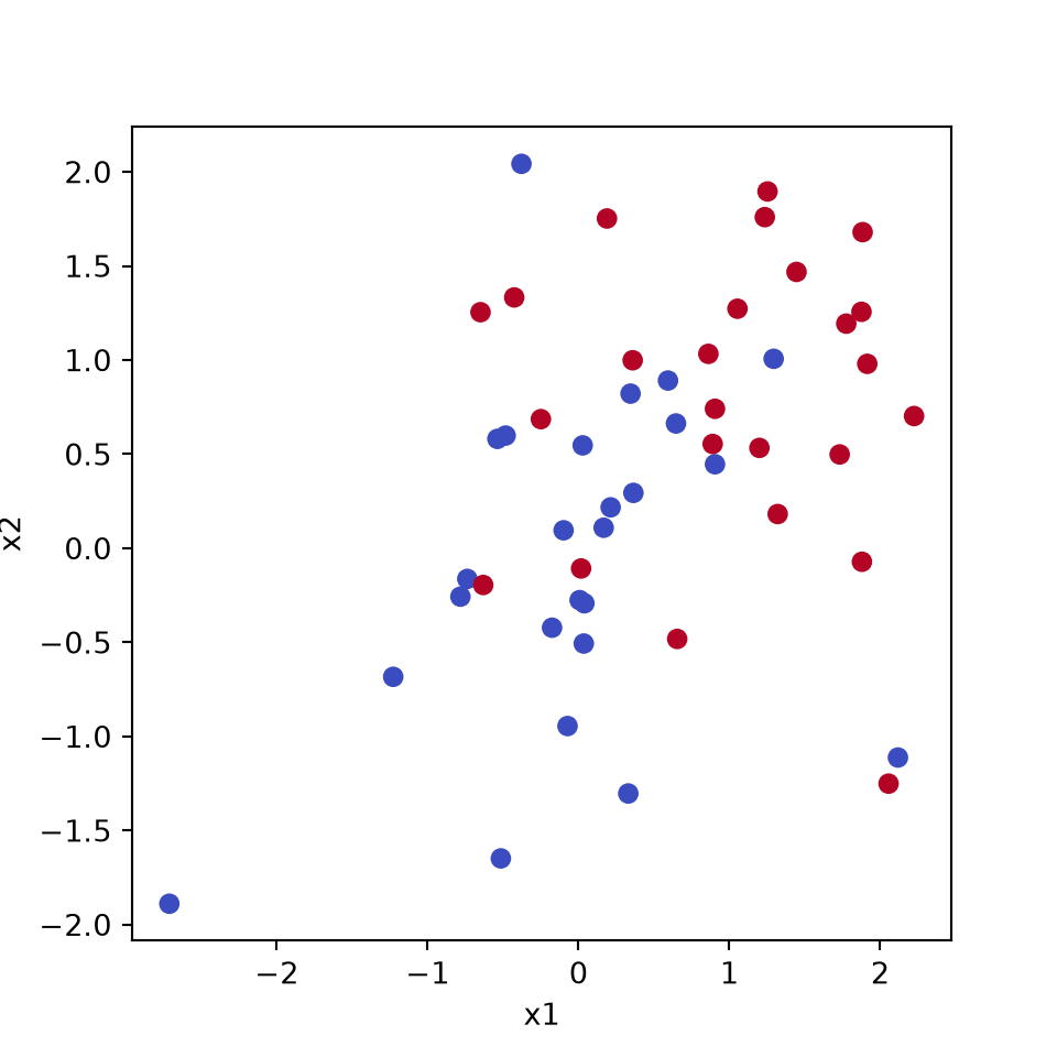
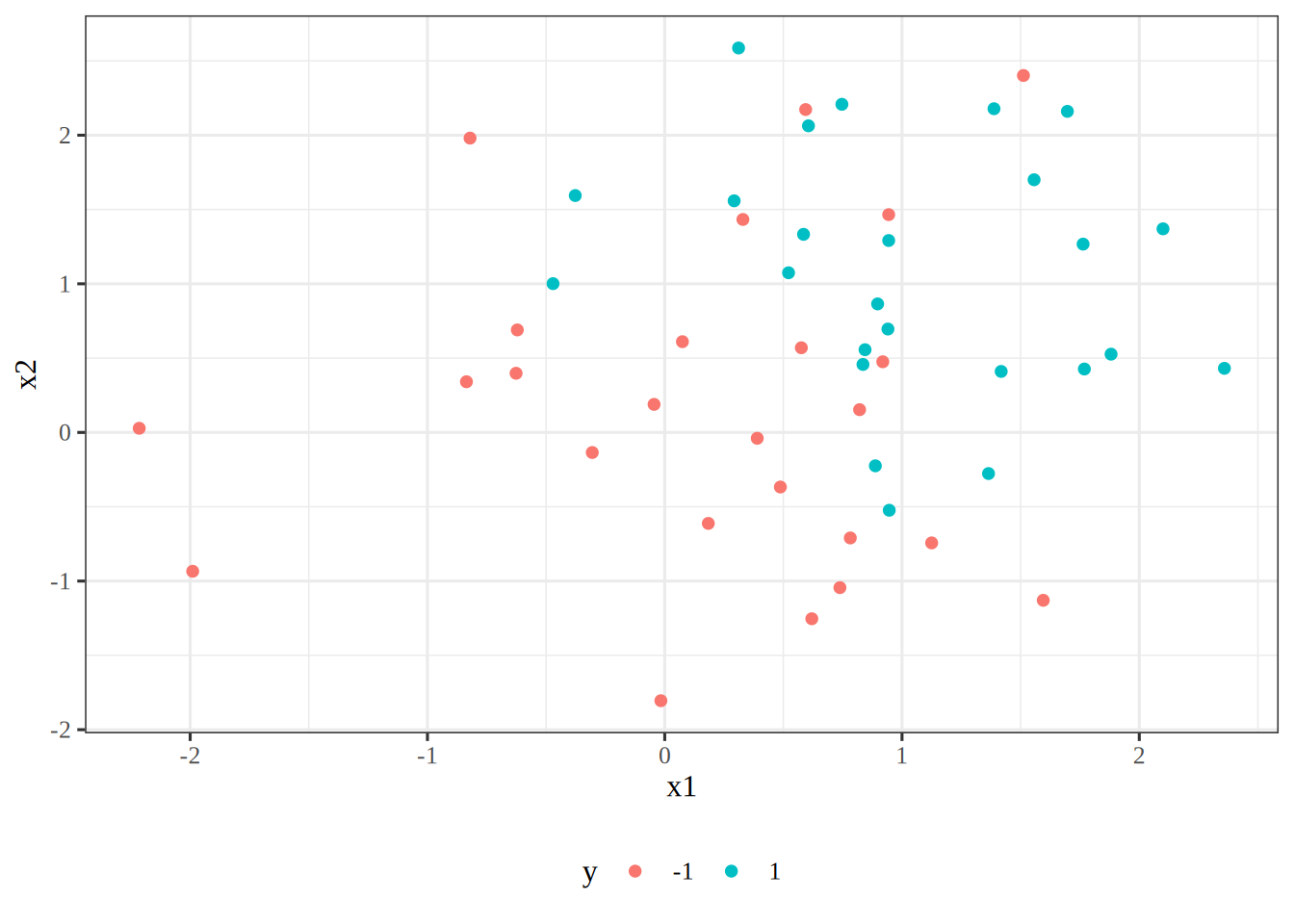
Exercise 2 (Lab: plot the simulated classes) Plot the two features of Solution 1 against each other. Color each observation by its label.

TipHint

A scatterplot takes one color for each observation, which you can choose from the label.

Solution 2.

Figure 1: The data plotted by x1 and x2, with the color showing the group of each dot.
import matplotlib.pyplot as plt

fig, ax = plt.subplots(figsize=(5, 5))
ax.scatter(X_svc[:, 0], X_svc[:, 1], c=y_svc, cmap="coolwarm");
ax.set_xlabel("x1");
ax.set_ylabel("x2");
plt.show()

svc_data |>
  ggplot(aes(x1, x2, color = y)) +
  geom_point()

In Figure 1, the two classes overlap. No line separates them. Even a linear classifier with an enormous cost makes 9 training errors in the R data and 13 in the Python data.

ExrExercise 3 (Lab: the mean of each feature in each class)

Exercise 3 (Lab: the mean of each feature in each class) Find the sample mean of each feature of Solution 1 within each label.

TipHint

Select the rows of one label with a comparison, then average each column of them. In R, group the table by label with group_by(), then summarize the columns.

Solution 3. This solution continues Solution 2.

svc_mean_neg_py = X_svc[y_svc == -1].mean(axis=0)
svc_mean_pos_py = X_svc[y_svc == 1].mean(axis=0)
svc_mean_neg_py.round(2), svc_mean_pos_py.round(2)
(array([-0.02, -0.05]), array([0.99, 0.79]))
svc_means_r <- svc_data |>
  group_by(y) |>
  summarise(across(c(x1, x2), mean))
svc_means_r
Show code
svc_means_gap <- svc_means_r |>
  summarise(across(c(x1, x2), diff))

The label \(+1\) has a larger mean in both features, by 0.86 in x1 and 0.9 in x2 in the R run. Both gaps are near \(1\), the shift added to the observations labeled \(+1\), but not equal to it, because each mean averages only \(25\) random draws. The two groups of observations overlap, because that gap is not large next to the standard deviation of \(1\) within each group.

ExrExercise 4 (Lab: fit a support vector classifier)

Exercise 4 (Lab: fit a support vector classifier) Fit a support vector classifier with a linear kernel and cost \(C = 10\) to the features and labels of Solution 1.

TipHint

Every estimator in scikit-learn is fit with .fit on a matrix of features and a vector of labels; the settings of a support vector classifier are its kernel function and its cost. In R, the svm_linear() specification of tidymodels is fit with fit().

Solution 4.

from sklearn.svm import SVC

svc_py = SVC(C=10, kernel="linear").fit(X_svc, y_svc)
svc_py
SVC(C=10, kernel='linear')
In a Jupyter environment, please rerun this cell to show the HTML representation or trust the notebook.
On GitHub, the HTML representation is unable to render, please try loading this page with nbviewer.org.
svc_spec <- svm_linear(mode = "classification", cost = 10)
svc_spec <- set_engine(svc_spec, "kernlab", scaled = FALSE)
svc_fit <- fit(svc_spec, y ~ x1 + x2, data = svc_data)
svc_fit
parsnip model object

Support Vector Machine object of class "ksvm" 

SV type: C-svc  (classification) 
 parameter : cost C = 10 

Linear (vanilla) kernel function. 

Number of Support Vectors : 28 

Objective Function Value : -263.7255 
Training error : 0.18 
Probability model included. 
ExrExercise 5 (Lab: count the support vectors)

Exercise 5 (Lab: count the support vectors) Find the number of support vectors of the fit in Solution 4.

TipHint

A fitted estimator stores what it learned in attributes whose names end in _; one of them holds the support vectors. In R, extract_fit_engine() returns the engine object. Then kernlab::nSV() counts its support vectors.

Solution 5.

svc_py_n_sv = int(svc_py.n_support_.sum())
svc_py_n_sv
29
svc_engine <- extract_fit_engine(svc_fit)
svc_r_n_sv <- kernlab::nSV(svc_engine)
svc_r_n_sv
[1] 28

The fit has 28 support vectors in the R run and 29 in the Python run. The two languages simulate different observations, so the counts differ.

ExrExercise 6 (Lab: find the training error)

Exercise 6 (Lab: find the training error) Find the training error of the fit in Solution 4, the proportion of the simulated observations it misclassifies.

TipHint

The .predict method returns a predicted label for each row, and the training error is the fraction that differ from the actual ones. In R, predict() on a tidymodels workflow plays the same role as .predict.

Solution 6.

svc_py_error = float((svc_py.predict(X_svc) != y_svc).mean())
svc_py_error
0.26
svc_pred <- predict(svc_fit, svc_data)
svc_r_error <- mean(svc_pred$.pred_class != svc_data$y)
svc_r_error
[1] 0.18

The overlapping classes force some errors. The training error is 0.18 in the R run and 0.26 in the Python run.

ExrExercise 7 (Lab: count the support vectors at a smaller cost)

Exercise 7 (Lab: count the support vectors at a smaller cost) Refit the classifier of Solution 4 with the cost \(C = 0.1\), and find the number of its support vectors.

TipHint

Refit as in Exercise 4 with one setting changed, then read off the support vectors as in Exercise 5.

Solution 7.

svc_py_small = SVC(C=0.1, kernel="linear").fit(X_svc, y_svc)
svc_py_n_sv_small = int(svc_py_small.n_support_.sum())
svc_py_n_sv_small
36
svc_spec_small <- update(svc_spec, cost = 0.1)
svc_fit_small <- fit(svc_spec_small, y ~ x1 + x2, data = svc_data)
svc_engine_small <- extract_fit_engine(svc_fit_small)
svc_r_n_sv_small <- kernlab::nSV(svc_engine_small)
svc_r_n_sv_small
[1] 38

The fit with \(C = 0.1\) has 38 support vectors in the R run and 36 in the Python run, more than the 28 and 29 at \(C = 10\). A smaller cost tolerates more slack, so the margin widens and more observations lie inside it or on it. This matches the monotonicity of the margin in \(C\).

ExrExercise 8 (Lab: choose the cost by cross-validation)

Exercise 8 (Lab: choose the cost by cross-validation) Choose the cost \(C\) from \(0.001\), \(0.01\), \(0.1\), \(1\), \(5\), \(10\) and \(100\) by five-fold cross-validation on the data of Solution 1, with accuracy as the score.

TipHint

A loop over the candidate values, with a cross-validation score of each, picks the best; the .score method of a classifier returns its accuracy. In R, tune_grid() with vfold_cv() tries the candidate values in tidymodels. Then select_best() picks one.

Solution 8.

from sklearn.model_selection import GridSearchCV, KFold

grid_py = GridSearchCV(
    SVC(kernel="linear"),
    {"C": [0.001, 0.01, 0.1, 1, 5, 10, 100]},
    cv=KFold(5, shuffle=True, random_state=0),
    scoring="accuracy",
).fit(X_svc, y_svc)

svc_py_best_c = float(grid_py.best_params_["C"])
svc_py_best_c
1.0
set.seed(2)
svc_folds <- vfold_cv(svc_data, v = 5)
# tune() marks the cost as the argument to tune
svc_tunable <- svm_linear(mode = "classification", cost = tune()) # nolint: nested_call_linter
svc_tunable <- set_engine(svc_tunable, "kernlab", scaled = FALSE)
svc_wf <- workflow()
svc_wf <- add_formula(svc_wf, y ~ x1 + x2)
svc_wf <- add_model(svc_wf, svc_tunable)
costs <- c(0.001, 0.01, 0.1, 1, 5, 10, 100)
cost_grid <- tibble(cost = costs)
accuracy_only <- metric_set(accuracy)
svc_tuned <- tune_grid(
  svc_wf,
  resamples = svc_folds,
  grid = cost_grid,
  metrics = accuracy_only
)
svc_best <- select_best(svc_tuned, metric = "accuracy")
svc_r_best_c <- svc_best$cost
svc_r_best_c
[1] 1

Several values of \(C\) can tie for the highest cross-validation accuracy, so the two libraries can choose different costs. The chosen cost is 1 in the R run and 1 in the Python run.

ExrExercise 9 (Lab: simulate a test set)

Exercise 9 (Lab: simulate a test set) Simulate \(20\) test observations the same way as the training data of Solution 1, \(10\) in each class.

TipHint

Draw the data with the random number functions exactly as in Exercise 1, with the new sizes.

Solution 9.

X_svc_test = rng.standard_normal((20, 2))
y_svc_test = np.array([-1] * 10 + [1] * 10)
X_svc_test[y_svc_test == 1] += 1
X_svc_test.shape
(20, 2)
labels_test <- rep(classes, each = 10)
shift_test <- as.numeric(labels_test == 1)
x1_test <- rnorm(20)
x2_test <- rnorm(20)
y_test <- factor(labels_test)
svc_test <- tibble(
  x1 = x1_test + shift_test,
  x2 = x2_test + shift_test,
  y = y_test
)
dim(svc_test)
[1] 20  3
ExrExercise 10 (Lab: find the test error of the tuned fit)

Exercise 10 (Lab: find the test error of the tuned fit) Predict the test observations of Solution 9 with the fit at the cost chosen in Solution 8, and find the test error.

TipHint

The .predict method returns a predicted label for each test row, and the test error is the fraction that differ from the actual ones. In R, predict() on a tidymodels workflow plays the same role as .predict.

Solution 10.

svc_py_test_pred = grid_py.predict(X_svc_test)
svc_py_test_error = float((svc_py_test_pred != y_svc_test).mean())
svc_py_test_error
0.3
svc_final <- finalize_workflow(svc_wf, svc_best)
svc_final <- fit(svc_final, svc_data)
svc_test_pred <- predict(svc_final, svc_test)
svc_r_test_error <- mean(svc_test_pred$.pred_class != svc_test$y)
svc_r_test_error
[1] 0.2

The test error is 0.2 in the R run and 0.3 in the Python run. Each is estimated from only \(20\) observations, so it varies a lot from one simulated sample to the next.

3 The radial kernel

ExrExercise 11 (Lab: simulate two classes with a nonlinear boundary)

Exercise 11 (Lab: simulate two classes with a nonlinear boundary) Simulate \(200\) observations of two features, each standard normal. Add \(2\) to both features of the first \(100\) observations, and subtract \(2\) from both features of the next \(50\). Label the first \(150\) observations \(1\) and the last \(50\) observations \(2\).

TipHint

Build the data with the random number functions and the array tools used in Exercise 1; shifting a block of rows is a slice plus a number.

Solution 11.

rng_rbf = np.random.default_rng(3)
X_rbf = rng_rbf.standard_normal((200, 2))
X_rbf[:100] += 2
X_rbf[100:150] -= 2
y_rbf = np.array([1] * 150 + [2] * 50)
X_rbf.shape
(200, 2)
set.seed(3)
shifts <- c(2, -2, 0)
shift_sizes <- c(100, 50, 50)
shift_rbf <- rep(shifts, times = shift_sizes)
x1_rbf <- rnorm(200)
x2_rbf <- rnorm(200)
label_values <- c(1, 2)
label_sizes <- c(150, 50)
labels_rbf <- rep(label_values, times = label_sizes)
y_rbf <- factor(labels_rbf)
rbf_data <- tibble(x1 = x1_rbf + shift_rbf, x2 = x2_rbf + shift_rbf, y = y_rbf)
dim(rbf_data)
[1] 200   3
ExrExercise 12 (Lab: fit a radial kernel and find its training error)

Exercise 12 (Lab: fit a radial kernel and find its training error) Fit a classifier with a radial kernel function, \(\gamma = 1\) and \(C = 1\), to the data of Solution 11, and find its training error.

TipHint

Every estimator in scikit-learn is fit with .fit; here the kernel function is radial, and \(\gamma\) and the cost are its settings. In R, the svm_rbf() specification of tidymodels is fit with fit().

Solution 12.

rbf_py = SVC(C=1, kernel="rbf", gamma=1).fit(X_rbf, y_rbf)
rbf_py_error = float((rbf_py.predict(X_rbf) != y_rbf).mean())
rbf_py_error
0.07
rbf_spec <- svm_rbf(mode = "classification", cost = 1, rbf_sigma = 1)
rbf_spec <- set_engine(rbf_spec, "kernlab", scaled = FALSE)
rbf_fit <- fit(rbf_spec, y ~ x1 + x2, data = rbf_data)
rbf_pred <- predict(rbf_fit, rbf_data)
rbf_r_error <- mean(rbf_pred$.pred_class != rbf_data$y)
rbf_r_error
[1] 0.085

The training error is 0.09 in the R run and 0.07 in the Python run. The radial kernel can bend the decision boundary around the middle class. The argument rbf_sigma of kernlab is the \(\gamma\) of the exercise.

4 ROC curves

ExrExercise 13 (Lab: find the area under the ROC curve)

Exercise 13 (Lab: find the area under the ROC curve) Find the area under the receiver operating characteristic curve of the radial-kernel fit of Solution 12 on its training data, scoring class \(2\) against class \(1\).

TipHint

The metrics functions of scikit-learn take the actual labels and a score for each row, which is the decision function of the fit.

Solution 13.

from sklearn.metrics import roc_auc_score

rbf_py_scores = rbf_py.decision_function(X_rbf)
rbf_py_auc = float(roc_auc_score(y_rbf == 2, rbf_py_scores))
rbf_py_auc
0.9781333333333333
rbf_probs <- predict(rbf_fit, rbf_data, type = "prob")
rbf_scored <- bind_cols(rbf_data, rbf_probs)
rbf_r_auc <- roc_auc(rbf_scored, truth = y, .pred_2, event_level = "second")
rbf_r_auc$.estimate
[1] 0.9496

The area is 0.95 in the R run and 0.98 in the Python run. A value near \(1\) says the fit scores nearly every observation of class \(2\) above every observation of class \(1\).

5 More than two classes

ExrExercise 14 (Lab: add a third class)

Exercise 14 (Lab: add a third class) Append \(50\) observations of two features, each standard normal, to the data of Solution 11. Add \(2\) to the second feature of the new observations, and label them \(0\).

TipHint

Stack rows of new observations under the old ones, and build the new labels with the array tools.

Solution 14.

X_new = rng_rbf.standard_normal((50, 2))
X_new[:, 1] += 2
X_multi = np.vstack([X_rbf, X_new])
y_multi = np.concatenate([y_rbf, np.zeros(50, dtype=int)])
X_multi.shape
(250, 2)
x1_new <- rnorm(50)
x2_new <- rnorm(50)
y_new <- factor(0)
new_data <- tibble(x1 = x1_new, x2 = x2_new + 2, y = y_new)
multi_data <- bind_rows(rbf_data, new_data)
dim(multi_data)
[1] 250   3
ExrExercise 15 (Lab: fit three classes and find the training error)

Exercise 15 (Lab: fit three classes and find the training error) Fit a classifier with a radial kernel function, \(\gamma = 1\) and \(C = 10\), to the data of Solution 14, and find its training error.

TipHint

Every estimator in scikit-learn is fit with .fit, and the training error is the fraction of predicted labels that differ from the actual ones; the number of classes does not change the call. In R, the svm_rbf() specification of tidymodels is fit with fit().

Solution 15.

multi_py = SVC(C=10, kernel="rbf", gamma=1).fit(X_multi, y_multi)
multi_py_error = float((multi_py.predict(X_multi) != y_multi).mean())
multi_py_error
0.14
multi_spec <- svm_rbf(mode = "classification", cost = 10, rbf_sigma = 1)
multi_spec <- set_engine(multi_spec, "kernlab", scaled = FALSE)
multi_fit <- fit(multi_spec, y ~ x1 + x2, data = multi_data)
multi_pred <- predict(multi_fit, multi_data)
multi_r_error <- mean(multi_pred$.pred_class != multi_data$y)
multi_r_error
[1] 0.132

The training error is 0.13 in the R run and 0.14 in the Python run. Both libraries fit the three classes with the one-versus-one approach: they fit a classifier to each pair of classes and take a vote.

References

[1]
G. James, D. Witten, T. Hastie, R. Tibshirani, and J. Taylor, An introduction to statistical learning: With applications in Python. Springer, 2023. doi: 10.1007/978-3-031-38747-0.
[2]
F. Pedregosa et al., “Scikit-learn: Machine learning in Python,” Journal of Machine Learning Research, vol. 12, pp. 2825–2830, 2011, Available: https://jmlr.org/papers/v12/pedregosa11a.html
[3]
A. Karatzoglou, A. Smola, K. Hornik, and A. Zeileis, “kernlab – an S4 package for kernel methods in R,” Journal of Statistical Software, vol. 11, no. 9, pp. 1–20, 2004, doi: 10.18637/jss.v011.i09.
Back to top