Interactions, Inference and Diagnostics

Published

Last modified: 2026-11-19

Show code
# The Python chunks import numpy, pandas, matplotlib, scipy and statsmodels;
# reticulate provisions them.
library(reticulate) # nolint: undesirable_function_linter
py_packages <- c("numpy", "pandas", "matplotlib", "scipy", "statsmodels")
py_require(py_packages)
# A positive number in scientific notation, for display math: 2.4\times10^{2}.
sci <- function(v) { # nolint: function_location_linter
  e <- v |> log10() |> floor()
  m <- signif(v / 10^e, 2)
  carry <- m >= 10
  if (carry) {
    m <- m / 10
    e <- e + 1
  }
  sprintf("%.1f\\times10^{%d}", m, e)
}

This material was part of the Auto lab page, which now keeps only the lab exercises. The sections follow [1, Ch. 3].

1 Fitted models on the Auto data

Every lab and example below reports 95% confidence intervals. These helpers are defined once, here, so no page depends on another page’s code. Each takes all its inputs as arguments.

Show code
import numpy as np


def bootstrap_corr_ci(a, b, B=20000, seed=571):
    """95% percentile interval for the correlation of a and b.

    Resamples the cases with replacement B times,
    which mimics drawing new cases from the same population,
    and recomputes the correlation each time.
    """
    rng = np.random.default_rng(seed)
    a, b = np.asarray(a, float), np.asarray(b, float)
    corr = np.empty(B)
    for i in range(B):
        rows = rng.integers(0, len(a), len(a))
        corr[i] = np.corrcoef(a[rows], b[rows])[0, 1]
    return np.quantile(corr, [0.025, 0.975])


def bootstrap_vif_ci(features, B=20000, seed=571):
    """95% percentile interval for each feature's VIF.

    The VIF of feature j is the jth diagonal entry
    of the inverse of the features' correlation matrix,
    which gives the same value as 1 / (1 - R^2) without a regression per feature.
    """
    rng = np.random.default_rng(seed)
    F = np.asarray(features, float)
    vifs = np.empty((B, F.shape[1]))
    for b in range(B):
        rows = rng.integers(0, len(F), len(F))
        vifs[b] = np.diag(np.linalg.inv(np.corrcoef(F[rows], rowvar=False)))
    return np.quantile(vifs, [0.025, 0.975], axis=0)
Show code
# Formats an interval's endpoints for the prose
ci_text <- function(bounds, digits) {
  sprintf("%.*f to %.*f", digits, bounds[[1]], digits, bounds[[2]])
}

# 95% percentile interval for R^2 from resampled cars.
# Resampling rows with replacement mimics
# drawing a new set of cars from the same population.
# The refits use lm.fit directly, because 2,000 workflow fits would be slow.
boot_r2_ci <- function(formula, data, n_boot = 2000) {
  set.seed(571)
  design <- model.matrix(formula, data)
  y <- model.response(model.frame(formula, data))
  r2 <- vapply(seq_len(n_boot), \(b) {
    rows <- sample(nrow(design), replace = TRUE)
    sse <- sum(lm.fit(design[rows, ], y[rows])$residuals^2)
    1 - sse / sum((y[rows] - mean(y[rows]))^2)
  }, numeric(1))
  unname(quantile(r2, c(0.025, 0.975)))
}

# 95% percentile interval for the correlation of a and b
boot_cor_ci <- function(a, b, n_boot = 20000) {
  set.seed(571)
  corr <- vapply(seq_len(n_boot), \(i) {
    rows <- sample(length(a), replace = TRUE)
    cor(a[rows], b[rows])
  }, numeric(1))
  unname(quantile(corr, c(0.025, 0.975)))
}

# 95% percentile interval for each feature's VIF.
# The VIF of feature j is the jth diagonal entry
# of the inverse of the features' correlation matrix,
# which gives the same value as 1 / (1 - R^2) without a regression per feature.
boot_vif_ci <- function(features, n_boot = 20000) {
  set.seed(571)
  vifs <- vapply(seq_len(n_boot), \(b) {
    resample <- features[sample(nrow(features), replace = TRUE), ]
    diag(solve(cor(resample)))
  }, numeric(ncol(features)))
  apply(vifs, 1, quantile, probs = c(0.025, 0.975))
}

# The 95% interval for a linear combination w'beta
# of a fitted model's coefficients:
# the estimate plus or minus a t quantile times its standard error,
# from the coefficients' covariance matrix
lincomb_ci <- function(model, w) {
  estimate <- sum(w * coef(model))
  half <- qt(0.975, df.residual(model)) * sqrt(drop(t(w) %*% vcov(model) %*% w))
  c(estimate = estimate, lower = estimate - half, upper = estimate + half)
}

The examples on this page use four least squares fits to the Auto data [2], each of a car’s miles per gallon (mpg) on some of its features:

  • the one-feature fit, on horsepower;
  • the two-feature fit, on horsepower and weight;
  • the quadratic fit, on horsepower and its square;
  • the origin fit, on weight and indicators for European and Japanese cars.

The Auto lab makes the same fits step by step.

Show code
import matplotlib.pyplot as plt
import numpy as np
import pandas as pd
import statsmodels.api as sm
from scipy import stats

# ISLP's load_data("Auto") reads this same file.
Auto = pd.read_csv("data/auto.csv")
mpg = Auto["mpg"]
y = mpg.to_numpy()
horsepower = Auto["horsepower"].to_numpy(float)
weight = Auto["weight"].to_numpy(float)
n = len(y)
origin = Auto["origin"].to_numpy()
european = (origin == 2).astype(float)
japanese = (origin == 3).astype(float)
place = Auto["origin"].map({1: "American", 2: "European", 3: "Japanese"})
origin_columns = pd.get_dummies(place, drop_first=True, dtype=float)
def fit(columns):
    Phi = np.column_stack([np.ones(n)] + columns)
    beta_hat = np.linalg.lstsq(Phi, y, rcond=None)[0]
    return beta_hat, Phi

def mean_squared_error(beta_hat, Phi):
    return np.mean((Phi @ beta_hat - y) ** 2)

def rmse(beta_hat, Phi):
    return np.sqrt(mean_squared_error(beta_hat, Phi))

def r_squared(beta_hat, Phi):
    sst = np.sum((y - y.mean()) ** 2)
    return 1 - mean_squared_error(beta_hat, Phi) * n / sst

def ols_summary(beta_hat, Phi, y_obs=y):
    """Residual degrees of freedom, the estimated noise variance, and (Phi'Phi)^{-1}."""
    df = len(y_obs) - Phi.shape[1]
    sigma2 = np.sum((y_obs - Phi @ beta_hat) ** 2) / df
    # The pseudoinverse gives (Phi'Phi)^{-1} without forming Phi'Phi,
    # which is badly conditioned for high-degree polynomials
    pinv = np.linalg.pinv(Phi)
    return df, sigma2, pinv @ pinv.T

def coef_ci(beta_hat, Phi):
    """95% interval for each coefficient: the estimate plus or minus a t quantile times its standard error."""
    df, sigma2, PtP_inv = ols_summary(beta_hat, Phi)
    half = stats.t.ppf(0.975, df) * np.sqrt(sigma2 * np.diag(PtP_inv))
    return np.column_stack([beta_hat - half, beta_hat + half])

def contrast_ci(beta_hat, Phi, c):
    """95% interval for the linear combination c'beta of the coefficients."""
    df, sigma2, PtP_inv = ols_summary(beta_hat, Phi)
    half = stats.t.ppf(0.975, df) * np.sqrt(sigma2 * c @ PtP_inv @ c)
    return c @ beta_hat - half, c @ beta_hat + half

def mean_ci(beta_hat, Phi, Phi_new, prediction=False, y_obs=y):
    """95% interval at the rows of Phi_new: for the mean response, or with prediction=True for one new response."""
    df, sigma2, PtP_inv = ols_summary(beta_hat, Phi, y_obs)
    # The variance of the fitted value, plus the noise of one new response for a prediction interval
    variance = sigma2 * (np.sum((Phi_new @ PtP_inv) * Phi_new, axis=1) + prediction)
    half = stats.t.ppf(0.975, df) * np.sqrt(variance)
    fitted_new = Phi_new @ beta_hat
    return fitted_new - half, fitted_new + half

def bootstrap_r2_ci(Phi, B=2000, seed=571):
    """95% percentile interval for R^2 from B resamples of the cars, refitted each time."""
    rng = np.random.default_rng(seed)
    r2 = np.empty(B)
    for b in range(B):
        rows = rng.integers(0, n, n)
        beta_b = np.linalg.lstsq(Phi[rows], y[rows], rcond=None)[0]
        sse = np.sum((y[rows] - Phi[rows] @ beta_b) ** 2)
        r2[b] = 1 - sse / np.sum((y[rows] - y[rows].mean()) ** 2)
    return np.quantile(r2, [0.025, 0.975])
Show code
beta_simple, Phi_simple = fit([horsepower])
beta_multiple, Phi_multiple = fit([horsepower, weight])
beta_quadratic, Phi_quadratic = fit([horsepower, horsepower ** 2])
beta_origin_weight, Phi_origin_weight = fit([weight, european, japanese])
fits = {
    "one-feature": beta_simple,
    "two-feature": beta_multiple,
    "quadratic": beta_quadratic,
    "origin": beta_origin_weight,
}
for name, beta in fits.items():
    print(f"{name}: {np.round(beta, 4)}")
one-feature: [39.9359 -0.1578]
two-feature: [ 4.56402e+01 -4.73000e-02 -5.80000e-03]
quadratic: [ 5.69001e+01 -4.66200e-01  1.20000e-03]
origin: [ 4.37322e+01 -7.00000e-03  9.70900e-01  2.32710e+00]
Show code
library(tidymodels) # nolint: undesirable_function_linter

auto <- readr::read_csv("data/auto.csv", show_col_types = FALSE)
lm_spec <- linear_reg() |> set_engine("lm")
fit_simple <- lm(mpg ~ horsepower, data = auto)
fit_multiple <- lm(mpg ~ horsepower + weight, data = auto)
fit_quadratic <- lm(mpg ~ horsepower + I(horsepower^2), data = auto)
fit_origin_weight <- lm(mpg ~ weight + factor(origin), data = auto)
fits <- list(
  one_feature = fit_simple,
  two_feature = fit_multiple,
  quadratic = fit_quadratic,
  origin = fit_origin_weight
)
fits |> map(coef)
$one_feature
(Intercept)  horsepower 
 39.9358610  -0.1578447 

$two_feature
 (Intercept)   horsepower       weight 
45.640210840 -0.047302863 -0.005794157 

$quadratic
    (Intercept)      horsepower I(horsepower^2) 
   56.900099702    -0.466189630     0.001230536 

$origin
    (Intercept)          weight factor(origin)2 factor(origin)3 
   43.732236152    -0.007027083     0.970905585     2.327149903 

2 Interaction terms

ExrExercise 1 (Does the horsepower slope depend on weight?)

Exercise 1 (Does the horsepower slope depend on weight?) In the two-feature fit, how much does the predicted mpg change per extra horsepower for a light car (\(2000\) pounds), and for a heavy car (\(4000\) pounds)?

Solution 1. The fitted model is \(\hat{y} = \hintcoef + \hcoef{1} \, \text{hp} + \hcoef{2} \, w\), where \(\text{hp}\) is horsepower and \(w\) is weight. Differentiating in \(\text{hp}\) gives \(\hcoef{1}\), which does not involve \(w\). So the change is -0.047 miles per gallon per horsepower for the light car and for the heavy car alike.

The same holds for every pair of features in a model that is a sum of one-feature terms: the effect of one feature on the prediction is the same at every value of the others. James et al. [1, Sec. 3.3.2], p. 94 calls this the additive assumption. To let the horsepower slope change with weight, the design matrix needs a column that combines the two features.

DatasetDataset 1: The advertising and sales (Advertising) data
Dataset 1: The advertising and sales (Advertising) data

Unit sales in 200 markets, with the advertising budget in each market, make up the Advertising data [1, Sec. 2.1]. The data are in data/advertising.csv, one row per market. The file is a copy of the Advertising data from the book’s website, statlearning.com. The columns are:

  • sales: the units sold, in thousands.
  • TV: the television advertising budget, in thousands of dollars.
  • radio: the radio advertising budget, in thousands of dollars.
  • newspaper: the newspaper advertising budget, in thousands of dollars.
DefDefinition 1 (Interaction term (product term, cross term))

Definition 1 (Interaction term (product term, cross term)) An interaction term (also called a product term or a cross term) between two features \(x_1\) and \(x_2\) is their product \(x_1 x_2\), used as an extra column of the design matrix [3]. It is a basis function of two inputs. With an interaction term, the feature map is \(\phi(\vx) = \tp{[1, x_1, x_2, x_1 x_2]}\), and the model is

\[ \modmemf{\vx} = \intcoef + \coef{1} x_1 + \coef{2} x_2 + \coef{3} x_1 x_2. \]

The slope of \(\modmem\) in \(x_1\), with \(x_2\) held fixed, is

\[ \frac{\partial \modmem}{\partial x_1} = \coef{1} + \coef{3} x_2, \]

so it changes with \(x_2\). In the same way, the slope in \(x_2\) is \(\coef{2} + \coef{3} x_1\). If \(\coef{3} = 0\), the model is additive, as in Solution 1.

Note 1: Other names for interactions

Marketing calls an interaction a synergy effect [1, Sec. 3.3.2], p. 95, and epidemiology calls it effect modification. These notes say interaction.

In R’s model formulas, x1:x2 is the product column alone, and x1 * x2 is short for x1 + x2 + x1:x2.

ExmExample 1 (Television and radio advertising)

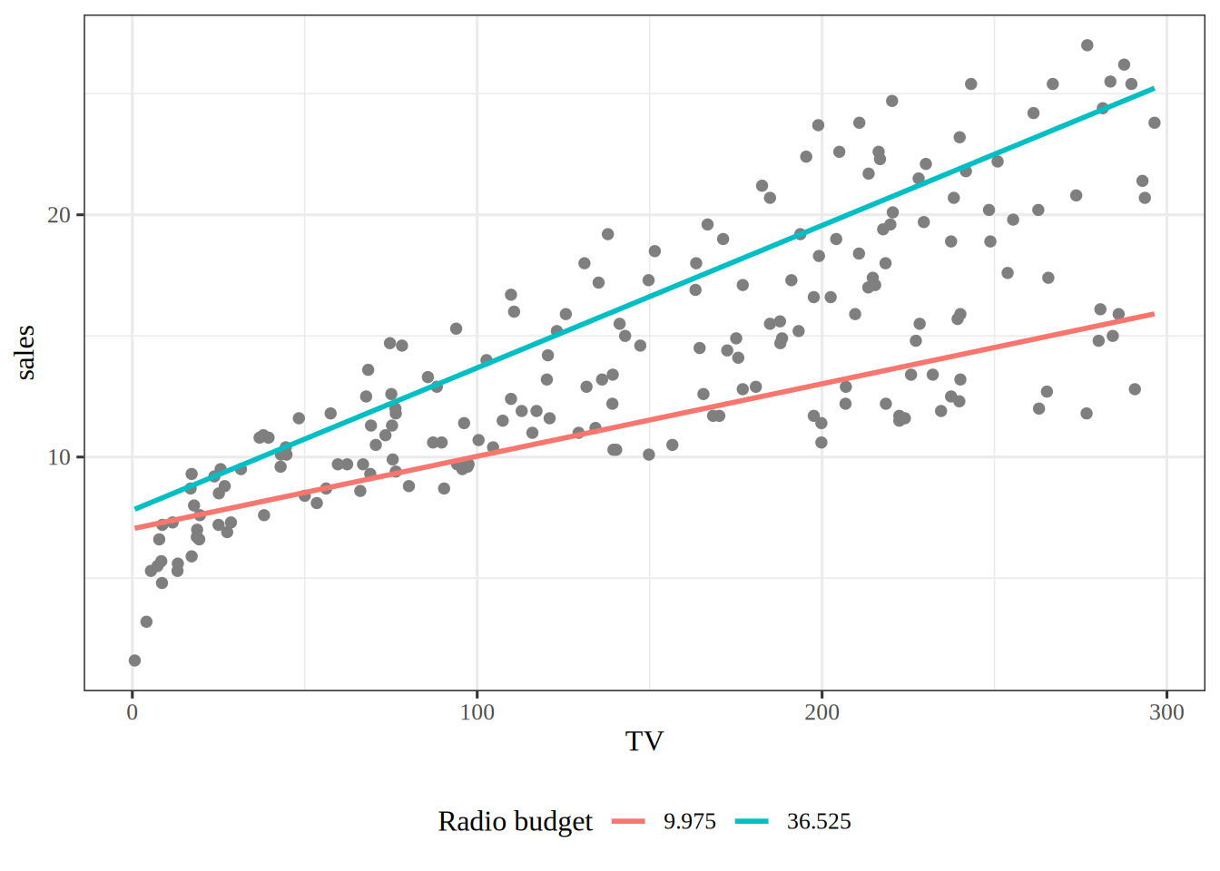
Example 1 (Television and radio advertising) In the Advertising data (Dataset 1), television advertising may sell more when radio advertising is also high. Fit sales on TV, radio and their interaction:

advertising = pd.read_csv("data/advertising.csv")
tv = advertising["TV"].to_numpy(float)
radio = advertising["radio"].to_numpy(float)
sales = advertising["sales"].to_numpy(float)
ones = np.ones(len(sales))

Phi_tv_radio = np.column_stack([ones, tv, radio, tv * radio])
beta_tv_radio = np.linalg.lstsq(Phi_tv_radio, sales, rcond=None)[0]
coef_names = ["intercept", "TV", "radio", "TV:radio"]
pd.Series(beta_tv_radio, index=coef_names).round(4)
intercept    6.7502
TV           0.0191
radio        0.0289
TV:radio     0.0011
dtype: float64
advertising <- readr::read_csv("data/advertising.csv", show_col_types = FALSE)
fit_tv_radio <- lm(sales ~ TV * radio, data = advertising)
fit_additive <- lm(sales ~ TV + radio, data = advertising)
parameters::parameters(fit_tv_radio) |>
  parameters::print_md(digits = 4)
Parameter Coefficient SE 95% CI t(196) p
(Intercept) 6.7502 0.2479 (6.2614, 7.2391) 27.2328 < .001
TV 0.0191 0.0015 (0.0161, 0.0221) 12.6990 < .001
radio 0.0289 0.0089 (0.0113, 0.0464) 3.2408 0.001
TV × radio 0.0011 5.2420e-05 (0.0010, 0.0012) 20.7266 < .001

The slope of sales in TV, with radio held fixed, is 19.1 plus 1.1 times the radio budget, in units per thousand dollars of television advertising. So television advertising sells more where the radio budget is higher. The model with the interaction has \(R^2 =\) 96.8%, against 89.7% for the additive model [1, Sec. 3.3.2].

Show code
library(ggplot2) # nolint: undesirable_function_linter
quartile_probs <- c(0.25, 0.75)
radio_quartiles <- advertising$radio |> quantile(quartile_probs)
tv_range <- advertising$TV |> range()
lines_tv_radio <- expand.grid(TV = tv_range, radio = radio_quartiles)
lines_tv_radio$sales <- predict(fit_tv_radio, lines_tv_radio)
lines_tv_radio$radio_budget <- factor(lines_tv_radio$radio)
advertising |>
  ggplot() +
  aes(x = TV, y = sales) +
  geom_point(colour = "grey50") +
  geom_line(
    data = lines_tv_radio,
    aes(colour = radio_budget),
    linewidth = 1
  ) +
  labs(colour = "Radio budget")
Figure 1: Sales against television advertising in the Advertising data, with the fitted lines of the interaction model at the lower and upper quartiles of the radio budget.
Scatter plot of sales, in thousands of units, against the television budget, in thousands of dollars, for 200 markets, in grey. Two fitted lines rise from left to right. The line for the upper quartile of the radio budget starts higher and rises more steeply than the line for the lower quartile, so the gap between them widens as the television budget grows.
ExmExample 2 (Weight matters more in newer cars)

Example 2 (Weight matters more in newer cars) The Auto data record each car’s model year, from \(1970\) to \(1982\), as \(70\) to \(82\). Fit mpg on weight, year and their interaction:

year = Auto["year"].to_numpy(float)
beta_weight_year, Phi_weight_year = fit([weight, year, weight * year])
print(beta_weight_year)
[-1.10451919e+02  2.75465227e-02  2.04047640e+00 -4.57932342e-04]
def weight_slope(model_year):
    """Change in predicted mpg per 1000 pounds, in a given model year."""
    return 1000 * (beta_weight_year[1] + beta_weight_year[3] * model_year)

print(weight_slope(70), weight_slope(82))
-4.508741178179798 -10.003929277689418
from scipy import stats

# The covariance of the coefficients is sigma^2 (Phi'Phi)^-1.
# Phi'Phi = R'R for the QR factor R of Phi, so (Phi'Phi)^-1 = R^-1 R^-T,
# which is more accurate than inverting Phi'Phi, since the weight-by-year column is large.
df_wy = n - Phi_weight_year.shape[1]
rse_wy = np.sqrt(np.sum((y - Phi_weight_year @ beta_weight_year) ** 2) / df_wy)
R_inv = np.linalg.inv(np.linalg.qr(Phi_weight_year, mode="r"))
cov_wy = rse_wy ** 2 * R_inv @ R_inv.T
t_wy = stats.t.ppf(0.975, df=df_wy)

def combination_ci(a):
    """95% confidence interval for a'beta: the estimate plus or minus t standard errors."""
    half = t_wy * np.sqrt(a @ cov_wy @ a)
    return np.array([a @ beta_weight_year - half, a @ beta_weight_year + half])

ci_interaction = combination_ci(np.array([0, 0, 0, 1.0]))
ci_slope_70 = combination_ci(1000 * np.array([0, 1, 0, 70.0]))
ci_slope_82 = combination_ci(1000 * np.array([0, 1, 0, 82.0]))
print(ci_interaction, ci_slope_70, ci_slope_82)
[-0.00057407 -0.00034179] [-5.1754346  -3.84204775] [-10.94509211  -9.06276645]
# The ratio of the two slopes is nonlinear in the coefficients, so bootstrap it:
# resample cars with replacement, refit, and recompute the ratio each time.
rng_wy = np.random.default_rng(571)
ratio_wy = np.empty(2000)
for b in range(2000):
    rows = rng_wy.integers(0, n, n)
    beta_b = np.linalg.lstsq(Phi_weight_year[rows], y[rows], rcond=None)[0]
    ratio_wy[b] = (beta_b[1] + 82 * beta_b[3]) / (beta_b[1] + 70 * beta_b[3])
ratio_ci_wy = np.quantile(ratio_wy, [0.025, 0.975])
print(ratio_ci_wy)
[1.81334968 2.77069719]
Show code
# A function, so the plotting calls' return values are not printed.
def plot_weight_year():
    grid = np.linspace(weight.min(), weight.max(), 100)
    fig, ax = plt.subplots(figsize=(6, 4), layout="constrained")
    ax.scatter(weight, y, s=12, alpha=0.4, color="grey");
    for model_year, colour in [(70, "C0"), (82, "C3")]:
        # The design matrix of the fitted line for this model year.
        Phi_grid = np.column_stack([np.ones_like(grid), grid,
                                    np.full_like(grid, model_year), grid * model_year])
        line = Phi_grid @ beta_weight_year
        # Half-width of the 95% confidence band: t * sqrt(phi' cov phi) at each weight.
        half = t_wy * np.sqrt(np.sum((Phi_grid @ cov_wy) * Phi_grid, axis=1))
        ax.fill_between(grid, line - half, line + half, color=colour, alpha=0.3);
        ax.plot(grid, line, color=colour, label=f"19{model_year}");
    ax.set_xlabel("Weight (pounds)");
    ax.set_ylabel("Miles per gallon");
    fig.legend(title="Fitted line", loc="outside lower center", ncol=2);
    plt.show()

plot_weight_year()
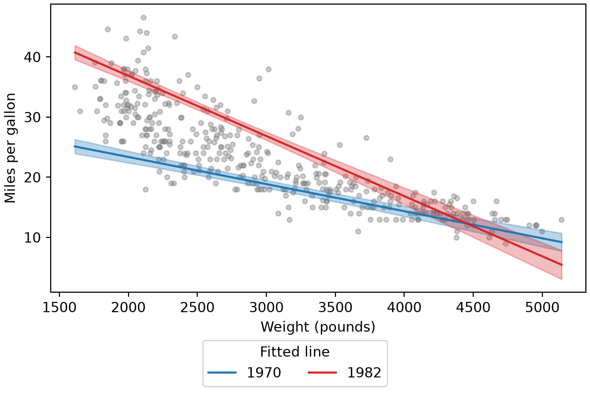
Figure 2: Fuel economy against weight for the Auto data, with the fitted lines of the interaction model for model years 1970 and 1982. Each shaded ribbon is the 95% confidence band for the mean fuel economy of cars of that model year.
Scatter plot of miles per gallon against weight for 392 cars, in grey. Two fitted lines slope down. The line for 1982 starts higher than the line for 1970 and falls more steeply, and the two lines cross near 4500 pounds. A shaded ribbon around each line shows its 95 percent confidence band, narrow in the middle of the weights and wider at the ends, and wide enough at the heavy end that the two ribbons overlap.
fit_weight_year <- lm(mpg ~ weight * year, data = auto)
parameters::parameters(fit_weight_year) |>
  parameters::print_md(digits = 4)
Parameter Coefficient SE 95% CI t(388) p
(Intercept) -110.4519 12.9470 (-135.9069, -84.9969) -8.5311 < .001
weight 0.0275 0.0044 (0.0189, 0.0362) 6.2415 < .001
year 2.0405 0.1718 (1.7027, 2.3783) 11.8756 < .001
weight × year -0.0005 5.9071e-05 (-0.0006, -0.0003) -7.7522 < .001
weight_slope <- function(model_year) {
  b <- coef(fit_weight_year)
  1000 * (b[["weight"]] + b[["weight:year"]] * model_year)
}
c(weight_slope(70), weight_slope(82))
[1]  -4.508741 -10.003929
# 95% confidence interval for the weight slope in a given model year:
# the slope is the linear combination a'b, with variance a' vcov a.
slope_ci <- function(model_year) {
  a <- 1000 * c(0, 1, 0, model_year)
  half <- qt(0.975, df.residual(fit_weight_year)) *
    sqrt(drop(t(a) %*% vcov(fit_weight_year) %*% a))
  sum(a * coef(fit_weight_year)) + c(-1, 1) * half
}
ci_interaction <- confint(fit_weight_year)["weight:year", ]
rbind(interaction = ci_interaction,
      slope_1970 = slope_ci(70), slope_1982 = slope_ci(82))
                    2.5 %        97.5 %
interaction -5.740726e-04 -0.0003417921
slope_1970  -5.175435e+00 -3.8420477515
slope_1982  -1.094509e+01 -9.0627664467
# The ratio of the two slopes is nonlinear in the coefficients, so bootstrap it:
# resample cars with replacement, refit, and recompute the ratio each time.
set.seed(571)
ratio_wy <- replicate(2000, {
  resampled <- auto[sample(nrow(auto), replace = TRUE), ]
  b <- coef(lm(mpg ~ weight * year, data = resampled))
  slope_82 <- b[["weight"]] + 82 * b[["weight:year"]]
  slope_70 <- b[["weight"]] + 70 * b[["weight:year"]]
  slope_82 / slope_70
})
ratio_ci_wy <- quantile(ratio_wy, c(0.025, 0.975))
ratio_ci_wy
    2.5%    97.5% 
1.814234 2.777316 
Show code
library(ggplot2)

weight_year_grid <- expand.grid(
  weight = seq(min(auto$weight), max(auto$weight), length.out = 100),
  year = c(70, 82)
)
# predict() returns the fit and the ends of its 95% confidence band.
band <- predict(fit_weight_year, weight_year_grid, interval = "confidence")
weight_year_grid <- cbind(weight_year_grid, band)
ggplot(auto, aes(weight, mpg)) +
  geom_point(colour = "grey50") +
  geom_ribbon(data = weight_year_grid,
              aes(y = NULL, ymin = lwr, ymax = upr, fill = factor(year + 1900)),
              alpha = 0.3) +
  geom_line(data = weight_year_grid,
            aes(y = fit, colour = factor(year + 1900)), linewidth = 1) +
  scale_colour_manual(values = c("steelblue", "firebrick")) +
  scale_fill_manual(values = c("steelblue", "firebrick")) +
  labs(x = "Weight (pounds)", y = "Miles per gallon",
       colour = "Fitted line", fill = "Fitted line")

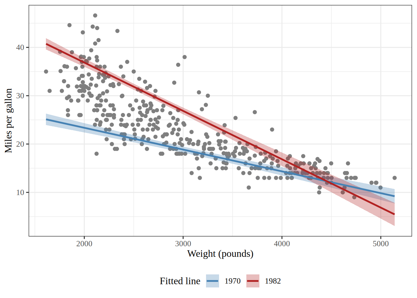
Scatter plot of miles per gallon against weight for 392 cars, drawn in R with ggplot2. Two fitted lines slope down. The line for 1982 starts higher than the line for 1970, falls more steeply, and crosses it near 4500 pounds. A shaded ribbon around each line shows its 95 percent confidence band, narrow in the middle of the weights and wider at the ends, and wide enough at the heavy end that the two ribbons overlap.

The interaction coefficient is \(\hcoef{3} = -4.6\times10^{-4}\), with a \(95\%\) confidence interval from \(-5.7\times10^{-4}\) to \(-3.4\times10^{-4}\). By Definition 1, the slope in weight is \(\hcoef{1} + \hcoef{3} \cdot \text{year}\). Per \(1000\) pounds, it is -4.5 miles per gallon for a \(1970\) car (interval -5.2 to -3.8) and -10.0 for a \(1982\) car (interval -10.9 to -9.1). The intervals for the coefficient and the slopes are model-based \(t\) intervals. In the fitted model, the estimated slope in weight for \(1982\) cars is about 2.2 times the estimated slope for \(1970\) cars (both slopes are negative), with a \(95\%\) bootstrap percentile interval for the ratio from 1.8 to 2.8. All of these intervals describe which cars were drawn, and assume the model’s form is right.

ExmExample 3 (The interaction term twists the fitted plane)

Example 3 (The interaction term twists the fitted plane) Fit mpg on weight and year twice: once without the interaction term, as an additive model, and once with it, as in Example 2.

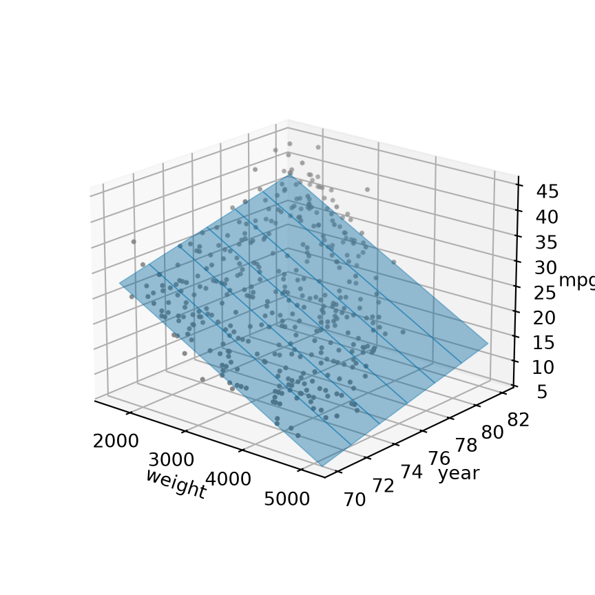
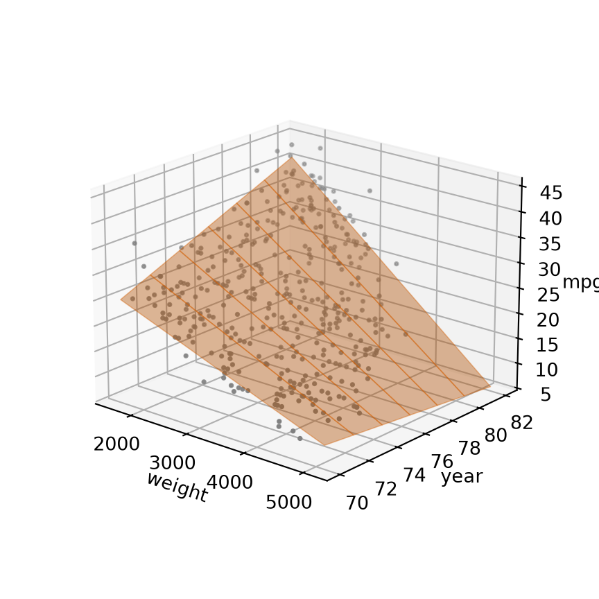
Figure 3 draws both fitted surfaces over the cars.

Figure 3: The fitted surfaces of two models for mpg over weight and year, with the cars as gray points.
Show code
# Both fitted surfaces on a grid of the two features.
wy_weight_range <- range(auto$weight)
wy_weights <- seq(wy_weight_range[[1]], wy_weight_range[[2]], length.out = 20)
wy_years <- 70:82
wy_grid <- tidyr::expand_grid(year = wy_years, weight = wy_weights)
wy_pred_additive <- predict(fit_wy_additive, newdata = wy_grid)
wy_pred_interaction <- predict(fit_weight_year, newdata = wy_grid)
# One row of heights for each year.
wy_nyears <- length(wy_years)
wy_z_additive <- matrix(wy_pred_additive, nrow = wy_nyears, byrow = TRUE)
wy_z_interaction <- matrix(wy_pred_interaction, nrow = wy_nyears, byrow = TRUE)
# One z range for both panels, holding the cars and both surfaces.
wy_zlim <- range(auto$mpg, wy_z_additive, wy_z_interaction)
wy_slice_rows <- seq(1, wy_nyears, by = 2)
wy_is_html <- knitr::is_html_output()

# Draws one fitted surface z (one row per year) over the cars, with its
# slices at every second model year: an interactive plotly widget in HTML,
# and the same picture from persp() in static formats.
# nolint start: function_location_linter. lds has no R/ directory.
wy_surface <- function(cars, z, fill, slice_colour, alt) {
  if (wy_is_html) {
    fills <- c(fill, fill)
    stops <- c(0, 1)
    scale <- list(stops, fills)
    slices <- list(
      show = TRUE, start = 70, end = 82, size = 2,
      color = slice_colour, width = 4
    )
    contours <- list(y = slices)
    marker <- list(size = 2, color = "grey")
    # A distant camera, aimed a little off centre, keeps every axis label
    # inside a half-width panel.
    eye <- list(x = 2.6, y = -2.6, z = 1.3)
    aim <- list(x = -0.15, y = -0.05, z = 0)
    camera <- list(eye = eye, center = aim)
    tick_font <- list(size = 9)
    title_font <- list(size = 11)
    weight_title <- list(text = "weight", font = title_font)
    year_title <- list(text = "year", font = title_font)
    mpg_title <- list(text = "mpg", font = title_font)
    xaxis <- list(title = weight_title, nticks = 4, tickfont = tick_font)
    yaxis <- list(title = year_title, nticks = 4, tickfont = tick_font)
    zaxis <- list(
      title = mpg_title, nticks = 4, tickfont = tick_font, range = wy_zlim
    )
    # The three axes have different units, so the box is a cube.
    scene <- list(
      xaxis = xaxis, yaxis = yaxis, zaxis = zaxis,
      camera = camera, aspectmode = "cube"
    )
    # Plotly's default margins would leave the half-width panel little room.
    no_margin <- list(l = 0, r = 0, t = 0, b = 0)
    widget <- plotly::plot_ly(height = 320) |>
      plotly::add_surface(
        x = wy_weights,
        y = wy_years,
        z = z,
        colorscale = scale,
        contours = contours,
        showscale = FALSE,
        opacity = 0.6
      ) |>
      plotly::add_trace(
        data = cars,
        type = "scatter3d",
        mode = "markers",
        x = ~weight,
        y = ~year,
        z = ~mpg,
        marker = marker
      ) |>
      plotly::layout(scene = scene, margin = no_margin, showlegend = FALSE)
    htmltools::div(role = "img", `aria-label` = alt, widget)
  } else {
    # persp() wants one row of heights for each weight.
    z_persp <- t(z)
    facet_fill <- adjustcolor(fill, 0.4)
    margins <- c(1, 1, 0, 1)
    flat <- list(mar = margins)
    withr::with_par(flat, {
      view <- persp(
        wy_weights, wy_years, z_persp,
        zlim = wy_zlim, theta = -35, phi = 25, expand = 0.8,
        col = facet_fill, border = NA, ticktype = "detailed", nticks = 4,
        xlab = "weight", ylab = "year", zlab = "mpg",
        cex.axis = 0.7, cex.lab = 0.8
      )
      for (k in wy_slice_rows) {
        year_k <- wy_years[[k]]
        slice <- trans3d(wy_weights, year_k, z_persp[, k], view)
        lines(slice, col = slice_colour, lwd = 1.5)
      }
      car_points <- trans3d(cars$weight, cars$year, cars$mpg, view)
      points(car_points, pch = 16, cex = 0.3, col = "grey40")
    })
  }
}
# nolint end

wy_surface(auto, wy_z_additive, "#0072B2", "#003F63", wy_alt_additive)
Show code
beta_wy_additive, Phi_wy_additive = fit([weight, year])
grid_weight, grid_year = np.meshgrid(
    np.linspace(weight.min(), weight.max(), 20),
    np.arange(70, 83),
)
surface_additive = (
    beta_wy_additive[0]
    + beta_wy_additive[1] * grid_weight
    + beta_wy_additive[2] * grid_year
)
surface_interaction = (
    beta_weight_year[0]
    + beta_weight_year[1] * grid_weight
    + beta_weight_year[2] * grid_year
    + beta_weight_year[3] * grid_weight * grid_year
)
# One z range for both panels, holding the cars and both surfaces.
z_min = min(y.min(), surface_additive.min(), surface_interaction.min())
z_max = max(y.max(), surface_additive.max(), surface_interaction.max())

def plot_wy_surface(surface, colour):
    """Draw one fitted surface over weight and year, with its slices and the cars."""
    fig = plt.figure(figsize=(4.5, 4.5), layout="constrained")
    ax = fig.add_subplot(projection="3d")
    # Edges every two model years draw the slices at fixed values of year.
    ax.plot_surface(grid_weight, grid_year, surface, color=colour, alpha=0.4,
                    edgecolor=colour, linewidth=0.6, rstride=2, cstride=19);
    ax.scatter(weight, year, y, color="grey", s=3);
    ax.set_xlabel("weight");
    ax.set_ylabel("year");
    ax.set_zlabel("mpg");
    ax.set_zlim(z_min, z_max);
    ax.set_xticks([2000, 3000, 4000, 5000]);
    ax.view_init(elev=20, azim=-50);
    ax.set_box_aspect(None, zoom=0.8);
    plt.show()

plot_wy_surface(surface_additive, "#0072B2")
(a) Without the interaction term: the surface is a plane, and its slices at every second value of year are parallel.

3D plot of miles per gallon against weight and model year for the Auto cars, drawn as grey points, with the additive model's fitted surface: a flat plane whose slices at every second model year are parallel lines.


Show code
wy_surface(auto, wy_z_interaction, "#D55E00", "#8A3C00", wy_alt_interaction)
Show code
plot_wy_surface(surface_interaction, "#D55E00")
(b) With the interaction term: the surface twists, and its slices at every second value of year fan out.

3D plot of miles per gallon against weight and model year for the Auto cars, drawn as grey points, with the interaction model's fitted surface: a twisted surface whose slices at every second model year fan out, falling more steeply with weight for later model years.

In the additive model (Figure 3 (a)), the slope in weight is -6.6 miles per gallon per \(1000\) pounds in every model year. So the slices of the surface at fixed values of year are parallel lines, and the surface is a plane. With the interaction term (Figure 3 (b)), the slope in weight is \(\hcoef{1} + \hcoef{3} \cdot \text{year}\), which goes from -4.5 per \(1000\) pounds in \(1970\) to -10.0 in \(1982\). The slices at different years have different slopes, so the surface twists and is no longer a plane.

DefDefinition 2 (Hierarchy principle (hierarchical principle))

Definition 2 (Hierarchy principle (hierarchical principle)) The hierarchy principle (also called the hierarchical principle) says that a model with an interaction \(x_1 x_2\) should also include the main effects \(x_1\) and \(x_2\) [1, Sec. 3.3.2].

ExmExample 4 (Weight and year in the Auto data)

Example 4 (Weight and year in the Auto data) The model of mpg with the interaction weight \(\times\) year and the main effects weight and year follows the principle. The model of mpg with weight \(\times\) year and weight but without year does not. It forces the effect of model year on mpg to be zero for a car that weighs nothing, which no car does.

PrpProposition 1 (A model with its main effects is unchanged by shifting a feature)

Proposition 1 (A model with its main effects is unchanged by shifting a feature) Call a function a model function if it has the form \(b_0 + b_1 x_1 + b_2 x_2 + b_3 x_1 x_2\), for some coefficients \(b_0, b_1, b_2, b_3\). Shifting \(x_1\) by a constant \(c\), to \(x_1' = x_1 + c\), turns every model function into a model function of \(x_1'\) and \(x_2\).

Proof. For a shift of \(x_1\), substitute \(x_1 = x_1' - c\).

\[ b_0 + b_1 (x_1' - c) + b_2 x_2 + b_3 (x_1' - c) x_2 = (b_0 - c b_1) + b_1 x_1' + (b_2 - c b_3) x_2 + b_3 x_1' x_2, \]

which has the form of a model function in \(x_1'\) and \(x_2\). The same substitution, with the roles of \(x_1\) and \(x_2\) exchanged, shows the same for a shift of \(x_2\).

ExmExample 5 (Centering weight in the Auto data)

Example 5 (Centering weight in the Auto data) Take the model of mpg with weight \(\times\) year and both main effects. Subtract a constant \(c\) from weight, as when centering weight at a typical value. By Proposition 1, the model is still a model function of the shifted weight and year. The fitted model does not change, because adding \(c\) back to weight undoes the shift, so the model functions before and after the shift are the same. Only the coefficients change, and the coefficient of year becomes the effect of model year on mpg for a car with weight \(= c\).

PrpProposition 2 (Shifting a feature can create a dropped main effect)

Proposition 2 (Shifting a feature can create a dropped main effect) Let a function without the main effect of \(x_1\) have the form \(b_0 + b_2 x_2 + b_3 x_1 x_2\), with \(b_3 \neq 0\). Shifting \(x_2\) by a constant \(c \neq 0\), to \(x_2' = x_2 + c\), gives a function with a nonzero main effect of \(x_1\).

Proof. Substitute \(x_2 = x_2' - c\).

\[ b_0 + b_2 (x_2' - c) + b_3 x_1 (x_2' - c) = (b_0 - c b_2) + b_2 x_2' + b_3 x_1 x_2' - c b_3 x_1. \]

Here \(- c b_3 x_1\) is a main effect of \(x_1\), with the coefficient \(- c b_3\), which is nonzero because \(b_3 \neq 0\) and \(c \neq 0\). So the shifted function is not of the form without the main effect of \(x_1\).

ExmExample 6 (Shifting weight without the main effect of year)

Example 6 (Shifting weight without the main effect of year) Take the model of mpg with weight and weight \(\times\) year, but without year. Add a constant \(c \neq 0\) to weight. By Proposition 2, the shifted model has a main effect of year, with the coefficient \(- c\) times that of weight \(\times\) year. So the model that followed the hierarchy principle before the shift no longer does.

3 Inference for the coefficients

This section follows [1, Sec. 3.1.2], and takes the matrix form of the results from the rme notes on linear models.

3.1 How precise is a coefficient?

ExrExercise 2 (How much would the slope change with new data?)

Exercise 2 (How much would the slope change with new data?) The one-feature fit has a slope of -0.158 miles per gallon per horsepower to \(392\) cars. Suppose we measured \(392\) different cars of the same kinds and fitted the same model. Would we get the same slope?

Solution 2. No. Each response is \(y_i = \dprod{\phi(\vx_i)}{\vcoef} + \err_i\), and the noise terms \(\err_i\) differ from one sample to the next. The estimate \(\hvcoef = (\stprod{\design})^{-1} \tp{\design} \vy\) is a function of \(\vy\), so it is a random variable too.

ExrExercise 3 (How much would the slope change with new data? (part 2))

Exercise 3 (How much would the slope change with new data? (part 2)) Use the setup of Exercise 2.

What would describe how much the slope changes from one sample of cars to another?

Solution 3. The standard deviation of \(\hcoef{1}\) over repeated samples describes how much the slope changes. A small standard deviation shows that one sample pins the slope down well.

3.2 The covariance of the least squares estimate

ExrExercise 4 (The mean and covariance of the least squares estimate)

Exercise 4 (The mean and covariance of the least squares estimate) Suppose \(\vy = \design \vcoef + \veps\), where \(\design\) is a fixed \(n \times p^*\) design matrix with full column rank, \(\E{\veps} = \mathbf{0}_{n \times 1}\) and \(\Cov{\veps} = \sigma^2 \mathbf{I}_n\). Find the mean \(\E{\hvcoef}\) and the covariance matrix \(\Cov{\hvcoef}\) of the least squares estimate \(\hvcoef = (\stprod{\design})^{-1} \tp{\design} \vy\).

TipHint

First write \(\hvcoef - \vcoef\) as a matrix times \(\veps\).

Solution 4. Let \(\mathbf{A} = (\stprod{\design})^{-1} \tp{\design}\), a fixed \(p^* \times n\) matrix. Substitute the model for \(\vy\):

\[ \begin{aligned} \hvcoef &= \mathbf{A} (\design \vcoef + \veps) && \text{(substitute } \vy = \design\vcoef + \veps \text{)} \\ &= (\stprod{\design})^{-1} \stprod{\design} \vcoef + \mathbf{A} \veps && \text{(distribute)} \\ &= \vcoef + \mathbf{A} \veps && \text{(} (\stprod{\design})^{-1} \stprod{\design} = \mathbf{I}_{p^*} \text{)} \end{aligned} \]

The mean follows from linearity of expectation:

\[ \begin{aligned} \E{\hvcoef} &= \vcoef + \mathbf{A} \, \E{\veps} && \text{(linearity; } \mathbf{A} \text{ is fixed)} \\ &= \vcoef && \text{(} \E{\veps} = \mathbf{0} \text{)} \end{aligned} \]

So \(\hvcoef\) is unbiased. For the covariance, \(\hvcoef - \E{\hvcoef} = \mathbf{A}\veps\):

\[ \begin{aligned} \Cov{\hvcoef} &= \E{(\mathbf{A}\veps)\pt{\mathbf{A}\veps}} && \text{(definition of covariance)} \\ &= \E{\mathbf{A} \veps \tp{\veps} \mathbf{A}^\top} && \text{(} \pt{\mathbf{A}\veps} = \tp{\veps} \mathbf{A}^\top \text{)} \\ &= \mathbf{A} \, \E{\veps \tp{\veps}} \mathbf{A}^\top && \text{(linearity; } \mathbf{A} \text{ is fixed)} \\ &= \mathbf{A} \, (\sigma^2 \mathbf{I}_n) \, \mathbf{A}^\top && \text{(} \E{\veps \tp{\veps}} = \Cov{\veps} \text{, since } \E{\veps} = \mathbf{0} \text{)} \\ &= \sigma^2 (\stprod{\design})^{-1} \stprod{\design} (\stprod{\design})^{-1} && \text{(} \mathbf{A}^\top = \design (\stprod{\design})^{-1} \text{, as } \stprod{\design} \text{ is symmetric)} \\ &= \sigma^2 (\stprod{\design})^{-1} && \text{(} \stprod{\design} (\stprod{\design})^{-1} = \mathbf{I}_{p^*} \text{)} \end{aligned} \]

LemTheorem 1 (Mean and covariance of the least squares estimate)

Theorem 1 (Mean and covariance of the least squares estimate) If \(\vy = \design \vcoef + \veps\) with \(\design\) fixed and of full column rank, \(\E{\veps} = \mathbf{0}_{n \times 1}\) and \(\Cov{\veps} = \sigma^2 \mathbf{I}_n\), then

\[ \E{\hvcoef} = \vcoef, \qquad \Cov{\hvcoef} = \sigma^2 \underbrace{(\stprod{\design})^{-1}}_{p^* \times p^*}. \]

In particular, \(\Var{\hcoef{j}} = \sigma^2 \sb{(\stprod{\design})^{-1}}_{jj}\).

Proof. By Solution 4.

ExmExample 7 (Checking the slope’s variance by simulation)

Example 7 (Checking the slope’s variance by simulation) Take the design matrix of the one-feature fit (an intercept and horsepower for the \(392\) Auto cars), treat its fitted coefficients as the true \(\vcoef\), and take \(\sigma\) to be its residual standard error. Simulate \(2000\) new response vectors \(\vy = \design\vcoef + \veps\) with \(\veps \sim \Normal(\mathbf{0}, \sigma^2 \mathbf{I}_n)\), refit each one, and compare the standard deviation of the \(2000\) slopes with \(\sqrt{\sigma^2 [(\stprod{\design})^{-1}]_{11}}\) from Theorem 1:

residuals_simple = y - Phi_simple @ beta_simple
sigma_simple = np.sqrt(np.sum(residuals_simple ** 2) / (n - 2))
PtP_inv = np.linalg.inv(Phi_simple.T @ Phi_simple)
sd_theory = sigma_simple * np.sqrt(PtP_inv[1, 1])

rng = np.random.default_rng(571)
n_sims = 2000
sim_slopes = np.empty(n_sims)
sim_ses = np.empty(n_sims)
for sim in range(n_sims):
    y_sim = Phi_simple @ beta_simple + rng.normal(0, sigma_simple, n)
    b_sim = PtP_inv @ Phi_simple.T @ y_sim
    rse_sim = np.sqrt(np.sum((y_sim - Phi_simple @ b_sim) ** 2) / (n - 2))
    sim_slopes[sim] = b_sim[1]
    sim_ses[sim] = rse_sim * np.sqrt(PtP_inv[1, 1])

from scipy import stats

# The simulated slopes are exactly Gaussian, so (N - 1) s^2 / sd^2 follows
# a chi-squared distribution with N - 1 degrees of freedom;
# inverting that statement gives a 95% interval for the true standard deviation.
sd_sim = np.std(sim_slopes, ddof=1)
sd_sim_ci = sd_sim * np.sqrt((n_sims - 1) / stats.chi2.ppf([0.975, 0.025], df=n_sims - 1))
print(sd_theory, sd_sim, sd_sim_ci)
0.006445500517685036 0.006482351093736395 [0.00628751 0.00668974]
design <- model.matrix(fit_simple)
sigma_simple <- summary(fit_simple)$sigma
xtx_inv <- solve(crossprod(design))
sd_theory <- sigma_simple * sqrt(xtx_inv[2, 2])

set.seed(571)
sim_fits <- replicate(2000, {
  y_sim <- fitted(fit_simple) + rnorm(nrow(design), 0, sigma_simple)
  coef(summary(lm(y_sim ~ design - 1)))[2, c("Estimate", "Std. Error")]
})
sd_sim <- sd(sim_fits["Estimate", ])
n_sims <- ncol(sim_fits)
# The simulated slopes are exactly Gaussian, so (N - 1) s^2 / sd^2 follows
# a chi-squared distribution with N - 1 degrees of freedom;
# inverting that statement gives a 95% interval for the true standard deviation.
chi_sq <- qchisq(c(0.975, 0.025), df = n_sims - 1)
sd_sim_ci <- sd_sim * sqrt((n_sims - 1) / chi_sq)
c(theory = sd_theory, simulated = sd_sim,
  lower = sd_sim_ci[1], upper = sd_sim_ci[2])
     theory   simulated       lower       upper 
0.006445501 0.006367362 0.006175978 0.006571075 

The formula gives 0.00645, and the \(2000\) simulated slopes have standard deviation 0.00648, with a \(95\%\) confidence interval from 0.00629 to 0.00669. The interval measures only the simulation error of using \(2000\) draws, and it uses the exact chi-squared distribution of a Gaussian sample’s variance. The formula’s value lies inside it, so the two agree to within simulation error.

3.3 Standard errors

DefDefinition 3 (Standard error of a coefficient)

Definition 3 (Standard error of a coefficient) The standard error of \(\hcoef{j}\) is its standard deviation over repeated samples,

\[ \SE{\hcoef{j}} = \sigma \sqrt{\sb{(\stprod{\design})^{-1}}_{jj}}, \]

by Theorem 1.

ExmExample 8 (Standard errors when \(\sigma\) is known)

Example 8 (Standard errors when \(\sigma\) is known) In the simulation of Example 7, the noise level \(\sigma\) is known, so we can compute the standard errors of Definition 3 exactly:

se_known_sigma = sigma_simple * np.sqrt(np.diag(PtP_inv))
print(se_known_sigma)
[0.71749866 0.0064455 ]
se_known_sigma <- sigma_simple * sqrt(diag(xtx_inv))
se_known_sigma
(Intercept)  horsepower 
0.717498656 0.006445501 

The slope’s standard error is 0.00645. It is one fixed number for the whole simulation, and it matches the spread of the \(2000\) simulated slopes, whose standard deviation is 0.00648.

DefDefinition 4 (Estimated standard error)

Definition 4 (Estimated standard error) In practice the noise level \(\sigma\) in Definition 3 is unknown. Replacing it by the residual standard error, \(\hat\sigma = \text{RSE}\), gives the estimated standard error

\[ \hse{\hcoef{j}} = \hat\sigma \sqrt{\sb{(\stprod{\design})^{-1}}_{jj}}. \]

Software output, and most books, call \(\hse{\hcoef{j}}\) “the standard error” too [1, Sec. 3.1.2], p. 75.

ExmExample 9 (The slope’s estimated standard error for the Auto data)

Example 9 (The slope’s estimated standard error for the Auto data) For the one-feature fit, compute \(\hse{\hcoef{1}}\) from Definition 4, and compare it with the standard error in the table from R’s parameters package:

se_simple = sigma_simple * np.sqrt(np.diag(PtP_inv))
print(se_simple)
[0.71749866 0.0064455 ]
se_by_hand <- sigma_simple * sqrt(diag(xtx_inv))
se_by_hand
(Intercept)  horsepower 
0.717498656 0.006445501 
parameters::parameters(fit_simple) |>
  parameters::print_md(digits = 4)
Parameter Coefficient SE 95% CI t(390) p
(Intercept) 39.9359 0.7175 (38.5252, 41.3465) 55.6598 < .001
horsepower -0.1578 0.0064 (-0.1705, -0.1452) -24.4891 < .001

The residual standard error is \(\hat\sigma =\) 4.91, and \(\hse{\hcoef{1}} =\) 0.00645, the same value as the standard error column of the parameters table. It also equals the standard error of Example 8, because that simulation set \(\sigma\) to this same \(\hat\sigma\). The slope \(\hcoef{1} =\) -0.158 is about 24 standard errors away from \(0\).

Unlike the standard error, the estimate changes from one data set to the next. Across the \(2000\) simulated data sets of Example 7, \(\hse{\hcoef{1}}\) ranges from 0.0057 to 0.00727, around the standard error 0.00645 of Example 8.

3.4 The \(t\) distribution of a coefficient

LemTheorem 2 (The standardized coefficient has a \(t\) distribution)

Theorem 2 (The standardized coefficient has a \(t\) distribution) Under the assumptions of Theorem 1, suppose also that the noise is Gaussian, \(\veps \sim \Normal(\mathbf{0}, \sigma^2 \mathbf{I}_n)\). Then for each coefficient,

\[ T_j = \frac{\hcoef{j} - \coef{j}}{\hse{\hcoef{j}}} \sim t_{n - p^*}, \]

the \(t\) distribution with \(n - p^*\) degrees of freedom [1, Sec. 3.1.2], p. 77.

The proof needs the distribution of \(\hat\sigma^2\) and its independence from \(\hvcoef\), which these notes do not cover. James et al. [1, Sec. 3.1.2] states the result for simple linear regression, and the rme notes state it for multiple regression.

ExmExample 10 (Checking the \(t\) distribution by simulation)

Example 10 (Checking the \(t\) distribution by simulation) For each of the \(2000\) simulated samples of Example 7, compute \(T_1 = (\hcoef{1} - \coef{1}) / \hse{\hcoef{1}}\). By Theorem 2, about \(5\%\) of them should land outside \(\pm t_{n-2}(0.975)\), the \(97.5\)th percentile of \(t_{n-2}\):

from scipy import stats

t_sim = (sim_slopes - beta_simple[1]) / sim_ses
t_crit = stats.t.ppf(0.975, df=n - 2)
n_outside = int(np.sum(np.abs(t_sim) > t_crit))
# An exact (Clopper-Pearson) 95% interval for the proportion outside.
outside_ci = stats.binomtest(n_outside, len(t_sim)).proportion_ci(
    confidence_level=0.95, method="exact")
outside_lo, outside_hi = outside_ci.low, outside_ci.high
print(t_crit, n_outside / len(t_sim), outside_lo, outside_hi)
1.9660653313011052 0.0495 0.04041037792654773 0.05993731615842642
t_sim <- (sim_fits["Estimate", ] - coef(fit_simple)[["horsepower"]]) /
  sim_fits["Std. Error", ]
t_crit <- qt(0.975, df = fit_simple$df.residual)
n_outside <- sum(abs(t_sim) > t_crit)
# binom.test gives an exact (Clopper-Pearson) 95% interval
# for the proportion outside.
outside_ci <- binom.test(n_outside, length(t_sim))$conf.int
c(t_crit = t_crit, outside = n_outside / length(t_sim),
  lower = outside_ci[1], upper = outside_ci[2])
    t_crit    outside      lower      upper 
1.96606533 0.04400000 0.03543624 0.05393046 

With \(n - 2 =\) 390 degrees of freedom, \(t_{n-2}(0.975) =\) 1.966, and 5.0% of the simulated \(T_1\) values land outside \(\pm\) 1.966, with an exact \(95\%\) confidence interval for that proportion from 4.0% to 6.0%. The interval covers the nominal \(5\%\), and it measures only the simulation error of \(2000\) draws.

3.5 Confidence intervals

ExrExercise 5 (An interval that catches the true coefficient)

Exercise 5 (An interval that catches the true coefficient) Use Theorem 2 to find an interval, computed from the data, that contains the true \(\coef{j}\) with probability \(0.95\).

Solution 5. Write \(c = t_{n-p^*}(0.975)\) for the \(97.5\)th percentile of \(t_{n-p^*}\). By Theorem 2, \(T_j \sim t_{n-p^*}\), and the \(t\) distribution is symmetric about \(0\), so

\[ \begin{aligned} 0.95 &= \Pf{-c \le T_j \le c} && \text{(definition of } c \text{; symmetry)} \\ &= \Pf{-c \le \frac{\hcoef{j} - \coef{j}}{\hse{\hcoef{j}}} \le c} && \text{(definition of } T_j \text{)} \\ &= \Pf{-c \, \hse{\hcoef{j}} \le \hcoef{j} - \coef{j} \le c \, \hse{\hcoef{j}}} && \text{(multiply by } \hse{\hcoef{j}} > 0 \text{)} \\ &= \Pf{\hcoef{j} - c \, \hse{\hcoef{j}} \le \coef{j} \le \hcoef{j} + c \, \hse{\hcoef{j}}} && \text{(rearrange for } \coef{j} \text{)} \end{aligned} \]

So the interval \(\hcoef{j} \pm c \, \hse{\hcoef{j}}\) contains \(\coef{j}\) with probability \(0.95\). The interval is random, and \(\coef{j}\) is fixed.

LemTheorem 3 (The coefficient interval has probability \(0.95\) of containing the coefficient)

Theorem 3 (The coefficient interval has probability \(0.95\) of containing the coefficient) Let \(c = t_{n-p^*}(0.975)\). Under the assumptions of Theorem 2,

\[ \Pf{\hcoef{j} - c \, \hse{\hcoef{j}} \le \coef{j} \le \hcoef{j} + c \, \hse{\hcoef{j}}} = 0.95. \]

The interval is random, and \(\coef{j}\) is fixed.

Proof. This is the solution to Exercise 5: see Solution 5.

ExmExample 11 (Coverage of the coefficient interval in simulation)

Example 11 (Coverage of the coefficient interval in simulation) Simulate \(5000\) data sets of \(n = 30\) points from \(y = 1 + 2x + \err\) with \(\err \sim \ndist{0, 1}\). For each, build the \(95\%\) interval for the slope of Definition 5 and check whether it contains the true slope \(2\).

Show code
# Save and restore the random seed, so this example does not change later random output.
ci_old_seed <- if (exists(".Random.seed", globalenv())) get(".Random.seed", globalenv())
set.seed(571)
ci_covered <- replicate(5000, {
  x <- runif(30)
  y <- 1 + 2 * x + rnorm(30)
  ci <- confint(lm(y ~ x))["x", ]
  ci[1] <= 2 && 2 <= ci[2]
})
if (!is.null(ci_old_seed)) assign(".Random.seed", ci_old_seed, globalenv())
mean(ci_covered)
[1] 0.9532

The intervals contain the true slope in 95.3% of the data sets, close to the stated \(95\%\).

DefDefinition 5 (Confidence interval for a coefficient)

Definition 5 (Confidence interval for a coefficient) The \(95\%\) confidence interval for \(\coef{j}\) is

\[ \hcoef{j} \pm t_{n - p^*}(0.975) \, \hse{\hcoef{j}}. \]

Over repeated samples, \(95\%\) of the intervals built this way contain the true \(\coef{j}\), by Theorem 3. For large \(n\), \(t_{n - p^*}(0.975)\) is close to \(2\), and James et al. [1, Sec. 3.1.2], p. 75 writes the interval as \(\hcoef{j} \pm 2 \, \hse{\hcoef{j}}\).

ExmExample 12 (A confidence interval for the horsepower slope)

Example 12 (A confidence interval for the horsepower slope) Compute the \(95\%\) confidence interval for the slope of the one-feature fit from Definition 5, and compare it with the 95% confidence interval columns of the table from R’s parameters package:

ci_slope = beta_simple[1] + np.array([-1, 1]) * t_crit * se_simple[1]
print(ci_slope)
[-0.17051701 -0.14517246]
coef(fit_simple)[["horsepower"]] + c(-1, 1) * t_crit * se_by_hand[[2]]
[1] -0.1705170 -0.1451725
parameters::parameters(fit_simple) |>
  parameters::print_md(digits = 4, ci_digits = 4)
Parameter Coefficient SE 95% CI t(390) p
(Intercept) 39.9359 0.7175 (38.5252, 41.3465) 55.6598 < .001
horsepower -0.1578 0.0064 (-0.1705, -0.1452) -24.4891 < .001

The interval runs from -0.171 to -0.145 miles per gallon per horsepower. Every value in the interval is negative, so the interval excludes a slope of zero.

3.6 Testing whether a coefficient is zero

DefDefinition 6 (The \(t\)-test for a coefficient)

Definition 6 (The \(t\)-test for a coefficient) To test the null hypothesis \(H_0: \coef{j} = 0\) (feature \(j\) adds nothing to the model that already contains the other features) against \(H_A: \coef{j} \neq 0\), compute the \(t\)-statistic

\[ t_j = \frac{\hcoef{j}}{\hse{\hcoef{j}}}. \]

Under \(H_0\), \(t_j\) has the \(t_{n-p^*}\) distribution, by Theorem 2. The \(p\)-value is the probability, under \(H_0\), of a statistic at least as far from \(0\):

\[ \begin{aligned} p &= \Pf{\abs{T_{n-p^*}} \ge |t_j|} \\ &= 2 \, \Pf{T_{n-p^*} \ge |t_j|}. \end{aligned} \]

A small \(p\)-value is evidence against \(H_0\) [1, Sec. 3.1.2], p. 77.

ExmExample 13 (Does horsepower matter once weight is in the model?)

Example 13 (Does horsepower matter once weight is in the model?) For the two-feature fit, compute the \(t\)-statistic and \(p\)-value for horsepower from Definition 6, and compare them with the table from R’s parameters package:

p_star = Phi_multiple.shape[1]
rse_multiple = np.sqrt(
    np.sum((y - Phi_multiple @ beta_multiple) ** 2) / (n - p_star)
)
se_multiple = rse_multiple * np.sqrt(
    np.diag(np.linalg.inv(Phi_multiple.T @ Phi_multiple))
)
t_multiple = beta_multiple / se_multiple
p_multiple = 2 * stats.t.sf(np.abs(t_multiple), df=n - p_star)
print(t_multiple)
[ 57.5396503   -4.26725251 -11.53463263]
print(p_multiple)
[2.31711323e-192 2.48848204e-005 1.12436236e-026]
parameters::parameters(fit_multiple) |>
  parameters::print_md(digits = 4)
Parameter Coefficient SE 95% CI t(389) p
(Intercept) 45.6402 0.7932 (44.0807, 47.1997) 57.5397 < .001
horsepower -0.0473 0.0111 (-0.0691, -0.0255) -4.2673 < .001
weight -0.0058 0.0005 (-0.0068, -0.0048) -11.5346 < .001

For horsepower, \(t =\) -4.27 with \(n - p^* =\) 389 degrees of freedom, so \(p = 2.5\times10^{-5}\). Even with weight held fixed, the data are unlikely under \(H_0: \coef{\text{hp}} = 0\). The \(t\)-statistic for horsepower is much smaller in size than in the one-feature fit, where it was -24.5, because horsepower and weight carry much of the same information.

3.7 Is any feature useful?

ExrExercise 6 (Why not just check each \(t\)-test?)

Exercise 6 (Why not just check each \(t\)-test?) Suppose a model has \(p = 100\) features, and none of them is related to the response:

\[ \begin{aligned} \coef{1} &= \coef{2} \\ &= \cdots \\ &= \coef{100} \\ &= 0. \end{aligned} \]

We run the \(t\)-test of Definition 6 on each coefficient at level \(0.05\). About how many of the \(100\) \(p\)-values will fall below \(0.05\)?

Solution 6. Under \(H_0: \coef{j} = 0\), each \(p\)-value falls below \(0.05\) with probability \(0.05\). So we expect about \(100 \times 0.05 = 5\) of them to fall below \(0.05\) by chance, even though no feature is related to the response.

ExrExercise 7 (Why not just check each \(t\)-test? (part 2))

Exercise 7 (Why not just check each \(t\)-test? (part 2)) Use the setup of Exercise 6.

What does that say about using the separate \(t\)-tests to decide whether any feature is related to the response?

Solution 7. If we declared a relationship whenever any one \(p\)-value was small, we would almost always find one. We need a single test of all the coefficients together, whose chance of a false alarm is \(0.05\) no matter how many features there are [1, Sec. 3.2.2], p. 86.

DefDefinition 7 (The \(F\)-test that any feature is useful)

Definition 7 (The \(F\)-test that any feature is useful) To test

\[ H_0: \coef{j} = 0 \text{ for every } j \in \{1, \ldots, p\} \quad \text{against} \quad H_A: \text{at least one } \coef{j} \neq 0, \]

compute the \(F\)-statistic

\[ F = \frac{(\text{TSS} - \text{RSS}) / p}{\text{RSS} / (n - p - 1)}, \]

where \(\text{TSS} = \sum_i (y_i - \bar{y})^2\) is the total sum of squares and \(\text{RSS} = \sum_i (y_i - \hat{y}_i)^2\) is the residual sum of squares [1, Sec. 3.2.2], p. 84. If \(H_0\) holds and the noise is Gaussian, \(F\) has the \(F\) distribution with \(p\) and \(n - p - 1\) degrees of freedom [1, Sec. 3.2.2], p. 85. The \(p\)-value is \(\Pf{F_{p, n-p-1} \ge F}\).

The numerator is the drop in squared error per feature, and the denominator is \(\hat\sigma^2\), the squared residual standard error. Under \(H_0\), both estimate \(\sigma^2\), so \(F\) is near \(1\); when some feature is useful, the numerator is larger, and so is \(F\).

ExmExample 14 (The \(F\)-test for horsepower and weight)

Example 14 (The \(F\)-test for horsepower and weight) For the two-feature fit, compute \(F\) and its \(p\)-value from Definition 7, and compare them with the \(F\)-statistic that broom::glance() reports in R:

tss = np.sum((y - y.mean()) ** 2)
rss_multiple = np.sum((y - Phi_multiple @ beta_multiple) ** 2)
p_features = 2
f_multiple = ((tss - rss_multiple) / p_features) / (
    rss_multiple / (n - p_features - 1)
)
print(f_multiple, stats.f.sf(f_multiple, p_features, n - p_features - 1))
467.91015349994683 3.059606299669705e-104
broom::glance(fit_multiple) |>
  dplyr::select(statistic, p.value, df, df.residual)

\(F =\) 467.9 on \(2\) and 389 degrees of freedom, far above \(1\). Its \(p\)-value is below \(10^{-100}\), so at least one of horsepower and weight is related to mpg.

3.8 Testing a group of features

DefDefinition 8 (The partial \(F\)-test for a group of features)

Definition 8 (The partial \(F\)-test for a group of features) To test whether a group of \(q\) features adds anything to a model that already contains the other \(p - q\), fit the model twice: once with all \(p\) features, with residual sum of squares \(\text{RSS}\), and once without the \(q\) features, with residual sum of squares \(\text{RSS}_0\). The partial \(F\)-statistic is

\[ F = \frac{(\text{RSS}_0 - \text{RSS}) / q}{\text{RSS} / (n - p - 1)} \]

[1, Sec. 3.2.2], p. 85. If the \(q\) coefficients are all \(0\) and the noise is Gaussian, \(F\) has the \(F_{q, n-p-1}\) distribution. Definition 7 is the case \(q = p\), where the smaller model has only an intercept and \(\text{RSS}_0 = \text{TSS}\). With \(q = 1\), the partial \(F\)-statistic is the square of that feature’s \(t\)-statistic.

The rme notes derive this test and connect it to the likelihood ratio test; see the partial \(F\)-test.

ExmExample 15 (Does origin matter once weight is known?)

Example 15 (Does origin matter once weight is known?) The origin fit fits mpg on weight and the two origin indicators. Test whether the two indicators together add anything to weight alone, so \(q = 2\) and \(p = 3\):

beta_weight, Phi_weight = fit([weight])
rss_0 = np.sum((y - Phi_weight @ beta_weight) ** 2)
rss_1 = np.sum((y - Phi_origin_weight @ beta_origin_weight) ** 2)
f_origin = ((rss_0 - rss_1) / 2) / (rss_1 / (n - 3 - 1))
print(f_origin, stats.f.sf(f_origin, 2, n - 3 - 1))
6.126802214577667 0.002400578748351605
fit_weight <- lm(mpg ~ weight, data = auto)
anova(fit_weight, fit_origin_weight) |>
  parameters::parameters() |>
  parameters::print_md(footer = "")
Parameter RSS Sum_Squares df df (error) Mean_Square F p
Model 1: mpg ~ weight 7321.23 390
Model 2: mpg ~ weight + factor(origin) 7097.10 224.14 2 388 112.07 6.13 0.002

\(F =\) 6.13 on \(2\) and 388 degrees of freedom, with \(p =\) 0.0024. The data are unlikely if origin adds nothing once weight is known, even though the Auto lab found that weight explains much of the raw gap between origins.

3.9 Confidence and prediction intervals

ExrExercise 8 (Two questions about a \(98\)-horsepower car)

Exercise 8 (Two questions about a \(98\)-horsepower car) The one-feature fit predicts 24.5 miles per gallon for a car with \(98\) horsepower. Which sources of error make that number uncertain as an estimate of the average mpg of all \(98\)-horsepower cars?

Solution 8. In Exercise 8, the average mpg at \(98\) horsepower is \(\dprod{\phi(\vx_0)}{\vcoef}\), with \(\phi(\vx_0) = \tp{[1, 98]}\). Its estimate \(\dprod{\phi(\vx_0)}{\hvcoef}\) is off only because \(\hvcoef\) differs from \(\vcoef\): the reducible error of the error decomposition.

ExrExercise 9 (Two questions about a \(98\)-horsepower car (part 2))

Exercise 9 (Two questions about a \(98\)-horsepower car (part 2)) Use the setup of Exercise 8. Which sources of error make that number uncertain as a guess at the mpg of one particular \(98\)-horsepower car?

Solution 9. One car’s mpg is \(\outvar_0 = \dprod{\phi(\vx_0)}{\vcoef} + \err_0\). The guess has the same error from \(\hvcoef\), plus the car’s own noise \(\err_0\), whose variance is the residual variance.

ExrExercise 10 (Two questions about a \(98\)-horsepower car (part 3))

Exercise 10 (Two questions about a \(98\)-horsepower car (part 3)) Use the setup of Exercise 8. Which of the two should we be less sure about?

Solution 10. We should be less sure about the single car, because its error adds the noise \(\err_0\) to the error in \(\hvcoef\) [1, Sec. 3.2.2], p. 90.

ExrExercise 11 (The variance of a prediction)

Exercise 11 (The variance of a prediction) Under the assumptions of Theorem 1, let \(\phi_0 = \phi(\vx_0)\) be the feature vector of a new input, let \(\hat{y}_0 = \dprod{\phi_0}{\hvcoef}\), and let \(y_0 = \dprod{\phi_0}{\vcoef} + \err_0\), where \(\err_0\) has mean \(0\) and variance \(\sigma^2\) and is independent of the training noise \(\veps\). Find

\(\Var{\eoutvar_0}\), and

Solution 11. Here \(\vx_0\) is the new input of Exercise 11, \(\phi_0\) is its feature vector, \(\err_0\) is the noise in the new outcome \(\Outvar_0\) at \(\vx_0\), and \(\sigma^2\) is the noise variance of Theorem 1.

\(\est{\Outvar}_0 = \dprod{\phi_0}{\hvcoef}\) is a linear combination of the entries of \(\hvcoef\) with fixed weights \(\phi_0\), and Theorem 1 gives its covariance, so

\[ \begin{aligned} \Var{\est{\Outvar}_0} &= \tp{\phi_0} \, \Cov{\hvcoef} \, \phi_0 && \text{(variance of a fixed linear combination)} \\ &= \tp{\phi_0} \, \sigma^2 (\stprod{\design})^{-1} \, \phi_0 && \text{(covariance of } \hvcoef \text{)} \\ &= \sigma^2 \, \tp{\phi_0} (\stprod{\design})^{-1} \phi_0 && \text{(move the noise variance } \sigma^2 \text{ out)} \\ &= \sigma^2 \leverage{0} && \text{(let } \leverage{0} \text{ be the leverage of the new input, } \tp{\phi_0} (\stprod{\design})^{-1} \phi_0 \text{)} \end{aligned} \]

ExrExercise 12 (The variance of a prediction (part 2))

Exercise 12 (The variance of a prediction (part 2)) Use the setup of Exercise 11.

\(\Var{\outvar_0 - \eoutvar_0}\).

Solution 12. \(\Outvar_0 - \est{\Outvar}_0 = \dprod{\phi_0}{\vcoef} + \err_0 - \est{\Outvar}_0\), and \(\dprod{\phi_0}{\vcoef}\) is a constant. The new noise \(\err_0\) is independent of \(\hvcoef\), which depends only on the training noise, so

\[ \begin{aligned} \Var{\Outvar_0 - \est{\Outvar}_0} &= \Var{\err_0} + \Var{\est{\Outvar}_0} && \text{(constants add no variance; independent terms)} \\ &= \sigma^2 + \sigma^2 \leverage{0} && \text{(@sol-prediction-variance)} \\ &= \sigma^2 \paren{1 + \leverage{0}} && \text{(factor out } \sigma^2 \text{)} \end{aligned} \]

The extra \(1\) is the residual variance of Solution 9.

LemTheorem 4 (The variance of a prediction)

Theorem 4 (The variance of a prediction) Under the assumptions of Theorem 1, let \(\phi_0 = \phi(\vx_0)\) be the feature vector of a new input and \(\hat{y}_0 = \dprod{\phi_0}{\hvcoef}\). Then

\[ \Var{\hat{y}_0} = \sigma^2 \, \tp{\phi_0} (\stprod{\design})^{-1} \phi_0. \]

Proof. This is the solution to Exercise 11: see Solution 11.

ExmExample 16 (The variance of a prediction at a new input)

Example 16 (The variance of a prediction at a new input) Fit a line to the inputs \(x = 1, 2, 3, 4, 5\) with noise variance \(\sigma^2 = 4\), and predict at \(x_0 = 3.5\), so \(\phi_0 = \tp{[1, 3.5]}\).

Show code
pv_Phi <- cbind(1, 1:5)
pv_phi0 <- c(1, 3.5)
pv_sigma2 <- 4
pv_h0 <- drop(t(pv_phi0) %*% solve(t(pv_Phi) %*% pv_Phi) %*% pv_phi0)
c(h0 = pv_h0, var_prediction = pv_sigma2 * pv_h0)
            h0 var_prediction 
         0.225          0.900 

By Theorem 4, \(\Var{\hat{y}_0} = 4 \times 0.225 = 0.9\). The variance is smallest at the center of the inputs, \(x_0 = 3\), and grows as \(x_0\) moves away from it.

LemTheorem 5 (The variance of a prediction error)

Theorem 5 (The variance of a prediction error) In the setting of Theorem 4, let \(y_0 = \dprod{\phi_0}{\vcoef} + \err_0\), where \(\err_0\) has mean \(0\) and variance \(\sigma^2\) and is independent of the training noise. Then

\[ \Var{y_0 - \hat{y}_0} = \sigma^2 \paren{1 + \tp{\phi_0} (\stprod{\design})^{-1} \phi_0}. \]

Proof. This is the solution to Exercise 12: see Solution 11.

ExmExample 17 (The variance of a prediction error)

Example 17 (The variance of a prediction error) Continue Example 16, with \(\sigma^2 = 4\) and \(\phi_0 = \tp{[1, 3.5]}\) for the inputs \(x = 1, \dots, 5\).

Show code
pe_Phi <- cbind(1, 1:5)
pe_phi0 <- c(1, 3.5)
pe_sigma2 <- 4
pe_h0 <- drop(t(pe_phi0) %*% solve(t(pe_Phi) %*% pe_Phi) %*% pe_phi0)
c(var_prediction = pe_sigma2 * pe_h0, var_error = pe_sigma2 * (1 + pe_h0))
var_prediction      var_error 
           0.9            4.9 

By Theorem 5, \(\Var{y_0 - \hat{y}_0} = 4 \times (1 + 0.225) = 4.9\). Of this, \(4\) is the new response’s own noise, which no amount of training data removes.

DefDefinition 9 (Confidence interval for the mean response)

Definition 9 (Confidence interval for the mean response) The \(95\%\) confidence interval for the mean response \(\dprod{\phi_0}{\vcoef}\) at a new input \(\vx_0\) is

\[ \hat{y}_0 \pm t_{n-p^*}(0.975) \, \hat\sigma \sqrt{\tp{\phi_0} (\stprod{\design})^{-1} \phi_0}, \]

where \(\hat{y}_0 = \dprod{\phi_0}{\hvcoef}\) and \(\hat\sigma\) is the residual standard error. It is Definition 5 with the variance of Theorem 4 in place of \(\Var{\hcoef{j}}\).

ExmExample 18 (Average fuel economy at \(98\) horsepower)

Example 18 (Average fuel economy at \(98\) horsepower) For the one-feature fit and \(\phi_0 = \tp{[1, 98]}\), compute the confidence interval of Definition 9, and compare it with R’s predict(..., interval = "confidence"):

# PtP_inv and sigma_simple come from the covariance example,
# and t_crit from the t-distribution example, earlier in this chapter.
phi_0 = np.array([1, 98])
y_hat_0 = phi_0 @ beta_simple
h_0 = phi_0 @ PtP_inv @ phi_0
mean_ci = y_hat_0 + np.array([-1, 1]) * t_crit * sigma_simple * np.sqrt(h_0)
print(y_hat_0, mean_ci)
24.467077152512417 [23.97307896 24.96107534]
predict(fit_simple, tibble::tibble(horsepower = 98), interval = "confidence")
       fit      lwr      upr
1 24.46708 23.97308 24.96108

The interval runs from 23.97 to 24.96 miles per gallon. It is narrow, because \(392\) cars pin down the line well near \(98\) horsepower.

DefDefinition 10 (Prediction interval)

Definition 10 (Prediction interval) The \(95\%\) prediction interval for a single new response \(y_0\) at input \(\vx_0\) is

\[ \hat{y}_0 \pm t_{n-p^*}(0.975) \, \hat\sigma \sqrt{1 + \tp{\phi_0} (\stprod{\design})^{-1} \phi_0}. \]

If the noise is Gaussian, it contains the new response \(y_0\) with probability \(0.95\) [4].

ExmExample 19 (One car at \(98\) horsepower)

Example 19 (One car at \(98\) horsepower) Compute the prediction interval of Definition 10 at \(98\) horsepower, compare it with R’s predict(..., interval = "prediction"), and draw both intervals across the range of horsepower:

pred_int = y_hat_0 + np.array([-1, 1]) * t_crit * sigma_simple * np.sqrt(1 + h_0)
print(pred_int)
[14.80939607 34.12475823]
Show code
# A function, so the plotting calls' return values are not printed.
def plot_prediction_bands():
    grid = np.linspace(horsepower.min(), horsepower.max(), 100)
    Phi_grid = np.column_stack([np.ones_like(grid), grid])
    fitted_grid = Phi_grid @ beta_simple
    h_grid = np.sum(Phi_grid @ PtP_inv * Phi_grid, axis=1)
    half_mean = t_crit * sigma_simple * np.sqrt(h_grid)
    half_pred = t_crit * sigma_simple * np.sqrt(1 + h_grid)
    fig, ax = plt.subplots(figsize=(6, 4), layout="constrained")
    ax.scatter(horsepower, y, s=12, alpha=0.4, color="grey");
    ax.plot(grid, fitted_grid, color="C3", label="Fitted line");
    ax.fill_between(grid, fitted_grid - half_mean, fitted_grid + half_mean,
                    color="C3", alpha=0.3, label="95% confidence band");
    ax.plot(grid, fitted_grid - half_pred, color="C0", linestyle="--",
            label="95% prediction band");
    ax.plot(grid, fitted_grid + half_pred, color="C0", linestyle="--");
    ax.set_xlabel("Horsepower");
    ax.set_ylabel("Miles per gallon");
    fig.legend(loc="outside lower center", ncol=3);
    plt.show()

plot_prediction_bands()
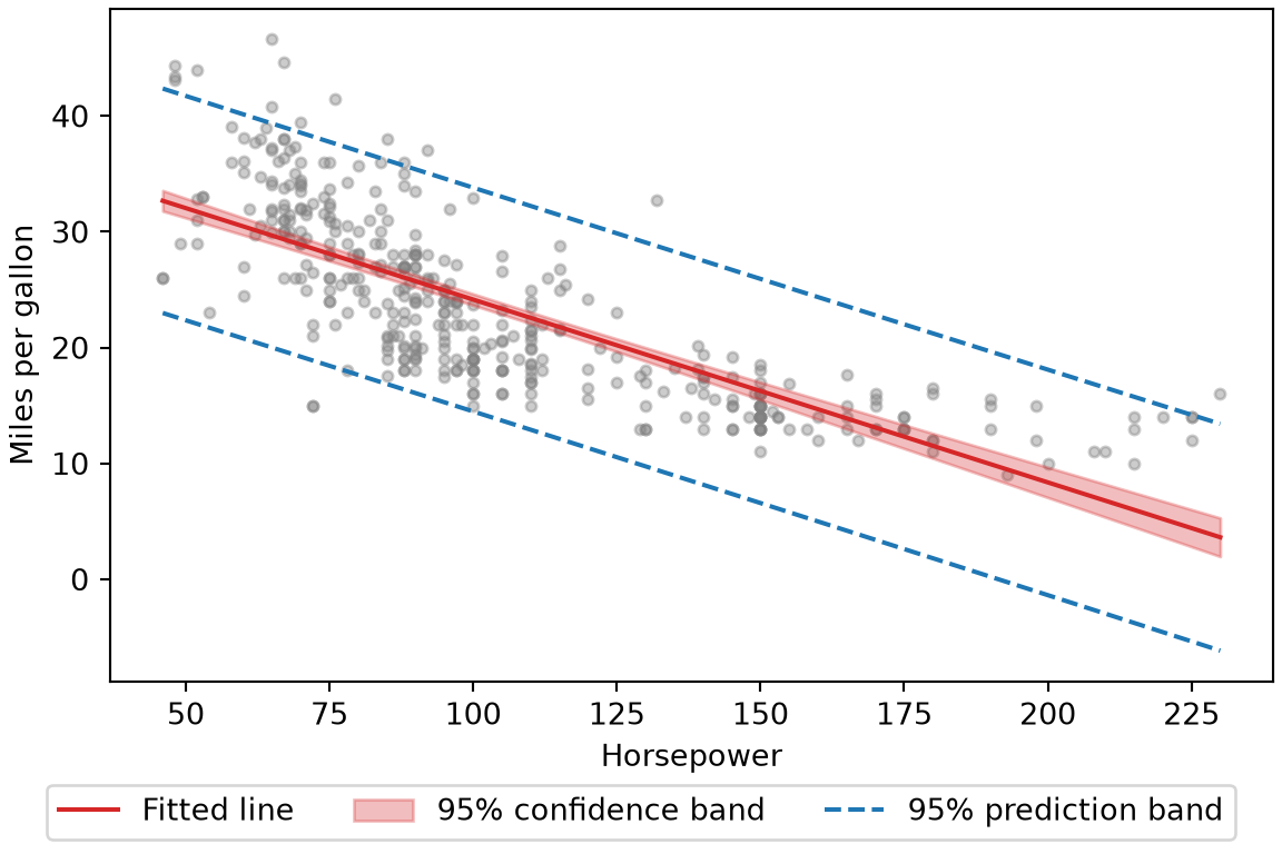
Figure 4: Fuel economy against horsepower for the Auto data, with the least squares line, its 95% confidence band for the mean response, and its 95% prediction band.
Scatter plot of miles per gallon against horsepower for 392 cars with a downward fitted line. A narrow shaded band hugs the line; it is the confidence band. Two dashed curves sit about 10 miles per gallon above and below the line; they form the prediction band, and most of the points fall between them.
predict(fit_simple, tibble::tibble(horsepower = 98), interval = "prediction")
       fit     lwr      upr
1 24.46708 14.8094 34.12476
Show code
library(ggplot2)

grid <- tibble::tibble(horsepower = seq(min(auto$horsepower),
                                    max(auto$horsepower), length.out = 100))
band_mean <- predict(fit_simple, grid, interval = "confidence")
band_pred <- predict(fit_simple, grid, interval = "prediction")
bands <- tibble::tibble(grid, fit = band_mean[, "fit"],
                    mean_lwr = band_mean[, "lwr"], mean_upr = band_mean[, "upr"],
                    pred_lwr = band_pred[, "lwr"], pred_upr = band_pred[, "upr"])
ggplot(bands, aes(horsepower)) +
  geom_point(data = auto, aes(y = mpg), colour = "grey50", alpha = 0.6) +
  geom_ribbon(aes(ymin = mean_lwr, ymax = mean_upr),
              fill = "firebrick", alpha = 0.3) +
  geom_line(aes(y = fit), colour = "firebrick") +
  geom_line(aes(y = pred_lwr), colour = "steelblue", linetype = "dashed") +
  geom_line(aes(y = pred_upr), colour = "steelblue", linetype = "dashed") +
  labs(x = "Horsepower", y = "Miles per gallon")

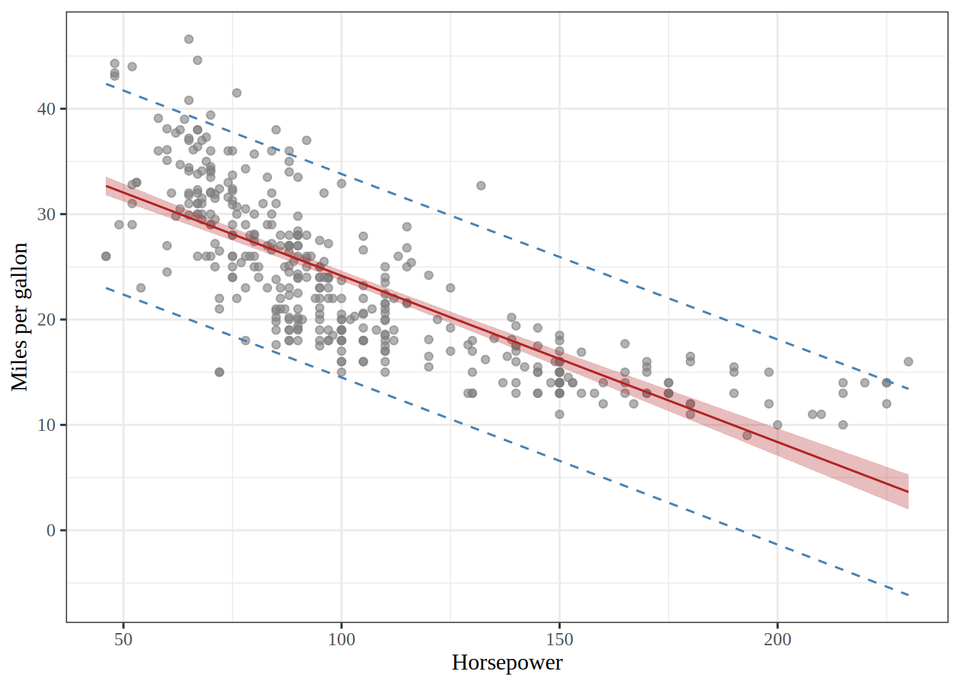
Scatter plot of miles per gallon against horsepower for 392 cars, drawn in R with ggplot2, with a downward fitted line, a narrow shaded confidence band around it, and wider dashed prediction-band curves that contain most of the points.

The prediction interval at \(98\) horsepower runs from 14.8 to 34.1 miles per gallon, about 20 times as wide as the confidence interval of Example 18. The number of cars controls the width of the confidence band, which would shrink toward the line with more data. The prediction band would not shrink below about \(\pm 2\hat\sigma\), because no amount of data removes a new car’s own noise.

LemTheorem 6 (The prediction interval is wider than the confidence interval)

Theorem 6 (The prediction interval is wider than the confidence interval) At the same input \(\vx_0\) and the same level, the prediction interval of Definition 10 is wider than the confidence interval for the mean response of Definition 9. With \(\leverage{0} = \tp{\phi_0} (\stprod{\design})^{-1} \phi_0\), the ratio of their widths is \(\sqrt{(1 + \leverage{0}) / \leverage{0}}\) [1, Sec. 3.2.2], p. 90.

Proof. Both intervals have the center \(\hat{y}_0\) and use the same \(t_{n-p^*}(0.975)\) and \(\hat\sigma\). Their half-widths are

\[ t_{n-p^*}(0.975) \, \hat\sigma \sqrt{\leverage{0}} \quad \text{and} \quad t_{n-p^*}(0.975) \, \hat\sigma \sqrt{1 + \leverage{0}}. \]

Because \(1 + \leverage{0} > \leverage{0}\), the second is larger. The ratio of the two is \(\sqrt{(1 + \leverage{0}) / \leverage{0}}\). The extra \(1\) is the variance of the new response’s own noise.

ExmExample 20 (Both intervals at every car)

Example 20 (Both intervals at every car) For each car of the Auto data, take its own horsepower as \(\vx_0\). Compute the width of the confidence interval for the mean response and of the prediction interval, and check that the prediction interval is wider at every car, with the width ratio of Theorem 6:

# Phi_simple, PtP_inv, sigma_simple and t_crit come from the examples earlier in this chapter.
h_cars = np.sum(Phi_simple @ PtP_inv * Phi_simple, axis=1)
width_mean = 2 * t_crit * sigma_simple * np.sqrt(h_cars)
width_pred = 2 * t_crit * sigma_simple * np.sqrt(1 + h_cars)
ratio_cars = width_pred / width_mean
print(np.all(width_pred > width_mean), ratio_cars.min(), ratio_cars.max())
True 5.883031030489702 19.82234421472044
conf_cars <- predict(fit_simple, auto, interval = "confidence")
pred_cars <- predict(fit_simple, auto, interval = "prediction")
width_conf <- conf_cars[, "upr"] - conf_cars[, "lwr"]
width_pred <- pred_cars[, "upr"] - pred_cars[, "lwr"]
c(all_wider = all(width_pred > width_conf),
  min_ratio = min(width_pred / width_conf),
  max_ratio = max(width_pred / width_conf))
all_wider min_ratio max_ratio 
 1.000000  5.883031 19.822344 

The prediction interval is wider than the confidence interval at 392 of the 392 cars. The ratio of widths runs from 5.9 to 19.8. It is smallest where \(\leverage{0}\) is largest, at the extreme horsepower values, where the fitted line is least certain. Even there, the new car’s own noise makes the prediction interval wider.

4 Checking the model

This section follows the list of potential problems in [1, Sec. 3.3.3]. The rme notes on diagnostics go further, with quantile-quantile (QQ) plots, Cook’s distance and formal tests.

4.1 Non-linearity

ExrExercise 13 (Plot the residuals)

Exercise 13 (Plot the residuals) For the one-feature fit, plot each car’s residual \(e_i = y_i - \hat{y}_i\) against its fitted value \(\hat{y}_i\).

Solution 13.

Show code
# A function, so the plotting calls' return values are not printed.
def plot_residuals(beta_hat, Phi, label):
    fitted_values = Phi @ beta_hat
    fig, ax = plt.subplots(figsize=(6, 4), layout="constrained")
    ax.scatter(fitted_values, y - fitted_values, s=12, alpha=0.5);
    ax.axhline(0, color="grey", linewidth=1);
    ax.set_xlabel(f"Fitted mpg ({label})");
    ax.set_ylabel("Residual");
    plt.show()

plot_residuals(beta_simple, Phi_simple, "straight line")
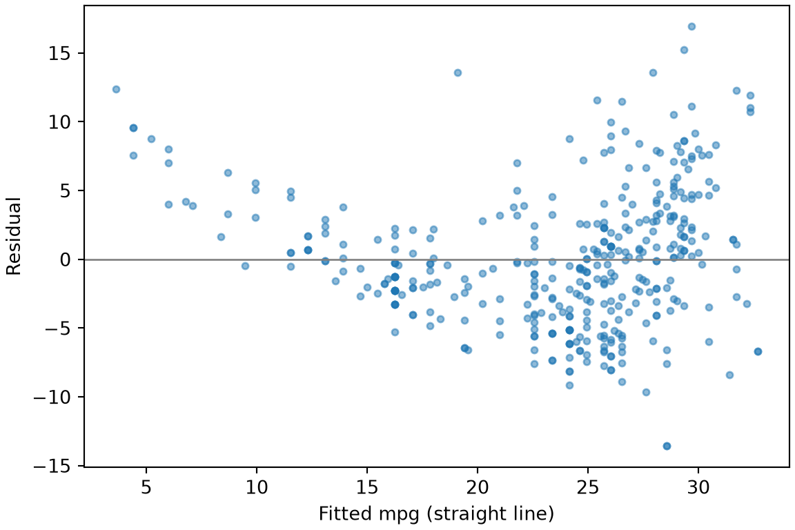
Figure 5: Residuals against fitted values for the straight-line fit of mpg on horsepower.
Scatter plot of residuals against fitted miles per gallon for 392 cars. The points form a U shape: residuals are mostly positive at low and high fitted values and mostly negative in the middle. A horizontal line marks zero.
Show code
performance::check_model(fit_simple, check = "linearity") |>
  plot()

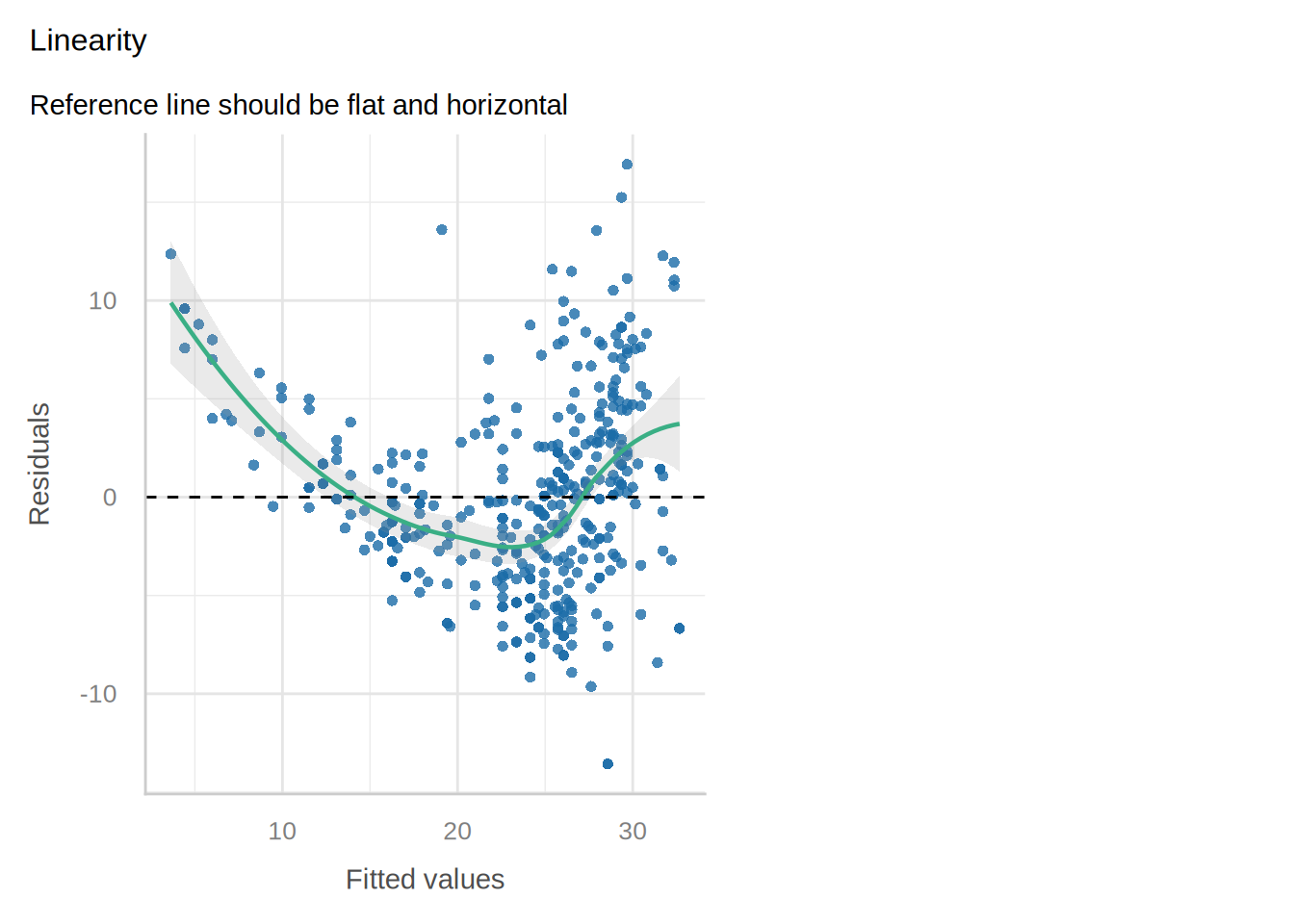
Scatter plot of residuals against fitted miles per gallon for 392 cars, drawn in R with the performance package. The points form a U shape around a dashed line at zero, and a smooth trend curve traces the U.

ExrExercise 14 (Plot the residuals (part 2))

Exercise 14 (Plot the residuals (part 2)) Use the setup of Exercise 13.

If the straight line captured the relationship, what would the plot look like?

Solution 14. If the line captured the relationship, the residuals would scatter evenly above and below \(0\) at every fitted value, with no pattern.

ExrExercise 15 (Plot the residuals (part 3))

Exercise 15 (Plot the residuals (part 3)) Use the setup of Exercise 13.

What do you see instead?

Solution 15. Instead they form a U: mostly positive at both ends and mostly negative in the middle. The line is too high in the middle of the horsepower range and too low at both ends, so the relationship is curved [1, Sec. 3.3.3], pp. 100–101.

DefDefinition 11 (Residual plot)

Definition 11 (Residual plot) A residual plot shows the residuals \(e_i = y_i - \hat{y}_i\) against the fitted values \(\hat{y}_i\) (or, in simple linear regression, against the feature). For a model that captures the relationship, the points scatter around \(0\) with no visible pattern; a curve in the plot is a sign of non-linearity [1, Sec. 3.3.3], p. 101.

ExmExample 21 (The residual plot after adding \(\text{horsepower}^2\))

Example 21 (The residual plot after adding \(\text{horsepower}^2\)) The residual plot for the quadratic fit:

Show code
plot_residuals(beta_quadratic, Phi_quadratic, "quadratic")
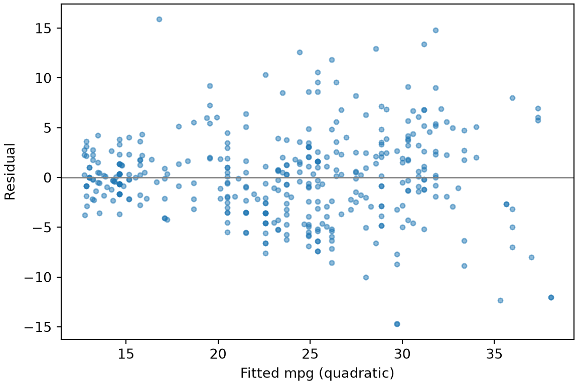
Figure 6: Residuals against fitted values for the quadratic fit of mpg on horsepower.
Scatter plot of residuals against fitted miles per gallon for the quadratic fit. The U shape is gone and the points scatter around zero, but their vertical spread grows from left to right, like a funnel opening to the right.
Show code
performance::check_model(fit_quadratic, check = "linearity") |>
  plot()

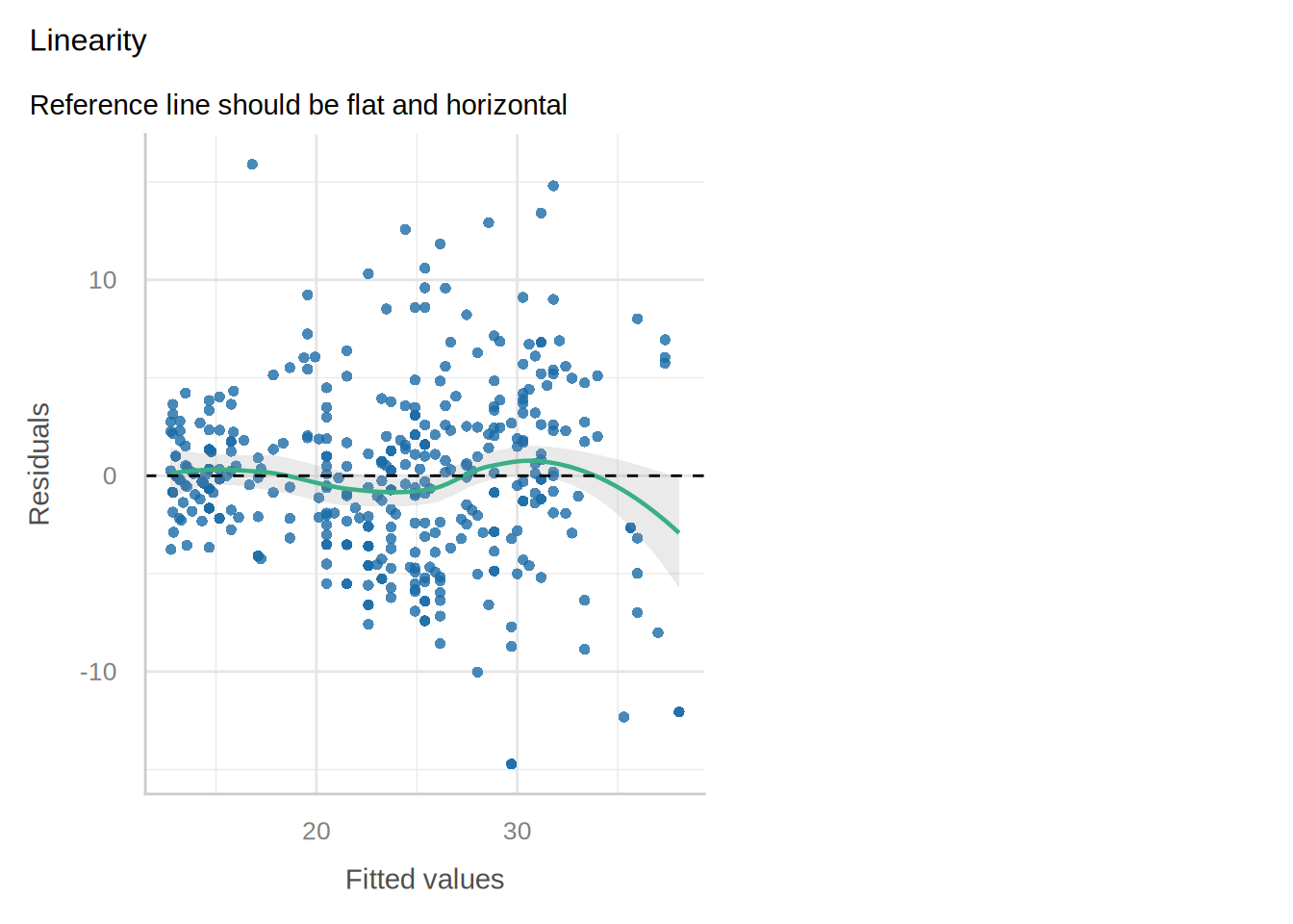
Scatter plot of residuals against fitted miles per gallon for the quadratic fit, drawn in R with the performance package. The points scatter around zero with no U shape, the smooth trend curve stays near zero, and the points spread more widely at higher fitted values.

The U shape is gone, so the quadratic term captured the curve.

4.2 Non-constant variance

ExrExercise 16 (Does the spread change?)

Exercise 16 (Does the spread change?) In the residual plot of Example 21, split the cars into thirds by fitted value, and compute the standard deviation of the residuals in each third.

Solution 16.

def spread_by_third(fitted_values, residuals):
    """Standard deviation of the residuals in each third of the fitted values."""
    cuts = np.quantile(fitted_values, [1 / 3, 2 / 3])
    third = np.searchsorted(cuts, fitted_values)
    return np.array([np.std(residuals[third == k], ddof=1) for k in range(3)])

fitted_quadratic = Phi_quadratic @ beta_quadratic
spread_quadratic = spread_by_third(fitted_quadratic, y - fitted_quadratic)
print(spread_quadratic)
[2.85532811 4.46613435 5.36238522]
# The spreads have no simple interval, so resample the cars.
# Each resample refits the quadratic, finds its own thirds, and recomputes the spreads.
def bootstrap_spread_ci(B=2000, seed=571):
    """95% percentile intervals for the three spreads and for the highest third's spread over the lowest's."""
    rng = np.random.default_rng(seed)
    spreads = np.empty((B, 3))
    for b in range(B):
        rows = rng.integers(0, n, n)
        beta_b = np.linalg.lstsq(Phi_quadratic[rows], y[rows], rcond=None)[0]
        fitted_b = Phi_quadratic[rows] @ beta_b
        spreads[b] = spread_by_third(fitted_b, y[rows] - fitted_b)
    return (np.quantile(spreads, [0.025, 0.975], axis=0),
            np.quantile(spreads[:, 2] / spreads[:, 0], [0.025, 0.975]))

spread_ci_quadratic, spread_ratio_ci = bootstrap_spread_ci()
print(spread_ci_quadratic.T)
[[2.25359029 3.54058612]
 [3.74873411 5.05624762]
 [4.56392342 6.10287934]]
print(spread_quadratic[2] / spread_quadratic[0], spread_ratio_ci)
1.878027678194057 [1.42727074 2.46554721]
spread_of_thirds <- function(fitted_values, residuals) {
  third <- cut(fitted_values, quantile(fitted_values, c(0, 1 / 3, 2 / 3, 1)),
               include.lowest = TRUE)
  tapply(residuals, third, sd)
}
spread_by_third <- function(model) {
  spread_of_thirds(fitted(model), residuals(model))
}
spread_quadratic_r <- spread_by_third(fit_quadratic)
spread_quadratic_r
[12.7,20.5] (20.5,26.4] (26.4,38.1] 
   2.855328    4.466134    5.362385 
# The spreads have no simple interval, so resample the cars.
# Each resample refits the quadratic,
# finds its own thirds, and recomputes the spreads.
boot_spread_ci <- function(model, data, n_boot = 2000) {
  set.seed(571)
  design <- model.matrix(model)
  y <- data$mpg
  spreads <- vapply(seq_len(n_boot), \(b) {
    rows <- sample(nrow(design), replace = TRUE)
    residuals_b <- lm.fit(design[rows, ], y[rows])$residuals
    spread_of_thirds(y[rows] - residuals_b, residuals_b)
  }, numeric(3))
  list(spreads = apply(spreads, 1, quantile, probs = c(0.025, 0.975)),
       ratio = quantile(spreads[3, ] / spreads[1, ], c(0.025, 0.975)))
}
spread_ci_r <- boot_spread_ci(fit_quadratic, auto)
t(spread_ci_r$spreads)
                2.5%    97.5%
[13.5,22.4] 2.260491 3.576468
(22.4,26.9] 3.706911 5.048198
(26.9,36.7] 4.588323 6.087379
spread_quadratic_r[[3]] / spread_quadratic_r[[1]]
[1] 1.878028
spread_ci_r$ratio
    2.5%    97.5% 
1.418753 2.458572 
ExrExercise 17 (Does the spread change? (part 2))

Exercise 17 (Does the spread change? (part 2)) Use the setup of Exercise 16.

Is the spread of the residuals the same across the range of fitted values?

Solution 17. No. The standard deviation grows from 2.9 (95% bootstrap interval 2.3 to 3.5) in the lowest third to 5.4 (4.6 to 6.1) in the highest, so the plot fans out like a funnel. The highest third’s spread is 1.9 times the lowest third’s (1.4 to 2.5), an interval that excludes \(1\), the ratio for equal spreads. Each interval is the 2.5th to 97.5th percentile over 2,000 resamples of the cars, refitting the quadratic and recomputing the thirds each time.

ExrExercise 18 (Does the spread change? (part 3))

Exercise 18 (Does the spread change? (part 3)) Use the setup of Exercise 16.

Which assumption of Theorem 1 does that bear on?

Solution 18. Theorem 1 assumes \(\Cov{\veps} = \sigma^2 \mathbf{I}_n\), the same variance \(\sigma^2\) for every car. A funnel says the noise variance grows with the fitted value, which pds calls heteroskedasticity. Then the standard errors estimated as in Definition 4, and the intervals and tests built on them, are no longer right [1, Sec. 3.3.3], p. 103.

ExmExample 22 (Fitting \(\log(\text{mpg})\) instead)

Example 22 (Fitting \(\log(\text{mpg})\) instead) A common remedy for a funnel is to model a concave function of the response, such as \(\log y\), which shrinks large responses more than small ones [1, Sec. 3.3.3], p. 103. Refit the quadratic model with \(\log(\text{mpg})\) as the response, and repeat Exercise 16:

log_y = np.log(y)
beta_log = np.linalg.lstsq(Phi_quadratic, log_y, rcond=None)[0]
fitted_log = Phi_quadratic @ beta_log
spread_log = spread_by_third(fitted_log, log_y - fitted_log)
print(spread_log)
[0.15802602 0.18322063 0.18559353]
print(spread_quadratic[2] / spread_quadratic[0], spread_log[2] / spread_log[0])
1.878027678194057 1.1744492221667266
# Bootstrap: resample cars, refit the quadratic model to each response,
# and recompute the ratio of the highest third's spread to the lowest third's.
rng_log = np.random.default_rng(571)
ratio_boot = np.empty((2000, 2))
for b in range(2000):
    rows = rng_log.integers(0, n, n)
    for j, response in enumerate([y, log_y]):
        beta_b = np.linalg.lstsq(Phi_quadratic[rows], response[rows], rcond=None)[0]
        fitted_b = Phi_quadratic[rows] @ beta_b
        spread_b = spread_by_third(fitted_b, response[rows] - fitted_b)
        ratio_boot[b, j] = spread_b[2] / spread_b[0]
# Columns: original scale, log scale; rows: 2.5th and 97.5th percentiles.
ratio_ci = np.quantile(ratio_boot, [0.025, 0.975], axis=0)
print(ratio_ci)
[[1.42727074 0.93581492]
 [2.46554721 1.4846279 ]]
fit_log <- lm(log(mpg) ~ horsepower + I(horsepower^2), data = auto)
spread_by_third(fit_log)
[2.53,2.99] (2.99,3.24]  (3.24,3.7] 
  0.1580260   0.1832206   0.1855935 
# Bootstrap: resample cars, refit the quadratic model to each response,
# and recompute the ratio of the highest third's spread to the lowest third's.
set.seed(571)
ratio_boot <- replicate(2000, {
  boot_cars <- auto[sample(nrow(auto), replace = TRUE), ]
  spread_orig <- spread_by_third(
    lm(mpg ~ horsepower + I(horsepower^2), data = boot_cars))
  spread_log <- spread_by_third(
    lm(log(mpg) ~ horsepower + I(horsepower^2), data = boot_cars))
  c(original = spread_orig[[3]] / spread_orig[[1]],
    log = spread_log[[3]] / spread_log[[1]])
})
# Rows: 2.5th and 97.5th percentiles; columns: original scale, log scale.
apply(ratio_boot, 1, quantile, c(0.025, 0.975))
      original      log
2.5%  1.418753 0.931214
97.5% 2.458572 1.467118

On the original scale, the highest third’s residual spread was 1.88 times the lowest third’s, with a \(95\%\) bootstrap percentile interval from 1.43 to 2.47. On the log scale, the ratio is 1.17, with an interval from 0.94 to 1.48. Equal spread in the two thirds is a ratio of \(1\): the original-scale interval excludes it, and the log-scale interval includes it. Each interval comes from \(2000\) resamples of the cars, refitting the model each time, and describes which cars were drawn. Another remedy, when the variance of each response is known up to a constant, is weighted least squares, which gives each squared residual a weight inversely proportional to that response’s variance [1, Sec. 3.3.3], p. 103.

4.3 Correlated errors

ExrExercise 19 (Plot the residuals in time order)

Exercise 19 (Plot the residuals in time order) The rows of the Auto data are sorted by model year. For the quadratic fit, compute the correlation between each residual and the next one in the file, and the average residual for each model year. Theorem 1 assumes the noise terms are uncorrelated. Do the residuals look uncorrelated?

Solution 19.

def lag_correlation(residuals):
    """Correlation between each residual and the next one in the file."""
    return np.corrcoef(residuals[:-1], residuals[1:])[0, 1]

residuals_quadratic = y - fitted_quadratic
lag_quadratic = lag_correlation(residuals_quadratic)
year_means = pd.Series(residuals_quadratic).groupby(year).mean()
year_means_min, year_means_max = year_means.min(), year_means.max()
last_negative_year = int(year_means.index[year_means < 0].max())
print(lag_quadratic)
0.4602676830246073
print(year_means)
70.0   -0.616227
71.0   -1.750040
72.0   -1.938788
73.0   -2.506749
74.0   -2.170697
75.0   -2.926681
76.0   -2.024674
77.0    0.326999
78.0    0.439857
79.0    1.808373
80.0    5.245947
81.0    2.593976
82.0    4.701654
dtype: float64
# Each year's average residual, with a 95% t interval from the cars of that year
residuals_by_year = pd.Series(residuals_quadratic).groupby(year)
year_table = pd.DataFrame({"mean": residuals_by_year.mean(),
                           "sem": residuals_by_year.sem(),
                           "df": residuals_by_year.count() - 1})
year_table["half"] = stats.t.ppf(0.975, year_table["df"]) * year_table["sem"]
year_table["lower"] = year_table["mean"] - year_table["half"]
year_table["upper"] = year_table["mean"] + year_table["half"]
year_table["year"] = year_table.index.astype(int)
print(year_table[["year", "mean", "lower", "upper"]].to_string(index=False))
 year      mean     lower     upper
   70 -0.616227 -1.903516  0.671061
   71 -1.750040 -3.100018 -0.400061
   72 -1.938788 -3.191400 -0.686177
   73 -2.506749 -3.560732 -1.452767
   74 -2.170697 -3.193823 -1.147571
   75 -2.926681 -4.515174 -1.338188
   76 -2.024674 -3.075580 -0.973768
   77  0.326999 -0.683219  1.337218
   78  0.439857 -0.710148  1.589862
   79  1.808373  0.316701  3.300046
   80  5.245947  3.100536  7.391358
   81  2.593976  1.185572  4.002381
   82  4.701654  3.459409  5.943899
beta_with_year, Phi_with_year = fit([horsepower, horsepower ** 2, year])
lag_with_year = lag_correlation(y - Phi_with_year @ beta_with_year)
print(lag_with_year)
0.3075231574213514
# Neighboring residuals are correlated, so resampling single cars would break the order.
# Instead resample blocks of 20 consecutive cars, refit the model, and recompute the correlation.
def block_bootstrap_lag_ci(Phi, block=20, B=20000, seed=571):
    """95% percentile interval for the neighboring-residual correlation from resampled blocks of cars."""
    rng = np.random.default_rng(seed)
    n_blocks = int(np.ceil(n / block))
    lag = np.empty(B)
    for b in range(B):
        starts = rng.integers(0, n - block + 1, n_blocks)
        rows = (starts[:, None] + np.arange(block)).ravel()[:n]
        beta_b = np.linalg.lstsq(Phi[rows], y[rows], rcond=None)[0]
        lag[b] = lag_correlation(y[rows] - Phi[rows] @ beta_b)
    return np.quantile(lag, [0.025, 0.975])

lag_ci_quadratic = block_bootstrap_lag_ci(Phi_quadratic)
lag_ci_with_year = block_bootstrap_lag_ci(Phi_with_year)
print(lag_ci_quadratic, lag_ci_with_year)
[0.31733878 0.50875017] [0.1433561  0.38124989]
lag_correlation <- function(e) cor(head(e, -1), tail(e, -1))
lag_correlation(residuals(fit_quadratic))
[1] 0.4602677
tapply(residuals(fit_quadratic), auto$year, mean)
        70         71         72         73         74         75         76 
-0.6162271 -1.7500396 -1.9387883 -2.5067494 -2.1706968 -2.9266811 -2.0246741 
        77         78         79         80         81         82 
 0.3269993  0.4398570  1.8083732  5.2459472  2.5939761  4.7016539 
# Each year's average residual,
# with a 95% t interval from the cars of that year
sapply(split(residuals(fit_quadratic), auto$year), function(e) {
  half <- qt(0.975, length(e) - 1) * sd(e) / sqrt(length(e))
  c(mean = mean(e), lower = mean(e) - half, upper = mean(e) + half)
}) |>
  t()
         mean      lower      upper
70 -0.6162271 -1.9035155  0.6710612
71 -1.7500396 -3.1000185 -0.4000607
72 -1.9387883 -3.1914000 -0.6861766
73 -2.5067494 -3.5607316 -1.4527671
74 -2.1706968 -3.1938231 -1.1475706
75 -2.9266811 -4.5151741 -1.3381881
76 -2.0246741 -3.0755802 -0.9737680
77  0.3269993 -0.6832193  1.3372179
78  0.4398570 -0.7101477  1.5898617
79  1.8083732  0.3167006  3.3000458
80  5.2459472  3.1005363  7.3913580
81  2.5939761  1.1855717  4.0023805
82  4.7016539  3.4594092  5.9438985
fit_with_year <- lm(mpg ~ horsepower + I(horsepower^2) + year, data = auto)
lag_correlation(residuals(fit_with_year))
[1] 0.3075232
# Neighboring residuals are correlated,
# so resampling single cars would break the order.
# Instead resample blocks of 20 consecutive cars,
# refit the model, and recompute the correlation.
block_bootstrap_lag_ci <- function(model, block = 20, n_boot = 20000) {
  set.seed(571)
  design <- model.matrix(model)
  y <- model.response(model.frame(model))
  n_blocks <- ceiling(nrow(design) / block)
  lag <- vapply(seq_len(n_boot), \(b) {
    starts <- sample(nrow(design) - block + 1, n_blocks, replace = TRUE)
    rows <- head(as.vector(outer(0:(block - 1), starts, "+")), nrow(design))
    lag_correlation(lm.fit(design[rows, ], y[rows])$residuals)
  }, numeric(1))
  unname(quantile(lag, c(0.025, 0.975)))
}
block_bootstrap_lag_ci(fit_quadratic)
[1] 0.3175578 0.5078073
block_bootstrap_lag_ci(fit_with_year)
[1] 0.1445910 0.3820917
Show code
year_table_py <- py$year_table
year_min <- year_table_py[which.min(year_table_py$mean), ]
year_max <- year_table_py[which.max(year_table_py$mean), ]

No. Neighboring residuals have correlation 0.46 (95% bootstrap interval 0.32 to 0.51). The interval comes from 20,000 resamples of blocks of \(20\) consecutive cars, which keep the order of the file, with the quadratic refitted and the correlation recomputed on each resample. The average residual is negative for every year up to 1976 and positive for every later year (Figure 7), ranging from -2.9 (1975, 95% interval -4.5 to -1.3) to 5.2 (1980, 3.1 to 7.4): the model over-predicts the older cars and under-predicts the newer ones. Each year’s interval is a 95% \(t\) interval for the average residual of the cars of that year, and it excludes \(0\) in 10 of the 13 years. James et al. [1, Sec. 3.3.3], p. 102 calls runs of same-signed neighboring residuals tracking. With correlated errors, the estimated standard errors of Definition 4 are too small, and the confidence intervals too narrow [1, Sec. 3.3.3], p. 101.

Figure 7: The average residual of the quadratic fit for each year, with each year’s 95% \(t\) interval.

Part of the cause is a missing feature. Adding year to the model lowers the neighboring correlation to 0.31 (0.14 to 0.38), but does not remove it.

4.4 Outliers

DefDefinition 12 (Standardized residual)

Definition 12 (Standardized residual) The standardized residual of observation \(i\) is its residual divided by its estimated standard deviation,

\[ r_i = \frac{e_i}{\hat\sigma \sqrt{1 - \leverage{i}}}, \]

where \(\leverage{i}\) is the leverage and \(\hat\sigma\) is the residual standard error. Dividing by \(\sqrt{1 - \leverage{i}}\) accounts for high-leverage points having smaller residuals, because they pull the fit toward themselves.

ExmExample 23 (Standardized residuals of the quadratic fit)

Example 23 (Standardized residuals of the quadratic fit) Compute the standardized residuals of the quadratic fit, and look at the car with the highest leverage:

PtP_inv_quadratic = np.linalg.inv(Phi_quadratic.T @ Phi_quadratic)
h_quadratic = np.sum(Phi_quadratic @ PtP_inv_quadratic * Phi_quadratic, axis=1)
sigma_quadratic = np.sqrt(np.sum(residuals_quadratic ** 2) / (n - 3))
r_quadratic = residuals_quadratic / (sigma_quadratic * np.sqrt(1 - h_quadratic))
top_leverage = np.argmax(h_quadratic)
print(Auto.loc[top_leverage, ["name", "horsepower", "mpg"]])
name          pontiac grand prix
horsepower                   230
mpg                         16.0
Name: 115, dtype: object
print(h_quadratic[top_leverage], residuals_quadratic[top_leverage],
      r_quadratic[top_leverage])
0.09359709306399572 1.2281554548362656 0.2949319391422815
r_quadratic <- rstandard(fit_quadratic)
top_leverage <- which.max(hatvalues(fit_quadratic))
auto |>
  dplyr::mutate(id = dplyr::row_number()) |>
  dplyr::filter(id == top_leverage) |>
  dplyr::select(id, name, horsepower, mpg)
c(leverage = hatvalues(fit_quadratic)[[top_leverage]],
  residual = residuals(fit_quadratic)[[top_leverage]],
  standardized = r_quadratic[[top_leverage]])
    leverage     residual standardized 
  0.09359709   1.22815545   0.29493194 

The car with the highest leverage has \(\leverage{i} =\) 0.094, residual \(e_i =\) 1.23 and standardized residual \(r_i =\) 0.29. R’s rstandard() gives the same \(r_i\) for every car: the largest difference from the Python values is \(4\times 10^{-13}\), which is rounding error.

NoteOther names for standardized residuals

James et al. [1, Sec. 3.3.3], p. 104 calls \(r_i\) a studentized residual, and R computes it with rstandard(). Other sources keep studentized for the version that estimates \(\sigma\) without observation \(i\), which R computes with rstudent(). These notes say standardized.

DefDefinition 13 (Outlier)

Definition 13 (Outlier) An outlier is an observation whose response is far from what the model predicts. A common rule of thumb flags observation \(i\) as a possible outlier when its standardized residual (Definition 12) has \(|r_i| > 3\) [1, Sec. 3.3.3], p. 104.

ExmExample 24 (Outliers in the quadratic fit)

Example 24 (Outliers in the quadratic fit) List the cars whose standardized residuals in Example 23 have \(|r_i| > 3\):

outliers = np.abs(r_quadratic) > 3
print(Auto.loc[outliers, ["name", "horsepower", "mpg"]].assign(r=r_quadratic[outliers]))
                    name  horsepower   mpg         r
152      mercury monarch          72  15.0 -3.372439
153        ford maverick          72  15.0 -3.372439
320            mazda glc          65  46.6  3.397282
327  honda civic 1500 gl          67  44.6  3.076382
330        datsun 280-zx         132  32.7  3.646286
auto |>
  dplyr::mutate(id = dplyr::row_number(), r = r_quadratic) |>
  dplyr::filter(abs(r) > 3) |>
  dplyr::select(id, name, horsepower, mpg, r)

5 of the \(392\) cars have \(|r_i| > 3\), and the largest is \(|r_i| =\) 3.65. Of these, 3 get more miles per gallon than the model predicts, and 2 get fewer. Under Gaussian noise with constant variance, about 1.1 of \(392\) cars would have \(|r_i| > 3\) by chance, so there are more than chance alone would give. Before removing an outlier, check whether it is a recording error; if it is not, it may be a sign that the model is missing something, such as a feature [1, Sec. 3.3.3], p. 104.

4.5 High-leverage points

ExmExample 25 (The highest-leverage car)

Example 25 (The highest-leverage car) The leverage \(\leverage{i}\) measures how unusual car \(i\)’s features are. Its average is \(p^*/n\), and James et al. [1, Sec. 3.3.3], p. 106 flags points whose leverage greatly exceeds that average. Find the highest-leverage car in the one-feature fit:

h_simple = np.sum(Phi_simple @ PtP_inv * Phi_simple, axis=1)
top = np.argmax(h_simple)
print(Auto.loc[top, ["name", "horsepower"]], h_simple[top], 2 / n)
name          pontiac grand prix
horsepower                   230
Name: 115, dtype: object 0.02975300179092146 0.00510204081632653
h_simple <- hatvalues(fit_simple)
auto |>
  dplyr::mutate(id = dplyr::row_number()) |>
  dplyr::filter(id == which.max(h_simple)) |>
  dplyr::select(id, name, horsepower)
c(max = max(h_simple), average = mean(h_simple))
        max     average 
0.029753002 0.005102041 

The pontiac grand prix, with 230 horsepower, has leverage 0.0298, about 5.8 times the average \(2/392\). Its horsepower is the largest in the data, far from the sample mean of 104. A high-leverage point is worth checking: since \(\hat{\vy} = \hatmat\vy\), a change in its response moves its own fitted value by \(\leverage{i}\) times that change, more than the same change would for any other car.

4.6 Collinearity

DefDefinition 14 (Variance inflation factor)

Definition 14 (Variance inflation factor) Let \(\design\) have an intercept column and \(p\) features \(x_1, \dots, x_p\), and let \(R^2_j\) be the coefficient of determination of the regression of feature \(x_j\) on the other \(p - 1\) features (with an intercept). The variance inflation factor (VIF) [5] of feature \(x_j\) is

\[ \operatorname{VIF}_j \eqdef \frac{1}{1 - R^2_j}. \]

It is at least \(1\), and equals \(1\) exactly when the other features cannot predict \(x_j\) at all, in the sample (\(R^2_j = 0\)). It grows without bound as \(x_j\) approaches a linear combination of the other features (\(R^2_j \to 1\)).

ExmExample 26 (Collinearity of horsepower and weight)

Example 26 (Collinearity of horsepower and weight) Definition 14 defines the variance inflation factor, \(\operatorname{VIF}_j = 1 / (1 - R^2_j)\). Compute it for horsepower and weight in the two-feature fit:

r_hp_weight = np.corrcoef(horsepower, weight)[0, 1]
vif_hp_weight = 1 / (1 - r_hp_weight ** 2)
print(vif_hp_weight)
3.959227866518292
# Bootstrap: resample cars with replacement and recompute the VIF each time.
rng_vif = np.random.default_rng(571)
vif_boot = np.empty(2000)
for b in range(2000):
    rows = rng_vif.integers(0, len(horsepower), len(horsepower))
    r_boot = np.corrcoef(horsepower[rows], weight[rows])[0, 1]
    vif_boot[b] = 1 / (1 - r_boot ** 2)
# The 2.5th and 97.5th percentiles of the resampled VIFs.
vif_ci = np.quantile(vif_boot, [0.025, 0.975])
print(vif_ci)
[3.28696834 4.78555867]
r2_hp <- summary(lm(horsepower ~ weight, data = auto))$r.squared
1 / (1 - r2_hp)
[1] 3.959228
# Bootstrap: resample cars with replacement and recompute the VIF each time.
set.seed(571)
vif_boot <- replicate(2000, {
  rows <- sample(nrow(auto), replace = TRUE)
  1 / (1 - cor(auto$horsepower[rows], auto$weight[rows])^2)
})
# The 2.5th and 97.5th percentiles of the resampled VIFs.
quantile(vif_boot, c(0.025, 0.975))
    2.5%    97.5% 
3.267544 4.794859 

With only two features, \(R^2_j\) is the squared correlation, so both features have the same VIF, 3.96. The variance of each coefficient is 3.96 times what it would be if the two features were uncorrelated. A \(95\%\) bootstrap percentile interval for the VIF, from \(2000\) resamples of the cars, runs from 3.29 to 4.79. The bootstrap fits here because the VIF is a nonlinear function of the correlation, and the interval describes which cars were drawn. The interval lies entirely below the common warning level of \(5\) to \(10\) [1, Sec. 3.3.3], p. 108, and the VIF explains why the horsepower standard error grows from 0.0064 in the one-feature fit to 0.011 in Example 13.

RemarkRemark 2 (Variance inflation from collinear features)

Remark 2 (Variance inflation from collinear features). In a model with an intercept, the variance of the least squares estimate of the coefficient of feature \(x_j\) is

\[ \Var{\hb_j} = \frac{\sigma^2}{(n-1) s_{x_j}^2} \operatorname{VIF}_j, \]

where \(\sigma^2\) is the error variance and \(s_{x_j}^2\) is the sample variance of \(x_j\). The formula follows from the covariance of the least squares estimate (Theorem 1), and James et al. [1, Sec. 3.3.3] defines the VIF. The factor \(\sigma^2 / ((n-1) s_{x_j}^2)\) is the variance of the slope in a simple linear regression on \(x_j\) alone, so \(\operatorname{VIF}_j\) (Definition 14) is the factor by which the other features inflate the variance of \(\hb_j\). Features that are nearly collinear, such as the powers of one feature in the remark on stability of expansions, have large VIFs and imprecise coefficients.

5 Choosing features

Adapted from [1, Sec. 3.2.1].

The features that a model keeps change the meaning of each of its coefficients. The chapter Subset Selection covers ways to choose the features, such as forward selection.

5.1 A coefficient depends on the other features

ExrExercise 20 (Does faster acceleration raise fuel economy?)

Exercise 20 (Does faster acceleration raise fuel economy?) In the Auto data, acceleration is the time in seconds a car takes to go from 0 to 60 miles per hour, so a larger value means a slower car.

Fit mpg on acceleration alone.

Solution 20.

acceleration = Auto["acceleration"].to_numpy(float)
beta_acc, Phi_acc = fit([acceleration])
# Each coefficient with its 95% confidence interval
print(np.column_stack([beta_acc, coef_ci(beta_acc, Phi_acc)]))
[[4.8332498  0.80576513 8.86073448]
 [1.19762419 0.94245663 1.45279175]]
# The table includes each coefficient's 95% confidence interval
lm(mpg ~ acceleration, data = auto) |>
  parameters::parameters() |>
  parameters::print_md(digits = 3)
Parameter Coefficient SE 95% CI t(390) p
(Intercept) 4.833 2.048 (0.806, 8.861) 2.359 0.019
acceleration 1.198 0.130 (0.942, 1.453) 9.228 < .001
Show code
coef_ci_acc <- py$coef_ci(py$beta_acc, py$Phi_acc)
ExrExercise 21 (Does faster acceleration raise fuel economy? (part 2))

Exercise 21 (Does faster acceleration raise fuel economy? (part 2)) Use the setup of Exercise 20.

What is the sign of the slope?

Solution 21. On its own, acceleration has slope 1.198, so slower cars get more miles per gallon.

ExrExercise 22 (Does faster acceleration raise fuel economy? (part 3))

Exercise 22 (Does faster acceleration raise fuel economy? (part 3)) Use the setup of Exercise 20.

Is it significant?

Solution 22. The 95% confidence interval for the slope is 0.942 to 1.453, and \(p = 1.8\times10^{-18}\), so the slope is significant at the \(5\%\) level.

ExrExercise 23 (Does faster acceleration raise fuel economy? (part 4))

Exercise 23 (Does faster acceleration raise fuel economy? (part 4)) Use the setup of Exercise 20.

Add horsepower to the model. What happens to the acceleration coefficient?

Solution 23.

beta_acc_hp, Phi_acc_hp = fit([acceleration, horsepower])
# Each coefficient with its 95% confidence interval
print(np.column_stack([beta_acc_hp, coef_ci(beta_acc_hp, Phi_acc_hp)]))
[[52.55932488 47.47298392 57.64566585]
 [-0.60977221 -0.8464122  -0.37313222]
 [-0.18796643 -0.20492766 -0.17100519]]
# The table includes each coefficient's 95% confidence interval
lm(mpg ~ acceleration + horsepower, data = auto) |>
  parameters::parameters() |>
  parameters::print_md(digits = 3)
Parameter Coefficient SE 95% CI t(389) p
(Intercept) 52.559 2.587 (47.473, 57.646) 20.316 < .001
acceleration -0.610 0.120 (-0.846, -0.373) -5.066 < .001
horsepower -0.188 0.009 (-0.205, -0.171) -21.788 < .001
Show code
coef_ci_acc_hp <- py$coef_ci(py$beta_acc_hp, py$Phi_acc_hp)

With horsepower in the model, the acceleration coefficient is -0.610 (-0.846 to -0.373). It has changed sign. Each coefficient’s interval is its \(t\) interval, the estimate plus or minus a \(t\) quantile times its standard error.

ExrExercise 24 (Does faster acceleration raise fuel economy? (part 5))

Exercise 24 (Does faster acceleration raise fuel economy? (part 5)) Use the setup of Exercise 20.

Explain the change.

Solution 24.

print(np.corrcoef(acceleration, horsepower)[0, 1])
-0.6891955103342359
# bootstrap_corr_ci() is one of the interval helpers
corr_ci_acc_hp = bootstrap_corr_ci(acceleration, horsepower)
print(corr_ci_acc_hp)
[-0.73918546 -0.63352643]
cor(auto$acceleration, auto$horsepower)
[1] -0.6891955
# boot_cor_ci() is one of the interval helpers
boot_cor_ci(auto$acceleration, auto$horsepower)
[1] -0.7378244 -0.6332126

The two features have correlation -0.69 (95% bootstrap interval -0.74 to -0.63, from 20,000 resamples of the cars): cars with small engines are slow. In the one-feature fit, acceleration stands in for engine power, and gets the credit for the association between engine power and mpg. Holding horsepower fixed, a slower car gets fewer miles per gallon, not more. James et al. [1, Sec. 3.2.1], p. 83 calls such a feature a surrogate. Their example is a regression of shark attacks on ice cream sales at a beach: the slope is positive, because hot weather brings both, and ice cream sales are no longer significant once temperature is in the model. As in the two-feature fit, a feature’s coefficient depends on which other features are in the model.

Definitions on this page

Back to top

References

[1]
G. James, D. Witten, T. Hastie, R. Tibshirani, and J. Taylor, An introduction to statistical learning: With applications in Python. Springer, 2023. doi: 10.1007/978-3-031-38747-0.
[2]
G. James, D. Witten, T. Hastie, and R. Tibshirani, An introduction to statistical learning with applications in R, 2nd ed. Springer, 2021. Available: https://www.statlearning.com/
[3]
Wikipedia contributors, “Interaction (statistics) — Wikipedia, the free encyclopedia.” 2026. Available: https://en.wikipedia.org/wiki/Interaction_(statistics)
[4]
Wikipedia contributors, “Prediction interval — Wikipedia, the free encyclopedia.” 2026. Available: https://en.wikipedia.org/wiki/Prediction_interval
[5]
Wikipedia contributors, “Variance inflation factor — Wikipedia, the free encyclopedia.” 2026. Available: https://en.wikipedia.org/wiki/Variance_inflation_factor