Classification Lab

Published

Last modified: 2026-11-19

Show code
# The Python chunks on this page import matplotlib, pandas,
# scikit-learn and statsmodels; reticulate provisions them.
py_packages <- c("matplotlib", "pandas", "scikit-learn", "statsmodels")
library(reticulate) # nolint: undesirable_function_linter
library(tidymodels) # nolint: undesirable_function_linter
py_require(py_packages)

1 The book’s Chapter 4 lab

This page holds the code lab for the Discriminant Analysis chapter.

To work the lab without the solutions, download a stub with only the exercises:

Each solution shows the code in Python and in R.

Section 4.7 of the book [1] is the source of these exercises. The logistic regression exercises use the Smarket data, as the lab does. An exercise in the logistic regression chapter fits the model with all six predictors on the days before 2005. The discriminant analysis chapter compares this model with two other classifiers. The Python code follows the book’s Chapter 4 lab notebook, with scikit-learn [2] in place of the ISLP package. The R code uses knn from the class package, which ships with R.

2 Logistic regression on the stock market data

DatasetDataset 1: The stock market (Smarket) data
Dataset 1: The stock market (Smarket) data

Daily percentage returns of the S&P 500 stock index on 1250 trading days from 2001 to 2005 make up the Smarket data [1, Sec. 4.7]. The data are in data/smarket.csv, one row per trading day, copied from the ISLP Python package. The columns this course uses are:

  • Direction: the outcome, whether the index rose (Up) or fell (Down) that day.
  • Lag1 to Lag5: the percentage returns on each of the five previous trading days.
  • Volume: the number of shares traded on the previous day, in billions.
  • Year: the year of the trading day.

The Today column, the day’s own return, is not a predictor, because Direction is Down exactly when Today is negative.

The Date column, the calendar date of each trading day, is not used by the exercises; it names the day that a row describes, from 2001-01-10 to 2005-12-30. The ISLP copy has no dates. The dates were recovered by matching Today against the S&P 500 daily returns in the sp500ret data of the rugarch package [3], after converting those log returns to percentage returns. The script tools/add_smarket_dates.R does the match. It stops unless exactly one run of trading days agrees with all 1250 values of Today, to within 0.0005 percentage points, the rounding of Today.

Code: read the Smarket data and show it
smarket_preview <- readr::read_csv("data/smarket.csv", show_col_types = FALSE)
smarket_preview
Code: summarize each variable of the Smarket data
dim(smarket_preview)
[1] 1250   10
Code: summarize each variable of the Smarket data
skimr::skim_without_charts(smarket_preview)

Variable type: character

skim_variable n_missing complete_rate min max empty n_unique whitespace
Direction 0 1 2 4 0 2 0

Variable type: Date

skim_variable n_missing complete_rate min max median n_unique
Date 0 1 2001-01-10 2005-12-30 2003-07-10 1250

Variable type: numeric

skim_variable n_missing complete_rate mean sd p0 p25 p50 p75 p100
Year 0 1 2003.02 1.41 2001.00 2002.00 2003.00 2004.00 2005.00
Lag1 0 1 0.00 1.14 -4.92 -0.64 0.04 0.60 5.73
Lag2 0 1 0.00 1.14 -4.92 -0.64 0.04 0.60 5.73
Lag3 0 1 0.00 1.14 -4.92 -0.64 0.04 0.60 5.73
Lag4 0 1 0.00 1.14 -4.92 -0.64 0.04 0.60 5.73
Lag5 0 1 0.01 1.15 -4.92 -0.64 0.04 0.60 5.73
Volume 0 1 1.48 0.36 0.36 1.26 1.42 1.64 3.15
Today 0 1 0.00 1.14 -4.92 -0.64 0.04 0.60 5.73
Code: read the Smarket data and show it
import pandas as pd

pd.set_option("display.max_columns", None)
pd.set_option("display.width", 120)

smarket_preview = pd.read_csv("data/smarket.csv")
smarket_preview
      Year   Lag1   Lag2   Lag3   Lag4   Lag5   Volume  Today Direction        Date
0     2001  0.381 -0.192 -2.624 -1.055  5.010  1.19130  0.959        Up  2001-01-10
1     2001  0.959  0.381 -0.192 -2.624 -1.055  1.29650  1.032        Up  2001-01-11
2     2001  1.032  0.959  0.381 -0.192 -2.624  1.41120 -0.623      Down  2001-01-12
3     2001 -0.623  1.032  0.959  0.381 -0.192  1.27600  0.614        Up  2001-01-16
4     2001  0.614 -0.623  1.032  0.959  0.381  1.20570  0.213        Up  2001-01-17
...    ...    ...    ...    ...    ...    ...      ...    ...       ...         ...
1245  2005  0.422  0.252 -0.024 -0.584 -0.285  1.88850  0.043        Up  2005-12-23
1246  2005  0.043  0.422  0.252 -0.024 -0.584  1.28581 -0.955      Down  2005-12-27
1247  2005 -0.955  0.043  0.422  0.252 -0.024  1.54047  0.130        Up  2005-12-28
1248  2005  0.130 -0.955  0.043  0.422  0.252  1.42236 -0.298      Down  2005-12-29
1249  2005 -0.298  0.130 -0.955  0.043  0.422  1.38254 -0.489      Down  2005-12-30

[1250 rows x 10 columns]
Code: summarize each variable of the Smarket data
smarket_preview.info()
<class 'pandas.DataFrame'>
RangeIndex: 1250 entries, 0 to 1249
Data columns (total 10 columns):
 #   Column     Non-Null Count  Dtype  
---  ------     --------------  -----  
 0   Year       1250 non-null   int64  
 1   Lag1       1250 non-null   float64
 2   Lag2       1250 non-null   float64
 3   Lag3       1250 non-null   float64
 4   Lag4       1250 non-null   float64
 5   Lag5       1250 non-null   float64
 6   Volume     1250 non-null   float64
 7   Today      1250 non-null   float64
 8   Direction  1250 non-null   str    
 9   Date       1250 non-null   str    
dtypes: float64(7), int64(1), str(2)
memory usage: 97.8 KB
Code: summarize each variable of the Smarket data
print(smarket_preview.describe())
              Year         Lag1         Lag2         Lag3         Lag4        Lag5       Volume        Today
count  1250.000000  1250.000000  1250.000000  1250.000000  1250.000000  1250.00000  1250.000000  1250.000000
mean   2003.016000     0.003834     0.003919     0.001716     0.001636     0.00561     1.478305     0.003138
std       1.409018     1.136299     1.136280     1.138703     1.138774     1.14755     0.360357     1.136334
min    2001.000000    -4.922000    -4.922000    -4.922000    -4.922000    -4.92200     0.356070    -4.922000
25%    2002.000000    -0.639500    -0.639500    -0.640000    -0.640000    -0.64000     1.257400    -0.639500
50%    2003.000000     0.039000     0.039000     0.038500     0.038500     0.03850     1.422950     0.038500
75%    2004.000000     0.596750     0.596750     0.596750     0.596750     0.59700     1.641675     0.596750
max    2005.000000     5.733000     5.733000     5.733000     5.733000     5.73300     3.152470     5.733000
Code: summarize each variable of the Smarket data
print(smarket_preview.isna().sum())
Year         0
Lag1         0
Lag2         0
Lag3         0
Lag4         0
Lag5         0
Volume       0
Today        0
Direction    0
Date         0
dtype: int64
ExrExercise 1 (Lab: the share of up days)

Exercise 1 (Lab: the share of up days) Use the Smarket data. What proportion of the trading days has Direction equal to Up?

TipHint

The counting functions tally each value of a column, and a tally divided by the number of rows is a proportion.

Solution 1.

import pandas as pd

eda_py = pd.read_csv("data/smarket.csv")
eda_py_up = float((eda_py["Direction"] == "Up").mean())
eda_py_up
0.5184
eda_r <- readr::read_csv("data/smarket.csv", show_col_types = FALSE)
eda_r_up <- mean(eda_r$Direction == "Up")
eda_r_up
[1] 0.5184

51.8% of the days are up days. A classifier that always answers Up would therefore have an accuracy of 51.8%, which is the baseline for the later exercises.

ExrExercise 2 (Lab: correlations among the lagged returns)

Exercise 2 (Lab: correlations among the lagged returns) Use the Smarket data. Among every two different columns from Lag1 to Lag5, what is the largest correlation in absolute value?

TipHint

The summary functions of a data frame include its correlation matrix. Each pair of columns appears twice in it, and each column has correlation \(1\) with itself.

Solution 2. This solution continues Solution 1.

lag_cols = ["Lag1", "Lag2", "Lag3", "Lag4", "Lag5"]
eda_py_corr = eda_py[lag_cols].corr().abs()
eda_py_largest = float(eda_py_corr.where(eda_py_corr < 1).max().max())
eda_py_largest
0.027083640769007523
lag_cols <- c("Lag1", "Lag2", "Lag3", "Lag4", "Lag5")
eda_r_lags <- eda_r[lag_cols]
eda_r_cor <- cor(eda_r_lags)
eda_r_corr <- abs(eda_r_cor)
eda_r_pairs <- eda_r_corr[eda_r_corr < 1]
eda_r_largest <- max(eda_r_pairs)
eda_r_largest
[1] 0.02708364

The largest absolute correlation is 0.027. Each day’s return is nearly uncorrelated with the returns of the days before it, so the later models should not expect strong predictions from the lagged returns.

ExrExercise 3 (Lab: scatterplots of the lagged returns)

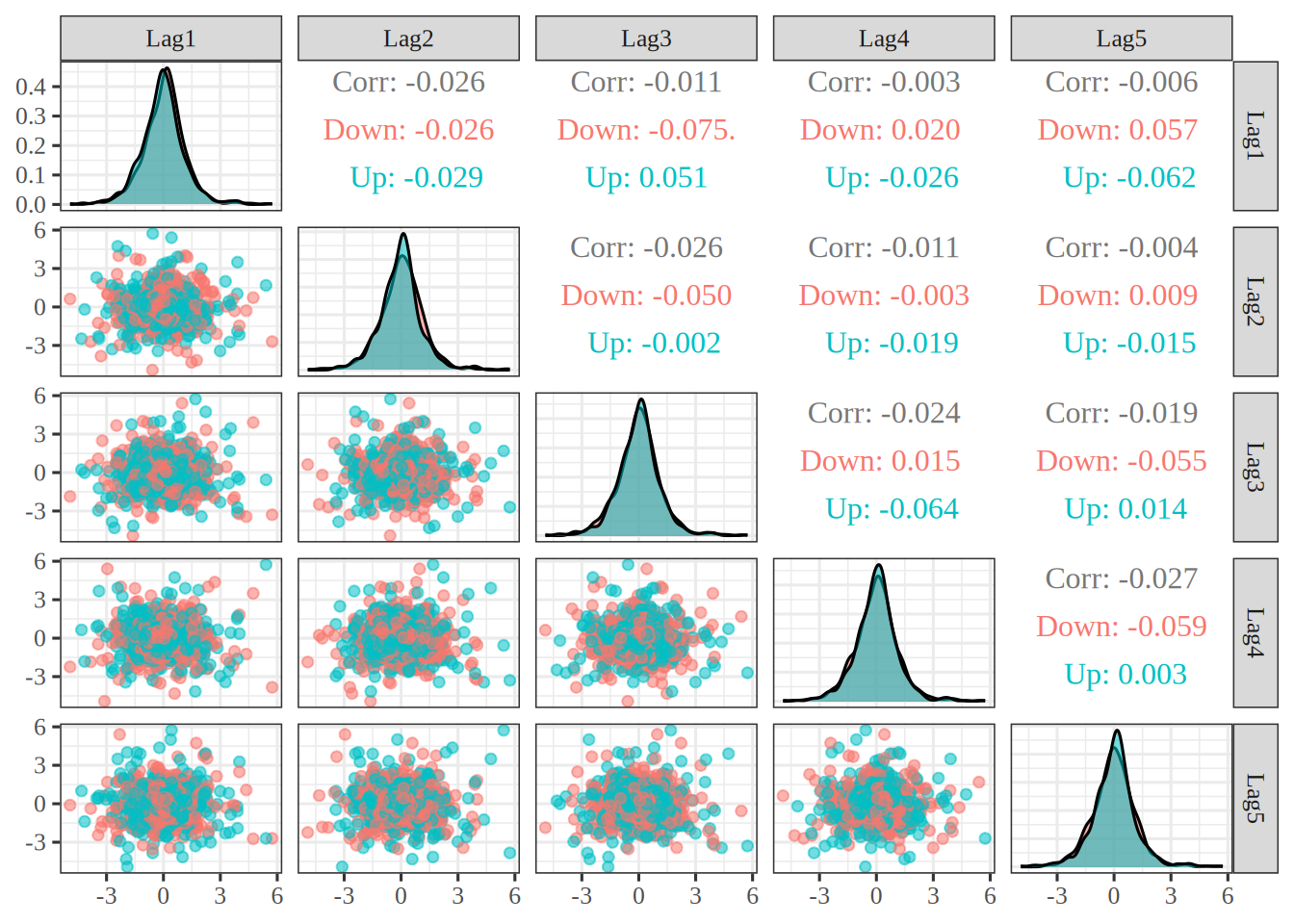
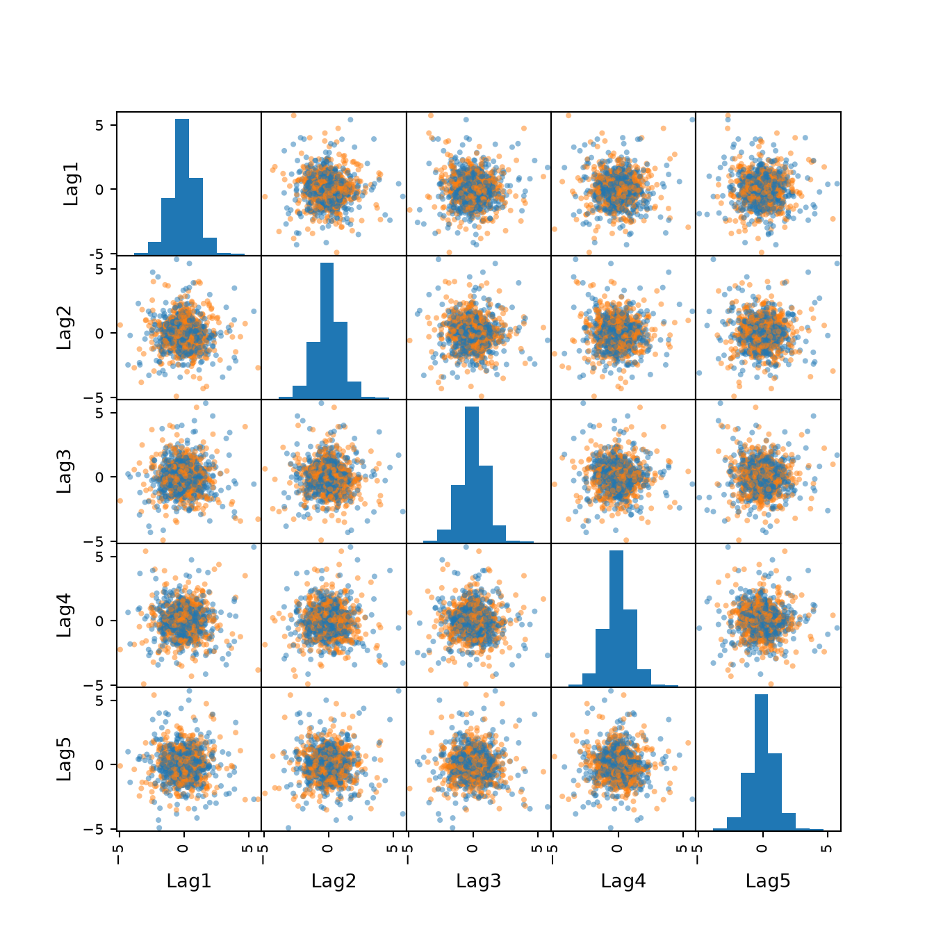
Exercise 3 (Lab: scatterplots of the lagged returns) Use the Smarket data. Draw a scatterplot of every two different columns from Lag1 to Lag5, with the points colored by Direction.

TipHint

In R, the ggpairs() function of the GGally package draws all the scatterplots of a data frame’s columns in one grid. In Python, the scatter_matrix() function of pandas.plotting does the same.

Solution 3. This solution continues Solution 2.

Figure 1: Plots of every two of the five lagged returns, with the up days and down days marked by color.
import matplotlib.pyplot as plt
from pandas.plotting import scatter_matrix

direction_colors = eda_py["Direction"].map({"Up": "tab:blue", "Down": "tab:orange"})
scatter_matrix(
    eda_py[lag_cols],
    c=direction_colors,
    alpha=0.5,
    figsize=(7, 7),
);
plt.show()

Grid of scatterplots of every two of the columns Lag1 to Lag5, with a histogram of each column on the diagonal. In every panel the points form one round cloud centred near zero, and the up days and down days overlap completely.

library(GGally) # nolint: undesirable_function_linter

lag_pairs <- eda_r |>
  ggpairs(columns = lag_cols, mapping = aes(color = Direction, alpha = 0.5))
lag_pairs

Grid of scatterplots of every two of the columns Lag1 to Lag5, with a density curve of each column on the diagonal and the correlation of each pair above it. In every panel the points form one round cloud centred near zero, and the up days and down days overlap completely.

In every panel of Figure 1, the dots form a round cloud centered near zero, which is the picture of the near-zero correlations from Solution 2. The up days and down days overlap completely, so no single lagged return, and no pair of them, separates the two classes by eye.

ExrExercise 4 (Lab: a histogram of the previous day’s return)

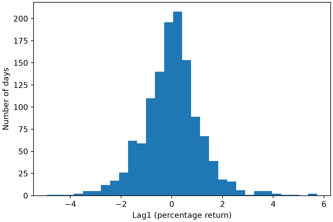
Exercise 4 (Lab: a histogram of the previous day’s return) Use the Smarket data. Draw a histogram of Lag1.

TipHint

The plotting functions draw a histogram of one column.

Solution 4. This solution continues Solution 1.

Figure 2: Bars counting the trading days at each value of the previous day’s percentage return, Lag1.
import matplotlib.pyplot as plt

fig, ax = plt.subplots(figsize=(6, 4), layout="constrained")
ax.hist(eda_py["Lag1"], bins=30);
ax.set_xlabel("Lag1 (percentage return)");
ax.set_ylabel("Number of days");
plt.show()

Histogram of the previous day's percentage return, Lag1, for every trading day in the data. The bars form one tall, narrow hump centred near zero, with thin tails and a few isolated bars far out on both sides.

library(ggplot2) # nolint: undesirable_function_linter

lag1_histogram <- eda_r |>
  ggplot() +
  aes(x = Lag1) +
  geom_histogram(bins = 30) +
  labs(x = "Lag1 (percentage return)", y = "Number of days")
is_html <- knitr::is_html_output()
if (is_html) {
  widget <- plotly::ggplotly(lag1_histogram) |>
    plotly::config(displaylogo = FALSE, responsive = TRUE)
  htmltools::div(role = "img", `aria-label` = lag1_histogram_alt, widget)
} else {
  lag1_histogram
}
Show code
eda_r_lag1_sd <- sd(eda_r$Lag1)
eda_r_within <- mean(abs(eda_r$Lag1) < 2 * eda_r_lag1_sd)
eda_r_per_bin <- nrow(eda_r) / 30

I chose 30 bins, which is about 42 days per bar on average. Far fewer bins would merge the thin tails into the central hump, and far more would leave most bars with only a few days, so the outline would look ragged. That trade-off is why 30 is a compromise between the two.

Figure 2 shows a single tall, narrow hump centered near zero, with thin tails on both sides. The sample mean is 0.004 and the standard deviation is 1.14, and 94.6% of the days lie within two of those spreads of the sample mean.

ExrExercise 5 (Lab: trading volume by year)

Exercise 5 (Lab: trading volume by year) Use the Smarket data. In which Year is the sample mean of Volume the largest?

TipHint

Split a column by the values of another before taking the sample mean, then find the group with the largest result.

Solution 5. This solution continues Solution 1.

eda_py_volume = eda_py.groupby("Year")["Volume"].mean()
eda_py_year = int(eda_py_volume.idxmax())
eda_py_volume.round(3)
Year
2001    1.227
2002    1.428
2003    1.385
2004    1.424
2005    1.917
Name: Volume, dtype: float64
eda_r_volume <- tapply(eda_r$Volume, eda_r$Year, mean)
eda_r_peak <- which.max(eda_r_volume)
eda_r_year <- names(eda_r_peak)
round(eda_r_volume, 3)
 2001  2002  2003  2004  2005 
1.227 1.428 1.385 1.424 1.917 

The sample mean of Volume is largest in 2005, at 1.917 billion shares. Volume rises over the period, although not every year, so a model that uses Volume can pick up the trend in time.

ExrExercise 6 (Lab: trading volume over time)

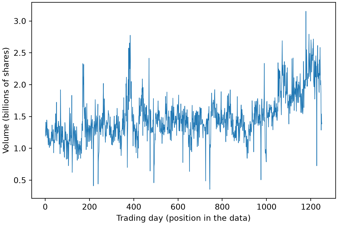
Exercise 6 (Lab: trading volume over time) Use the Smarket data. Plot Volume against the position of the trading day in the data, from the first day to the last.

TipHint

The plotting functions draw a scatterplot, and the row numbers are a sequence of whole numbers from the first row to the last.

Solution 6. This solution continues Solution 1.

Figure 3: The daily trading volume against the position of the day in the data.
import matplotlib.pyplot as plt

fig, ax = plt.subplots(figsize=(6, 4), layout="constrained")
ax.plot(eda_py.index + 1, eda_py["Volume"], linewidth=0.7);
ax.set_xlabel("Trading day (position in the data)");
ax.set_ylabel("Volume (billions of shares)");
plt.show()

Line plot of daily trading volume against the position of the day in the data, from the first day to the last. The line is jagged from day to day, roughly level for most of the period and higher over the last stretch, with a few sharp spikes and dips.

library(ggplot2) # nolint: undesirable_function_linter

eda_r_days <- dplyr::mutate(eda_r, day = dplyr::row_number())
volume_series <- eda_r_days |>
  ggplot() +
  aes(x = day, y = Volume) +
  geom_line(linewidth = 0.3) +
  labs(
    x = "Trading day (position in the data)",
    y = "Volume (billions of shares)"
  )
is_html <- knitr::is_html_output()
if (is_html) {
  widget <- plotly::ggplotly(volume_series) |>
    plotly::config(displaylogo = FALSE, responsive = TRUE)
  htmltools::div(role = "img", `aria-label` = volume_series_alt, widget)
} else {
  volume_series
}
Show code
eda_r_days_cor <- cor(eda_r_days$day, eda_r_days$Volume)

In Figure 3, volume is noisy from day to day, roughly level for most of the period and higher over the last stretch, which agrees with the yearly sample means in Solution 5. The correlation between the position of the day and Volume is 0.55.

ExrExercise 7 (Lab: the previous day’s return by direction)

Exercise 7 (Lab: the previous day’s return by direction) Use the Smarket data. Compute the sample mean of Lag1 within each value of Direction.

TipHint

Split a column by the values of another before taking the sample mean of each group.

Solution 7. This solution continues Solution 1.

eda_py_lag1 = eda_py.groupby("Direction")["Lag1"].mean()
eda_py_lag1.round(3)
Direction
Down    0.051
Up     -0.040
Name: Lag1, dtype: float64
eda_r_lag1 <- tapply(eda_r$Lag1, eda_r$Direction, mean)
round(eda_r_lag1, 3)
  Down     Up 
 0.051 -0.040 

The sample means are 0.051 on down days and -0.04 on up days. The difference is small next to the day-to-day spread of the returns, so Lag1 alone will not separate up days from down days well.

ExrExercise 8 (Lab: boxplots of the previous day’s return by direction)

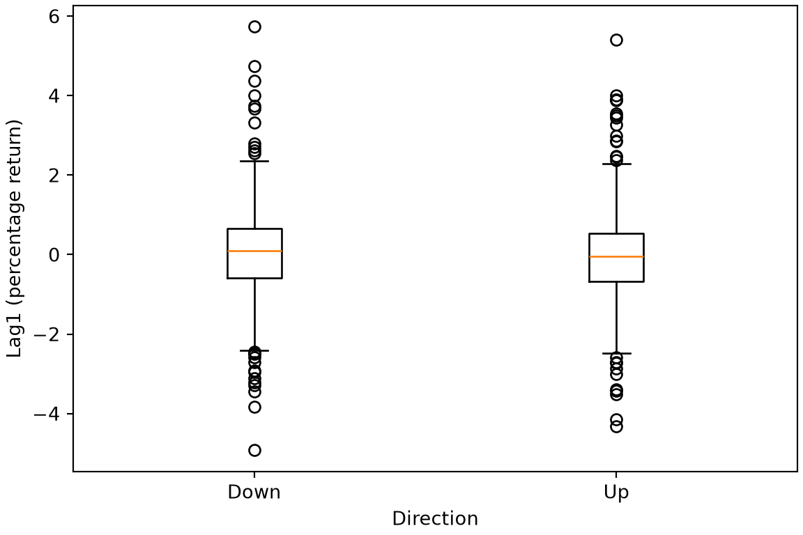
Exercise 8 (Lab: boxplots of the previous day’s return by direction) Use the Smarket data. Draw side-by-side boxplots of Lag1, one for each value of Direction.

TipHint

The boxplot methods take one array of values for each group, and you can select the rows of each group with a mask.

Solution 8. This solution continues Solution 1.

Figure 4: Boxplots of the previous day’s percentage return, Lag1, for the down days and the up days.
import matplotlib.pyplot as plt

by_direction = [
    eda_py.loc[eda_py["Direction"] == "Down", "Lag1"],
    eda_py.loc[eda_py["Direction"] == "Up", "Lag1"],
]
fig, ax = plt.subplots(figsize=(6, 4), layout="constrained")
ax.boxplot(by_direction, tick_labels=["Down", "Up"]);
ax.set_xlabel("Direction");
ax.set_ylabel("Lag1 (percentage return)");
plt.show()

Two side-by-side boxplots of the previous day's percentage return, Lag1, one for down days and one for up days. The two boxes sit at almost the same height, both centred near zero and with similar spreads, and many separate points beyond the whiskers in each.

library(ggplot2) # nolint: undesirable_function_linter

lag1_boxplot <- eda_r |>
  ggplot() +
  aes(x = Direction, y = Lag1) +
  geom_boxplot() +
  labs(x = "Direction", y = "Lag1 (percentage return)")
is_html <- knitr::is_html_output()
if (is_html) {
  widget <- plotly::ggplotly(lag1_boxplot) |>
    plotly::config(displaylogo = FALSE, responsive = TRUE)
  htmltools::div(role = "img", `aria-label` = lag1_boxplot_alt, widget)
} else {
  lag1_boxplot
}

In Figure 4, the two boxes overlap almost completely, which agrees with the small difference between the sample means in Solution 7. The boxplots add that the spreads are alike too, so Lag1 alone has little power to tell the two directions apart.

ExrExercise 9 (Lab: logistic regression on the stock market data)

Exercise 9 (Lab: logistic regression on the stock market data) Use the Smarket data. Fit a logistic regression for the probability that Direction is Up, using all the days. Take Lag1 to Lag5 and Volume as the predictors. Report each coefficient’s estimate, standard error, and \(p\)-value.

TipHint

The family argument chooses the logistic regression, and the summary of the fit holds each estimate, standard error, and \(p\)-value.

Solution 9.

import pandas as pd
import statsmodels.api as sm
import statsmodels.formula.api as smf

lab_py = pd.read_csv("data/smarket.csv")
lab_py["up"] = (lab_py["Direction"] == "Up").astype(int)
lab_py_fit = smf.glm(
    "up ~ Lag1 + Lag2 + Lag3 + Lag4 + Lag5 + Volume",
    data=lab_py,
    family=sm.families.Binomial(),
).fit()
lab_py_table = lab_py_fit.summary2().tables[1]
lab_py_table.round(3)
           Coef.  Std.Err.      z  P>|z|  [0.025  0.975]
Intercept -0.126     0.241 -0.523  0.601  -0.598   0.346
Lag1      -0.073     0.050 -1.457  0.145  -0.171   0.025
Lag2      -0.042     0.050 -0.845  0.398  -0.140   0.056
Lag3       0.011     0.050  0.222  0.824  -0.087   0.109
Lag4       0.009     0.050  0.187  0.851  -0.089   0.107
Lag5       0.010     0.050  0.208  0.835  -0.087   0.107
Volume     0.135     0.158  0.855  0.392  -0.175   0.446
lab_r <- readr::read_csv("data/smarket.csv", show_col_types = FALSE)
lab_r <- dplyr::mutate(lab_r, up = as.integer(Direction == "Up"))
lab_r_fit <- glm(
  up ~ Lag1 + Lag2 + Lag3 + Lag4 + Lag5 + Volume,
  data = lab_r,
  family = binomial
)
lab_r_table <- summary(lab_r_fit)$coefficients
round(lab_r_table, 3)
            Estimate Std. Error z value Pr(>|z|)
(Intercept)   -0.126      0.241  -0.523    0.601
Lag1          -0.073      0.050  -1.457    0.145
Lag2          -0.042      0.050  -0.845    0.398
Lag3           0.011      0.050   0.222    0.824
Lag4           0.009      0.050   0.187    0.851
Lag5           0.010      0.050   0.208    0.835
Volume         0.135      0.158   0.855    0.392
ExrExercise 10 (Lab: logistic regression on the stock market data (part 2))

Exercise 10 (Lab: logistic regression on the stock market data (part 2)) Use the fit of the logistic regression in Exercise 9. Which predictor has the smallest \(p\)-value?

TipHint

The summary of the fit holds one \(p\)-value for each coefficient.

Solution 10. This solution continues Solution 9.

Show code
lab_r_slopes <- lab_r_table[-1, , drop = FALSE]
lab_r_smallest <- rownames(lab_r_slopes)[which.min(lab_r_slopes[, 4])]
lab_r_smallest_p <- min(lab_r_slopes[, 4])
lab_r_verdict <- ifelse(lab_r_smallest_p < 0.05, "below", "above")

Lag1 has the smallest \(p\)-value, 0.15, which is above \(0.05\).

ExrExercise 11 (Lab: test the six predictors together)

Exercise 11 (Lab: test the six predictors together) Use the fit of Exercise 9. Take the drop from the null deviance to the deviance of that fit. What is the \(p\)-value of the drop, under the distribution of the drop?

TipHint

The fitted results hold the deviance of the fit and its null deviance, and the distribution of the drop is a chi-squared distribution, whose tail probability SciPy computes. In R, pchisq() plays that role.

Solution 11. This solution continues Solution 9.

from scipy import stats

lab_py_drop = lab_py_fit.null_deviance - lab_py_fit.deviance
lab_py_drop_df = lab_py_fit.df_model
lab_py_drop_p = float(stats.chi2.sf(lab_py_drop, lab_py_drop_df))
round(float(lab_py_drop), 2), round(lab_py_drop_p, 3)
(3.59, 0.732)
lab_r_drop <- lab_r_fit$null.deviance - lab_r_fit$deviance
lab_r_drop_df <- lab_r_fit$df.null - lab_r_fit$df.residual
lab_r_drop_p <- pchisq(lab_r_drop, df = lab_r_drop_df, lower.tail = FALSE)
lab_r_drop_both <- c(lab_r_drop, lab_r_drop_p)
round(lab_r_drop_both, 3)
[1] 3.591 0.732

The drop in deviance is 3.59, with a \(p\)-value of 0.732. The drop tests all 6 coefficients together, and it agrees with the coefficient table of Solution 9: no single predictor is clearly distinguishable from zero, and the six together do not improve clearly on a model with only an intercept.

ExrExercise 12 (Lab: a logistic regression with fewer predictors)

Exercise 12 (Lab: a logistic regression with fewer predictors) Use the split of Exercise 16. Fit a logistic regression for Direction on the days before \(2005\), with only Lag1 and Lag2 as predictors. Predict Up on a day in \(2005\) when the predicted probability is above \(0.5\). What is the accuracy on the test set?

TipHint

Fit the model with the family argument set to the binomial family, then compare the predicted probabilities on the test set with \(0.5\).

Solution 12.

lab_py_train = lab_py["Year"] < 2005
lab_py_small = smf.glm(
    "up ~ Lag1 + Lag2",
    data=lab_py[lab_py_train],
    family=sm.families.Binomial(),
).fit()
lab_py_prob = lab_py_small.predict(lab_py[~lab_py_train])
lab_py_up = (lab_py_prob > 0.5).astype(int)
lab_py_accuracy = float((lab_py_up == lab_py.loc[~lab_py_train, "up"]).mean())
lab_py_accuracy
0.5595238095238095
lab_r_train <- lab_r$Year < 2005
lab_r_small <- glm(
  up ~ Lag1 + Lag2,
  data = lab_r[lab_r_train, ],
  family = binomial
)
lab_r_prob <- predict(lab_r_small, lab_r[!lab_r_train, ], type = "response")
lab_r_up <- as.integer(lab_r_prob > 0.5)
lab_r_accuracy <- mean(lab_r_up == lab_r$up[!lab_r_train])
lab_r_accuracy
[1] 0.5595238

The accuracy is 56% in the R run and 56% in the Python run.

ExrExercise 13 (Lab: the confusion matrix on the test set)

Exercise 13 (Lab: the confusion matrix on the test set) Use the predictions of Exercise 12. Tabulate the predicted Direction against the actual Direction on the test set, as a confusion matrix.

TipHint

The counting functions tabulate each pair of values of two columns. The confusion matrix lists the predicted classes against the actual ones.

Solution 13. This solution continues Solution 12.

lab_py_actual = lab_py.loc[~lab_py_train, "Direction"]
lab_py_predicted = ["Up" if u == 1 else "Down" for u in lab_py_up]
pd.crosstab(
    pd.Series(lab_py_predicted, index=lab_py_actual.index, name="Predicted"),
    lab_py_actual.rename("Actual"),
)
Actual     Down   Up
Predicted           
Down         35   35
Up           76  106
lab_r_actual <- lab_r$Direction[!lab_r_train]
lab_r_predicted <- ifelse(lab_r_up == 1, "Up", "Down")
lab_r_confusion <- table(Predicted = lab_r_predicted, Actual = lab_r_actual)
lab_r_confusion
         Actual
Predicted Down  Up
     Down   35  35
     Up     76 106
Show code
lab_r_confusion_diag <- diag(lab_r_confusion)
lab_r_confusion_correct <- sum(lab_r_confusion_diag)
lab_r_confusion_total <- sum(lab_r_confusion)
lab_r_confusion_up <- sum(lab_r_predicted == "Up")

The confusion matrix covers 252 test days. The cells where the row and the column agree hold the 141 days classified correctly, so the accuracy is the same 56% as in Solution 12. The model predicts Up on 182 of those days.

ExrExercise 14 (Lab: the always-Up rule on the test set)

Exercise 14 (Lab: the always-Up rule on the test set) Use the split of Exercise 16. What is the accuracy on the test set of the rule that predicts Up on every day?

TipHint

A mask on a column of the test set counts the days on which Direction is Up. The accuracy is the share of days on which the prediction is right.

Solution 14. This solution continues Solution 12.

lab_py_baseline = float((lab_py.loc[~lab_py_train, "Direction"] == "Up").mean())
lab_py_baseline
0.5595238095238095
lab_r_test_direction <- lab_r$Direction[!lab_r_train]
lab_r_baseline <- mean(lab_r_test_direction == "Up")
lab_r_baseline
[1] 0.5595238

The rule is right exactly on the days that go up, so its accuracy is the share of Up days in the test set, 56%. The model of Solution 12 reaches 56%, which differs from this rule, one that uses no predictors, by 0 percentage points. On this data, the model’s accuracy is no better than that of always predicting Up.

ExrExercise 15 (Lab: predict at chosen values)

Exercise 15 (Lab: predict at chosen values) Use the fit of Exercise 12. What is the predicted probability that Direction is Up on a day with Lag1 \(= 1.2\) and Lag2 \(= 1.1\)?

TipHint

The predict function of the fit takes a data frame with the same columns as the predictors and returns predicted probabilities, not log-odds.

Solution 15.

lab_py_new = pd.DataFrame({"Lag1": [1.2], "Lag2": [1.1]})
lab_py_new_prob = float(lab_py_small.predict(lab_py_new).iloc[0])
round(lab_py_new_prob, 3)
0.479
lab_r_new <- tibble::tibble(Lag1 = 1.2, Lag2 = 1.1)
lab_r_new_prob <- predict(lab_r_small, lab_r_new, type = "response")
round(lab_r_new_prob, 3)
    1 
0.479 

The predicted probability is 0.48.

3 Training and test sets for the stock market data

ExrExercise 16 (Lab: split the Smarket data by year)

Exercise 16 (Lab: split the Smarket data by year) Split the Smarket data [1] into a training set of the days before \(2005\) and a test set of the days in \(2005\). Keep Lag1 and Lag2 as the predictors and Direction as the outcome.

TipHint

A mask on a column keeps the matching rows, and a selection of columns gives the predictors and the outcome.

Solution 16.

import pandas as pd

smarket = pd.read_csv("data/smarket.csv")
predictors = ["Lag1", "Lag2"]
is_train = smarket["Year"] < 2005
x_train = smarket.loc[is_train, predictors]
x_test = smarket.loc[~is_train, predictors]
y_train = smarket.loc[is_train, "Direction"]
y_test = smarket.loc[~is_train, "Direction"]
len(y_train), len(y_test)
(998, 252)
smarket <- readr::read_csv("data/smarket.csv", show_col_types = FALSE)
is_train <- smarket$Year < 2005
lag_cols <- c("Lag1", "Lag2")
x_train <- smarket[is_train, lag_cols]
x_test <- smarket[!is_train, lag_cols]
y_train <- smarket$Direction[is_train]
y_test <- smarket$Direction[!is_train]
n_train <- length(y_train)
n_test <- length(y_test)
c(n_train, n_test)
[1] 998 252

4 Poisson regression on bike rentals

RemarkRemark 1 (The bike rental exercises)

Remark 1 (The bike rental exercises). The book’s lab [1, Sec. 4.7.7] ends with a Poisson regression of the hourly Bikeshare counts, compared with a linear regression, which gives a negative count for some hours. Those exercises, and a first look at the data, are in the Poisson regression on bike rentals lab section.

References

[1]
G. James, D. Witten, T. Hastie, R. Tibshirani, and J. Taylor, An introduction to statistical learning: With applications in Python. Springer, 2023. doi: 10.1007/978-3-031-38747-0.
[2]
F. Pedregosa et al., “Scikit-learn: Machine learning in Python,” Journal of Machine Learning Research, vol. 12, pp. 2825–2830, 2011, Available: https://jmlr.org/papers/v12/pedregosa11a.html
[3]
A. Galanos, rugarch: Univariate GARCH models. 2026. doi: 10.32614/CRAN.package.rugarch.
Back to top