A First Model, End to End

Data, a model family, a loss, and learning as optimization

Published

Last modified: 2026-11-19

Show code
# reticulate provisions the Python packages that this page imports.
library(reticulate) # nolint: undesirable_function_linter
py_packages <- c("numpy", "pandas", "matplotlib", "SyncRNG")
py_require(py_packages)

Adapted from Brian Hutchinson’s Fall 2025 lecture notes, which supplied the crime-and-income example and its five neighborhoods. The figure the notes marked draw figure is Figure 1, and the two they marked plot are Figure 8 and Figure 10. Every fitted coefficient printed here is computed on the page from those same five points, and tools/make_big_ideas_figures.py fits the curves in the figures from them too. The wider reading is Hastie et al. [1], Chapter 2, and James et al. [2], Chapter 2.

The page Course Overview and the page Anatomy of a Learning Problem come first: they ask what machine learning is and define the vocabulary, where this page asks how one concrete instance of it works. Where they meet, this page recaps with a short exercise and links back to the definition.

1 The anatomy of a learning system

ExrExercise 1 (The parts of a learning system)

Exercise 1 (The parts of a learning system) Anatomy of a Learning Problem named the parts every learning system has. Without looking back, name them, and say which step happens once and which happens every time the system is used.

Solution 1. Figure 1 draws them. The training data go into a learning algorithm (the figure’s training algorithm), and running it, training, produces the model \(\modmem\). The model then maps each new input \(x\) to a prediction \(\modmemf{x}\).
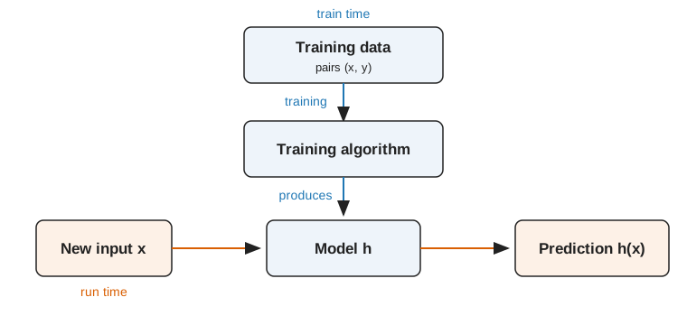
Figure 1: The two kinds of arrows in a learning system. The blue ones happen once, at train time; the orange ones happen every time the system is used, at run time.
Flow diagram. At train time, blue arrows lead from a box labeled training data, pairs (x, y), down into a box labeled training algorithm, which produces a box labeled model h. At run time, orange arrows lead from a box labeled new input x rightward into h, which outputs a box labeled prediction h(x).

Training, the blue arrows, happens once, at train time. Prediction, the orange arrows, happens every time the system is used, at run time. The difference matters for cost: a cost paid at train time is paid once, and a cost paid at run time is paid on every prediction forever.

2 A first model, end to end

We work with a data set, which the statistics notes define as \(n\) pairs of an input vector and its outcome. They also define its input matrix \(\mpredvar\), whose rows are the input vectors, and its outcome vector \(\voutvar\), whose entries are the outcomes. As that page notes, the “set” in training set, validation set and test set is short for a subset of the data set.

RemarkRemark 1 (The data set in matrix form)

Remark 1 (The data set in matrix form). Row \(i\) of \(\mpredvar\) and entry \(i\) of \(\voutvar\) together are the \(i\)-th pair of the data set, so \(\mpredvar\) and \(\voutvar\) hold the same information as \(\dataset\) in a tabular form.

ExmExample 1 (The Auto data as an input matrix)

Example 1 (The Auto data as an input matrix) Take the first five cars of the Auto data [2], with horsepower and weight as the \(\ninputvars = 2\) inputs and miles per gallon (mpg) as the outcome. Then \(\mpredvar\) has five rows and two columns, and \(\voutvar\) has five entries.

# Build the input matrix and outcome vector from the first five cars with a recorded horsepower.
import numpy as np
import pandas as pd

auto_five = pd.read_csv("data/auto.csv").dropna(subset=["horsepower"]).iloc[:5]
X_data = auto_five[["horsepower", "weight"]].to_numpy(dtype=float)
y_data = auto_five["mpg"].to_numpy(dtype=float)
print(X_data.shape, y_data.shape)
(5, 2) (5,)

Figure 2 draws the two arrays side by side. Row \(i\) of the left array and entry \(i\) of the right array are the same car.

Show code
import matplotlib.pyplot as plt

def show_array(ax, values, col_labels, title, fmt):
    """Draw a small array as a grid of cells, printing each value inside its cell."""
    # Shade each column on its own scale, because horsepower and weight differ by orders of magnitude.
    scaled = (values - values.min(axis=0)) / np.ptp(values, axis=0)
    ax.imshow(scaled, cmap="Blues", aspect="auto", vmin=0, vmax=1.6);
    for i in range(values.shape[0]):
        for j in range(values.shape[1]):
            ax.text(j, i, fmt.format(values[i, j]), ha="center", va="center", fontsize=9);
    ax.set_xticks(range(len(col_labels)), col_labels);
    ax.set_yticks(range(values.shape[0]), [f"{i + 1}" for i in range(values.shape[0])]);
    ax.set_title(title, fontsize=10);

fig, axes = plt.subplots(
    1, 2, figsize=(6, 2.8), layout="constrained",
    gridspec_kw={"width_ratios": [2, 1]},
)
show_array(axes[0], X_data, ["horsepower", "weight"], "input matrix X", "{:.0f}")
show_array(axes[1], y_data.reshape(-1, 1), ["mpg"], "outcome vector y", "{:.1f}")
plt.show()
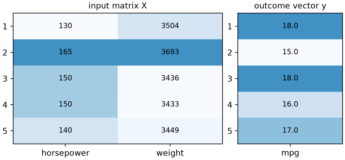
Figure 2: The input matrix of the first five Auto cars (left, one row per car, columns horsepower and weight) next to the outcome vector of their miles per gallon (right). Row i on the left and entry i on the right are the same car.
Two small tables of coloured cells drawn side by side. The left table has five rows and two columns labelled horsepower and weight. The right table is one column of five values labelled miles per gallon. Each row of the left table lines up with the entry in the same row of the right table.

The first car, for example, has input vector \(\vpredvar_1 = (130, 3504)\) and outcome \(\outvar_1 = 18\), and these fill the first row of the matrix and the first entry of the vector.

DefDefinition 1 (Parameter (weight, coefficient))

Definition 1 (Parameter (weight, coefficient)) A parameter of a prediction function family is a number that identifies one member of the family.

Other names: parameters are also called weights, and the parameters of a linear model are also called coefficients.

ExmExample 2 (The parameters of a line)

Example 2 (The parameters of a line) The straight line \(\modmemf{x} = mx + b\) has two parameters, the slope \(m\) and the intercept \(b\). Each pair of values for \(m\) and \(b\) picks out exactly one line.

RemarkRemark 2 (Training chooses the parameters)

Remark 2 (Training chooses the parameters). Training chooses the values of the parameters.

DatasetDataset 1: The crime and income data
Dataset 1: The crime and income data

Per-capita income and crime for 5 neighborhoods make up the crime data, taken from Brian Hutchinson’s Fall 2025 lecture notes [3]. The values were measured, not invented. Each variable was rescaled to run between 0 and 1. Their original source has been forgotten (Brian Hutchinson, personal communication, 2026). The data are in data/crime.csv, one neighborhood per line:

  • x: the neighborhood’s per-capita income, rescaled.
  • y: the outcome, the neighborhood’s crime rate, rescaled.
DefDefinition 2 (Training set)

Definition 2 (Training set) Given a data set \(\dataset\) of \(n\) pairs, a training set is the subset of \(\dataset\) whose pairs are indexed by a set \(\trainidx \subseteq \set{1, \ldots, n}\) to which we apply the fitting procedure, that is, the pairs from which the model’s parameters are estimated [4]:

\[ \trainset \eqdef \set{(\vpredvar_i, \outvar_i) : i \in \trainidx} \subseteq \dataset . \tag{1}\]
ExmExample 3 (Estimating a crime rate from income)

Example 3 (Estimating a crime rate from income) Suppose a city wants to estimate the crime rate in a neighborhood from that neighborhood’s per-capita income. An estimate would help it send police, outreach and services before the need appears in the data rather than after.

The city has the crime data (Dataset 1). The city’s data form a labeled data set of \(n\) pairs, written

\[ \dataset = \set{ \paren{\predvar_1, \outvar_1}, \ldots, \paren{\predvar_n, \outvar_n} } \]

and here \(n = 5\). Until we hold some pairs out, all of them form the training set, so \(\trainset = \dataset\):

Show code
# Read the five neighbourhoods once, from the local copy in data/crime.csv;
# every later example and figure on this page reuses this table.
crime <- read.csv("data/crime.csv")
knitr::kable(
  crime,
  col.names = c("per-capita income $x$", "crime rate $y$"),
  align = "rr", digits = 2
)
Table 1: The five sampled neighbourhoods. Both columns are rescaled to run between 0 and 1.
per-capita income \(x\) crime rate \(y\)
0.49 0.09
0.18 0.45
0.31 0.23
0.40 0.19
0.24 0.48
# The same table for the Python chunks.
import pandas as pd

crime = pd.read_csv("data/crime.csv")
print(crime.shape)
(5, 2)

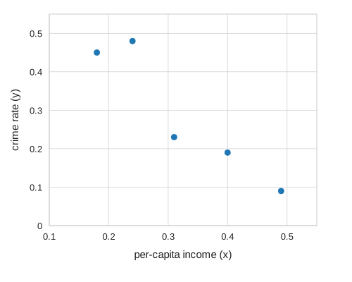
Where the numbers come from is in Dataset 1. Five neighborhoods are enough here, because the point being made is about the fitting procedure rather than about crime.

Figure 3: The five neighborhoods of Table 1.
A scatter plot of five points, crime rate against per-capita income. The points go from upper left to lower right: crime rate is generally lower at higher income.
ExrExercise 2 (What has the city already decided?)

Exercise 2 (What has the city already decided?) Before any model is fitted, the city’s setup has already made several choices that are not facts about the world. Name three, and say what each one rules out or risks.

Solution 2.

  • The goal is prediction, not description. We are not asking whether income causes crime, and nothing in this chapter justifies that interpretation. James et al. [2], Section 2.1.1, makes the same distinction between prediction and inference.

  • Income is the only input. It is almost certainly not the best one, and the model can only be as good as what it is shown.

  • The city sampled five neighborhoods. Five is a small number, and most of what goes wrong in this chapter goes wrong because of it.

ExrExercise 3 (What kind of task is this?)

Exercise 3 (What kind of task is this?) The outputs in Table 1 are crime rates. Say whether this is a regression task or a classification task, and say what about the table settles it.

Solution 3. Regression. The column of outputs holds numbers on a continuous scale, and the quantity we want back from the model is a number of the same kind. Had the city instead sorted neighborhoods into “high” and “low” crime, the same five neighborhoods would have posed a classification task.

The split is about the output, not about the inputs and not about the method. The inputs here are numbers too, and that is irrelevant; classification problems routinely have numeric inputs.

2.1 Choosing a model family

ExrExercise 4 (Propose a model)

Exercise 4 (Propose a model) Look at Figure 3. Propose a family of functions \(\modmem\) to predict \(y\) from \(x\), and say how many numbers have to be chosen to specify one member of your family.

Solution 4. The five points fall roughly along a line, so a reasonable family is the straight lines

\[ \modmemf{x} = mx + b \]

and two numbers identify exactly one: the slope \(m\) and the intercept \(b\).

Nothing yet says which \(m\) and \(b\) to pick; The next section, “Measuring how well a model fits”, starts on that.

Proposing a family by eye is honest here and does not work for larger problems. With one input we can look at the scatter plot; with fifty inputs there is no plot to look at, and the choice of family becomes a modeling decision argued from what the quantity is rather than from what the data looks like.

Training chooses from one mean-function model family, whose members are mean functions.

ExmExample 4 (The family of straight lines)

Example 4 (The family of straight lines) The straight lines

\[ \modmemf{x} = mx + b \tag{2}\]

form a mean-function model family, one line for each choice of the slope \(m\) and the intercept \(b\). Training on the five points picks one line from this family. No member of the family can bend, so a curved pattern in the data is out of its reach.

DefDefinition 3 (Fitted model)

Definition 3 (Fitted model) The fitted model \(\fitmodf{\trainset}\) is the model that a learning algorithm returns when it is applied to the training set \(\trainset\). It is a member of the mean-function model family, and it depends on \(\trainset\), so a different training set gives a different fitted model.

ExmExample 5 (A line fitted to the five neighborhoods)

Example 5 (A line fitted to the five neighborhoods) Let the learning algorithm fit a straight line by least squares, and let \(\trainset\) be the five neighborhoods of the crime data. The line that results is the fitted model \(\fitmodf{\trainset}\). Five other neighborhoods would give a different line, which is why the fitted model is random whenever the training set is.

DefDefinition 4 (Parametric model)

Definition 4 (Parametric model) A parametric model is a model family described by a fixed, finite list of parameters (Definition 1), whose length does not depend on the number of training points \(n\) [5].

ExmExample 6 (A line keeps two numbers however many cars it sees)

Example 6 (A line keeps two numbers however many cars it sees) In the Auto data [2], fit the straight line of mpg on horsepower (Equation 2) to the first 20, the first 100 and then all 392 cars. Count the parameters of the fitted model each time:

import numpy as np
import pandas as pd

auto_pm = pd.read_csv("data/auto.csv").dropna(subset=["horsepower"])
hp_pm = auto_pm["horsepower"].to_numpy(float)
mpg_pm = auto_pm["mpg"].to_numpy(float)

# np.polyfit returns the slope and the intercept: the line's whole description.
for n_pm in (20, 100, 392):
    coef_pm = np.polyfit(hp_pm[:n_pm], mpg_pm[:n_pm], 1)
    print(n_pm, len(coef_pm), coef_pm.round(3))
20 2 [-0.069 27.936]
100 2 [-0.101 31.46 ]
392 2 [-0.158 39.936]
auto_pm <- na.omit(read.csv("data/auto.csv")[, c("mpg", "horsepower")])

# Each column is one fit: its intercept, then its slope.
fits_pm <- sapply(c(20, 100, 392), function(n) {
  coef(lm(mpg ~ horsepower, data = auto_pm[1:n, ]))
})
colnames(fits_pm) <- c(20, 100, 392)
round(fits_pm, 3)
                20    100    392
(Intercept) 27.936 31.460 39.936
horsepower  -0.069 -0.101 -0.158

With 20 cars the slope is -0.069 miles per gallon per horsepower, and with all 392 it is -0.158. The values of the parameters change with the data, but the model keeps 2 of them whether it was fit to 20 cars or to 392. That fixed length makes the family of lines parametric (Definition 4).

Show code
library(ggplot2)
pmf_n <- c(20, 100, 392)
pmf_lines <- data.frame(
  cars = factor(pmf_n),
  intercept = fits_pm[1, ],
  slope = fits_pm[2, ]
)
ggplot(auto_pm, aes(horsepower, mpg)) +
  geom_point(colour = "grey60", alpha = 0.6) +
  geom_abline(
    data = pmf_lines,
    aes(intercept = intercept, slope = slope, colour = cars, linetype = cars)
  ) +
  scale_colour_manual(values = c("20" = "#0072B2", "100" = "#D55E00", "392" = "#009E73")) +
  scale_linetype_manual(values = c("20" = "solid", "100" = "dashed", "392" = "dotted")) +
  labs(x = "Horsepower", y = "Miles per gallon", colour = "Cars used", linetype = "Cars used")
Show code
import matplotlib.pyplot as plt
import numpy as np

fig, ax = plt.subplots(figsize=(6, 4), layout="constrained")
ax.plot(hp_pm, mpg_pm, color="grey", marker="o", linestyle="", alpha=0.6, markersize=4);
grid_pmf = np.array([hp_pm.min(), hp_pm.max()])
for n_pmf, colour, style in [(20, "#0072B2", "-"), (100, "#D55E00", "--"), (392, "#009E73", ":")]:
    slope_pmf, intercept_pmf = np.polyfit(hp_pm[:n_pmf], mpg_pm[:n_pmf], 1)
    ax.plot(grid_pmf, intercept_pmf + slope_pmf * grid_pmf, color=colour, linestyle=style,
            label=f"{n_pmf} cars");
ax.set_xlabel("Horsepower");
ax.set_ylabel("Miles per gallon");
fig.legend(loc="outside lower center", ncol=3);
plt.show()
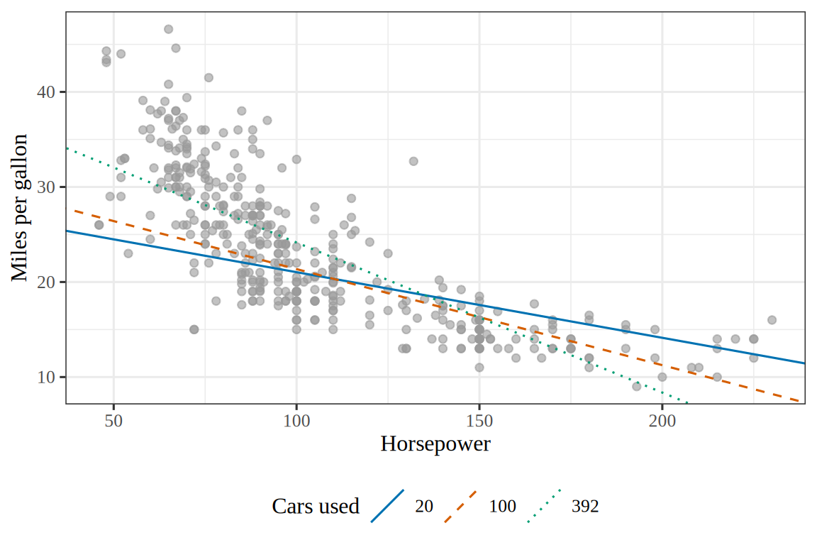
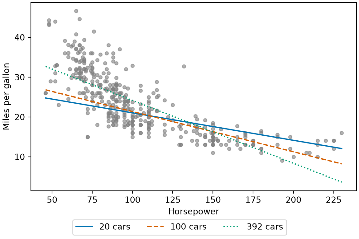
Figure 4: The three fitted models of Example 6, trained on the first 20, the first 100 and all of the cars. Each line is described by two numbers, however many cars it used.
(a)
Scatter plot of the miles per gallon of the 392 Auto cars against their horsepower, with the points falling along a curve that slopes down and flattens at high horsepower. Three straight lines are drawn through them, one fitted to the first 20 cars, one to the first 100 and one to all 392. The line for 20 cars is solid blue, the line for 100 cars is dashed vermilion and the line for 392 cars is dotted green. All three slope downward, and the line grows steeper as more cars are used, with the line for 392 cars the steepest.
(b)
Scatter plot of the miles per gallon of the 392 Auto cars against their horsepower, with the points falling along a curve that slopes down and flattens at high horsepower. Three straight lines are drawn through them, one fitted to the first 20 cars, one to the first 100 and one to all 392. The line for 20 cars is solid blue, the line for 100 cars is dashed vermilion and the line for 392 cars is dotted green. All three slope downward, and the line grows steeper as more cars are used, with the line for 392 cars the steepest.
ExmExample 7 (Straight lines are a parametric model)

Example 7 (Straight lines are a parametric model) The straight lines of Equation 2 form a parametric model with two parameters.

DefDefinition 5 (True mean function)

Definition 5 (True mean function) The true mean function \(\truemean\) is the mean function of the outcome \(\Outvar\) given the input \(\predvar\), taken over the whole population and not over a training set: \(\truemeanf{\predvar} = \condE{\Outvar}{\predvar}\).

ExmExample 8 (The true mean function of house prices)

Example 8 (The true mean function of house prices) Let the outcome \(\Outvar\) be the sale price of a house, and let the input \(\predvar\) be its floor area. The value of the true mean function at a floor area \(\predvar\) is the average sale price of all houses with that floor area. Two houses with the same floor area can sell for different prices, so the price of one house is not \(\truemeanf{\predvar}\) exactly.

DefDefinition 6 (Noise conditional on the input)

Definition 6 (Noise conditional on the input) The noise \(\noise\) of an observed outcome \(\Outvar\) conditional on the input \(\predvar\), as in the statistics notes, is the deviation of \(\Outvar\) from the value \(\truemeanf{\predvar}\) of the true mean function at \(\predvar\):

\[ \noise \eqdef \Outvar - \truemeanf{\predvar} . \]

ExmExample 9 (The noise of one car)

Example 9 (The noise of one car) When the 392 cars of the Auto data [2] form the population, with input \(\predvar\) equal to cylinders and outcome \(\Outvar\) equal to mpg, the true mean function value at \(\predvar = 4\) cylinders is \(\truemeanf{4} = 29.28\), the population mean of mpg for the 199 four-cylinder cars. The 1970 Datsun PL510 has \(\Outvar = 27.0\) mpg, so the noise for that car is \(\noise = 27.0 - 29.28 = -2.28\) mpg. The 1971 Toyota Corolla 1200 has \(\Outvar = 31.0\) mpg, so the noise for that car is \(\noise = 31.0 - 29.28 = 1.72\) mpg.

DefDefinition 7 (Noise model)

Definition 7 (Noise model) In the noise model, an input \(\predvar\) has outcome \(\Outvar\)

\[ \Outvar = \truemeanf{\predvar} + \noise, \qquad \E{\noise} = 0, \qquad \Var{\noise} = \varpar , \tag{3}\]

where \(\truemeanf{\predvar}\) is the value of the true mean function at \(\predvar\), \(\noise\) is the noise, conditional on \(\predvar\), with population mean \(\E{\noise} = 0\), and \(\varpar\) is the finite variance of \(\noise\) at \(\predvar\).

ExmExample 10 (The noise model for the four-cylinder cars)

Example 10 (The noise model for the four-cylinder cars) Take the cars of the Auto data [2] as in Example 9, with cylinders as \(\predvar\) and mpg as \(\Outvar\). The noise model writes the mpg of the 1970 Datsun PL510 as

\[ \begin{aligned} \Outvar &= \truemeanf{4} + \noise \\ &= 29.28 + (-2.28) \\ &= 27.0 . \end{aligned} \]

For the 199 four-cylinder cars, the noise model says that the noise has population mean \(0\), and that it has variance \(\varpar\) at \(\predvar = 4\).

VideosWatch

Hastie and Tibshirani introduce the regression function and how to estimate it, from 6:03 [6], video 2.1.

2.2 Measuring how well a model fits

ExrExercise 5 (What should a loss function do?)

Exercise 5 (What should a loss function do?) A loss function \(L(y, \hy)\) takes the true value \(y\) and a prediction \(\hy\) and returns one number saying how bad that prediction was. Before choosing a formula, decide what the formula has to satisfy.

Name two properties any such function needs, and for each one, name what goes wrong without it.

Solution 5. It is never negative. Without that, errors in opposite directions cancel in the average, and a model can get a lower loss for being wrong in the other direction. A signed error \(\hy - y\) does not satisfy this: a model that overshoots one point by 10 and undershoots the next by 10 averages to zero, which is the score a perfect model gets.

It is zero exactly when the prediction is right. Without that, “smaller is better” no longer has its usual meaning, and a perfect prediction can cost more than an imperfect one.

Two functions satisfy both:

\[ L_{2}(y, \hy) \eqdef (y - \hy)^2 \qquad\text{and}\qquad L_{1}(y, \hy) \eqdef \abs{ y - \hy } \tag{4}\]

We use squared error, \(L_2\), throughout this chapter. It has a third property the other lacks, and that property is about solving the problem rather than about stating it: squared error is differentiable everywhere, while absolute error has no derivative at the one point where the prediction is exact. The methods that search for a minimum step by step, starting with Gradient Descent, need that derivative.

The choice has consequences. Squaring an error of 10 costs a hundred times an error of 1, so \(L_2\) gives disproportionate weight to the worst-fitting points and a single outlier can pull the whole fit strongly toward it. \(L_1\) does not, which is exactly why robust regression uses it. Hastie et al. [1], Section 2.4, compares the two.

DefDefinition 8 (Loss function)

Definition 8 (Loss function) A loss function \(\lossf{y, \hy}\) takes the true value \(y\) and a prediction \(\hy\) and returns a number, never negative, saying how bad that prediction was [7].

RemarkRemark 3 (Which properties a loss needs, and what a loss scores)

Remark 3 (Which properties a loss needs, and what a loss scores). The two losses of Equation 4 also have the second property of Solution 5: they are zero exactly when \(\hy = y\). The definition of a loss function asks only for the first, because some losses later in these notes do not have the second: the hinge loss is zero for every score beyond the margin, and the loss for a predicted probability, which the chapter on fitting logistic regression defines, is never exactly zero.

A loss scores one prediction. For the \(i\)-th example, that prediction is the fitted value \(\hy_i = \modmemf{x_i}\), the value the model \(\modmem\) returns at \(x_i\), so the example’s loss is \(L(y_i, \hy_i)\). Other sources call an average of losses over many examples the cost or the objective.

Show code
# HTML formats get an interactive plotly figure (hover for values, click the
# legend to hide a curve); the handout and other formats get the same curves
# as a static SVG from tools/make_big_ideas_figures.py.
if (knitr::is_html_output()) {
  library(plotly)

  # Squared error and absolute error on a grid of errors.
  error <- seq(-2, 2, length.out = 401)

  widget <- plot_ly() |>
    add_trace(
      x = error, y = error^2, type = "scatter", mode = "lines",
      name = "squared error", line = list(color = "#1f77b4")
    ) |>
    add_trace(
      x = error, y = abs(error), type = "scatter", mode = "lines",
      name = "absolute error", line = list(color = "#d95f02", dash = "dash")
    ) |>
    layout(
      xaxis = list(title = "prediction minus truth"),
      yaxis = list(title = "loss", range = c(0, 4)),
      legend = list(orientation = "h", y = -0.2),
      margin = list(t = 10)
    ) |>
    config(displaylogo = FALSE, responsive = TRUE)

  # The alt text: a plotly widget has none of its own.
  htmltools::div(
    role = "img",
    `aria-label` = paste(
      "Interactive plot of squared error and absolute error against the error.",
      "Both are zero only at zero error; squared error is a smooth U and",
      "absolute error is a V with a corner at zero."
    ),
    widget
  )
} else {
  knitr::include_graphics("../images/big-ideas/losses.svg")
}
Figure 5: Squared error and absolute error as functions of the error, prediction minus truth. Both are zero only at zero error and never negative. Beyond an error of 1, squared error grows faster; within 1, it is smaller.
ExrExercise 6 (Who chooses the loss?)

Exercise 6 (Who chooses the loss?) A frost alarm predicts, each evening, whether tonight will freeze. A false alarm (predict frost, no frost comes) costs one unit, the price of lighting the heaters. A missed frost (predict no frost, frost comes) costs a different amount that depends on what is growing. Over 100 evenings, 10 of which had frost, two alarms scored as follows:

Table 2: The frosts caught and the false alarms of each alarm over 100 evenings.
Alarm Frosts caught False alarms
Cautious 10 of 10 20 of 90
Relaxed 6 of 10 5 of 90

A commercial orchard loses 50 units to a missed frost. A balcony gardener loses 2. Compute the total cost of each alarm for each owner.

Solution 6. Each alarm’s cost is its missed frosts times the miss cost plus its false alarms times one. The Cautious alarm misses none; the Relaxed alarm misses four.

import pandas as pd

# Counts from the table: [missed frosts, false alarms] for each alarm.
mistakes_wc = pd.DataFrame({"Cautious": [10 - 10, 20], "Relaxed": [10 - 6, 5]},
                           index=["missed", "false alarm"])
# The only thing that differs between owners is the cost of a missed frost;
# a false alarm costs 1 for both.
miss_cost_wc = {"Orchard": 50, "Balcony": 2}

costs_wc = pd.DataFrame({
    owner: mistakes_wc.loc["missed"] * miss + mistakes_wc.loc["false alarm"] * 1
    for owner, miss in miss_cost_wc.items()
})
print(costs_wc)
          Orchard  Balcony
Cautious       20       20
Relaxed       205       13
# Counts from the table: missed frosts and false alarms for each alarm.
missed_wc <- c(Cautious = 10 - 10, Relaxed = 10 - 6)
false_alarms_wc <- c(Cautious = 20, Relaxed = 5)
# The only thing that differs between owners is the cost of a missed frost;
# a false alarm costs 1 for both.
miss_cost_wc <- c(Orchard = 50, Balcony = 2)

costs_wc <- sapply(miss_cost_wc, function(miss) missed_wc * miss + false_alarms_wc * 1)
costs_wc
         Orchard Balcony
Cautious      20      20
Relaxed      205      13

The orchard prefers the Cautious alarm, at 20 units to the Relaxed alarm’s 205. The balcony gardener prefers the Relaxed alarm, at 13 units to the Cautious alarm’s 20.

ExrExercise 7 (Who chooses the loss? (part 2))

Exercise 7 (Who chooses the loss? (part 2)) Use the setup of Exercise 6.

The two owners rank the alarms differently. What does that say about who should pick the loss function for a model that makes this prediction?

Solution 7. The two alarms and their predictions are the same for both owners, so the ranking cannot be a fact about the alarms. It comes from the costs, which belong to whoever lives with the mistakes. That is why a loss function is something the user sets: the formula should say how much each kind of mistake matters in the application, and only the user knows that. Accuracy, which counts a missed frost and a false alarm alike, would pick the Relaxed alarm for both owners (91 correct nights against 80), which is the right answer for the balcony and a costly one for the orchard.

DefDefinition 9 (Plausible loss)

Definition 9 (Plausible loss) A loss function is plausible for a model of the data when it follows from an assumption about how the data arise: minimizing it gives the maximum likelihood fit under that assumption.

ExmExample 11 (Squared error is plausible under Gaussian noise)

Example 11 (Squared error is plausible under Gaussian noise) Suppose the noise \(\noise\) of the noise model is independent across observations, each with a Gaussian distribution with mean zero and variance \(\varpar\). The negative log-likelihood of the observations is then the sum of their squared errors divided by \(2 \varpar\), plus a constant that does not depend on the model. Minimizing the squared error therefore gives the maximum likelihood fit, so squared error is plausible under this assumption. For a binary outcome modeled as conditionally Bernoulli, the same reasoning with maximum likelihood yields a different loss, which the chapter on fitting logistic regression derives.

DefDefinition 10 (Friendly loss)

Definition 10 (Friendly loss) A loss function is friendly for a model family when the model that minimizes it can be found reliably and cheaply.

ExmExample 12 (Squared error and convex losses are friendly)

Example 12 (Squared error and convex losses are friendly) For a linear model, squared error has a closed-form solution, so no search is needed. More generally, every local minimum of a convex loss is a global one, so gradient descent cannot get stuck at a worse model. Both cases are friendly in the sense of Definition 10. Figure 6 contrasts a convex loss with one that is not convex.

Show code
fl_y <- c(1, 0, 0, 1, 1, 0)
fl_b <- seq(-2, 2, length.out = 201)
fl_steps_convex <- purrr::accumulate(
  1:8, \(b, i) b - 0.05 * sum(-2 * (fl_y - b)), .init = 2
)
fl_steps_bumpy <- purrr::accumulate(
  1:8, \(b, i) b - 0.05 * (4 * b^3 - 6 * b + 1), .init = 2
)
fl_at_convex <- c(fl_b, fl_steps_convex)
fl_at_bumpy <- c(fl_b, fl_steps_bumpy)
fl_loss_convex <- purrr::map_dbl(fl_at_convex, \(b) sum((fl_y - b)^2))
fl_loss_bumpy <- fl_at_bumpy^4 - 3 * fl_at_bumpy^2 + fl_at_bumpy
fl_models <- c("convex", "not convex")
fl_curve_b <- c(fl_b, fl_b)
fl_curve_convex <- fl_loss_convex[1:201]
fl_curve_bumpy <- fl_loss_bumpy[1:201]
fl_curve_loss <- c(fl_curve_convex, fl_curve_bumpy)
fl_curve_model <- rep(fl_models, each = 201)
fl_curve <- tibble::tibble(
  b = fl_curve_b, loss = fl_curve_loss, model = fl_curve_model
)
fl_path_b <- c(fl_steps_convex, fl_steps_bumpy)
fl_path_convex <- fl_loss_convex[202:210]
fl_path_bumpy <- fl_loss_bumpy[202:210]
fl_path_loss <- c(fl_path_convex, fl_path_bumpy)
fl_path_model <- rep(fl_models, each = 9)
fl_path <- tibble::tibble(
  b = fl_path_b, loss = fl_path_loss, model = fl_path_model
)
fl_curve |>
  ggplot2::ggplot() +
  ggplot2::aes(b, loss) +
  ggplot2::geom_line(colour = "#0072B2") +
  ggplot2::geom_point(data = fl_path, colour = "#D55E00") +
  ggplot2::facet_wrap(ggplot2::vars(model), scales = "free_y") +
  ggplot2::labs(x = "Parameter", y = "Loss")
Show code
import matplotlib.pyplot as plt
import numpy as np

fl_y = np.array([1, 0, 0, 1, 1, 0])
fl_models = {
    "convex": (lambda b: np.sum((fl_y - b) ** 2),
               lambda b: np.sum(-2 * (fl_y - b))),
    "not convex": (lambda b: b ** 4 - 3 * b ** 2 + b,
                   lambda b: 4 * b ** 3 - 6 * b + 1),
}
grid_fl = np.linspace(-2, 2, 201)
fig, axes = plt.subplots(1, 2, figsize=(7, 4), layout="constrained")
for ax, (name, (loss, grad)) in zip(axes, fl_models.items()):
    steps = [2.0]
    for _ in range(8):
        steps.append(steps[-1] - 0.05 * grad(steps[-1]))
    ax.plot(grid_fl, [loss(b) for b in grid_fl], color="#0072B2");
    ax.plot(steps, [loss(b) for b in steps], color="#D55E00", marker="o", linestyle="");
    ax.set_title(name);
    ax.set_xlabel("Parameter");
axes[0].set_ylabel("Loss");
plt.show()
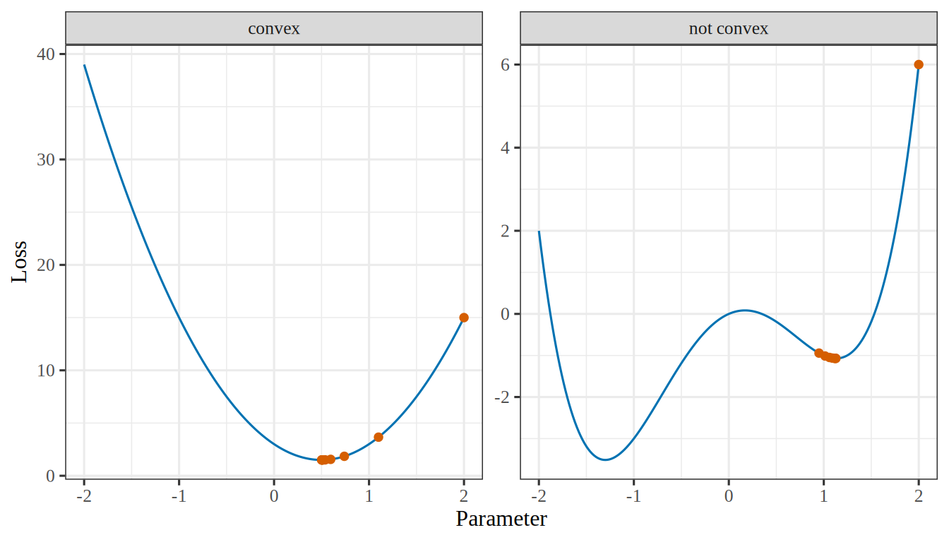
Figure 6: Gradient descent from \(2\) with step size \(0.05\) (points) on a convex loss and on a loss that is not convex. On the convex loss, here squared error, the descent approaches the one minimum. On the other, it stops at a local minimum that is not the lowest.
(a)
Two side-by-side line plots of a loss against a parameter, each with vermilion points marking gradient descent started at 2. Left, labelled convex: a blue U-shaped curve with one minimum at 0.5, and the points step down the right side and land on that minimum. Right, labelled not convex: a blue W-shaped curve with a deeper minimum near -1.3 and a shallower one near 1.1; the points step down the right side and stop at the shallower minimum, never reaching the deeper one.
(b)
Two side-by-side line plots of a loss against a parameter, each with vermilion points marking gradient descent started at 2. Left, labelled convex: a blue U-shaped curve with one minimum at 0.5, and the points step down the right side and land on that minimum. Right, labelled not convex: a blue W-shaped curve with a deeper minimum near -1.3 and a shallower one near 1.1; the points step down the right side and stop at the shallower minimum, never reaching the deeper one.
RemarkRemark 4 (When nobody specifies the loss)

Remark 4 (When nobody specifies the loss). Often the user cannot say what each mistake costs, or the costs are unknown when the model is fitted. Two other reasons then decide the loss: a plausible loss matches an assumption about the data, and a friendly loss is easy to optimize. Squared error is both, for the reasons in Example 11 and Example 12. A loss chosen for these reasons is a convenience, not a statement of what the errors cost, so it is worth checking the finished model against the costs that matter (Exercise 6).

This follows the discussion of error measures in Abu-Mostafa et al. [8, Ch. 1].

ExrExercise 8 (Score a model on data it has not seen)

Exercise 8 (Score a model on data it has not seen) The loss function scores a model on one pair at a time. A model is useful only if it also does well on points it has not seen. Suppose a new input–output pair \((X, Y)\) is drawn at random from the same population that produced the training data.

For a fixed model \(\modmem\), write the average loss that \(\modmem\) would incur over all such new pairs, as an expectation.

Solution 8. Average the loss over the distribution \(P(\predvar, \outvar)\) of inputs and outputs in the population:

\[ \Ep_{(\Predvar, \Outvar)} \sb{ \lossf{\Outvar, \modmemf{\Predvar}} } . \]

ExrExercise 9 (Score a model on data it has not seen (part 2))

Exercise 9 (Score a model on data it has not seen (part 2)) Use the setup of Exercise 8.

Which parts of your expression do you know, and which do you not know?

Solution 9. The loss function \(L\) is known, because we chose it, and the model \(\modmem\) is known, because we fitted it. The distribution \(P(\predvar, \outvar)\) is unknown, so the expectation cannot be computed. If we knew \(P(\predvar, \outvar)\), we would not need data to build a model.

DefDefinition 11 (Risk (expected loss, population risk, true risk, generalization error, expected prediction error))

Definition 11 (Risk (expected loss, population risk, true risk, generalization error, expected prediction error)) The risk of a model \(\modmem\) is its expected loss (Definition 8) on a new input–output pair \((X, Y)\) drawn from the joint distribution \(P(x, y)\) of the population:

\[ \popriskf{\modmem} \eqdef \Ep_{(X, Y)} \sb{ \lossf{Y, \modmemf{X}} } . \tag{5}\]

Other names: the risk is also called the expected loss, the population risk, the true risk, or the generalization error. The Elements of Statistical Learning calls it the expected prediction error [1, Sec. 2.4].

ExmExample 13 (Fitting a line to the crime data)

Example 13 (Fitting a line to the crime data) Fitting a line to the crime data, for example, is an attempt to pick the line \(\modmem\) whose squared error on neighborhoods we have not yet seen is small on average.

RemarkRemark 5 (The risk cannot be computed)

Remark 5 (The risk cannot be computed). The risk cannot be computed, because it needs the distribution the data came from, which we do not know. It can only be estimated from the data in hand.

The risk measures how well a model predicts neighborhoods outside the sample.

Every method in these notes tries to make \(\popriskf{\modmem}\) small.

The probability notes define risk for a prediction \(\hy\), which can be a constant or a function of \(X\). Here \(\hy = \modmemf{X}\).

DefDefinition 12 (Conditional risk (pointwise risk, risk at an input))

Definition 12 (Conditional risk (pointwise risk, risk at an input)) The conditional risk of a model \(\modmem\) at an input value \(\predvar\) is the expectation of its loss on a new output \(\Outvar\) drawn from the conditional distribution of \(\Outvar\) given \(\Predvar = \predvar\):

\[ \condpopriskf{\modmem}{\predvar} \eqdef \Expfc{\Outvar \mid \Predvar = \predvar}{ \lossf{\Outvar, \modmemf{\predvar}} } . \tag{6}\]

In words, it is the average loss of \(\modmem\) over the new pairs whose input is \(\predvar\).

ExmExample 14 (A line for the crime data, at one input value)

Example 14 (A line for the crime data, at one input value) Take a line \(\modmem\) chosen to predict the crime data, as in Example 13. Its conditional risk \(\condpopriskf{\modmem}{\predvar}\) is the expectation of the squared error on new neighborhoods whose input is exactly \(\predvar\). It can be small at an input where the line follows the data closely and large at an input where the line misses. The risk \(\popriskf{\modmem}\) is one number for the whole line, so it cannot show where the line fails.

RemarkRemark 6 (The risk is the average of the conditional risk)

Remark 6 (The risk is the average of the conditional risk). The risk is the average of the conditional risk over the distribution of the input \(\Predvar\):

\[ \popriskf{\modmem} = \Expfc{\Predvar}{ \condpopriskf{\modmem}{\Predvar} } . \tag{7}\]

This equality is the law of iterated expectations applied to \(\lossf{\Outvar, \modmemf{\Predvar}}\) in Equation 5: condition on \(\Predvar\), then average over \(\Predvar\).

The two quantities answer different questions. The conditional risk asks how well \(\modmem\) predicts at one input value. The risk asks how well \(\modmem\) predicts on average over all input values.

DefDefinition 13 (Empirical risk)

Definition 13 (Empirical risk) The empirical risk of a model \(\modmem\) on a data set \(\dataset\) is the average loss of \(\modmem\)’s predictions over the \(n\) pairs \((x_{(i)}, y_{(i)})\) of \(\dataset\):

\[ \empriskf{\modmem; \dataset} \eqdef \avgin \lossf{y_{(i)}, \modmemf{x_{(i)}}} . \tag{8}\]

RemarkRemark 7 (The empirical risk names its data set)

Remark 7 (The empirical risk names its data set). In the empirical risk, \(\dataset\) can be any data set: the training set the fitted model was fitted to, or data that played no part in the fit. The same model has a different empirical risk on each, so the notation always names the set.

DefDefinition 14 (Training error)

Definition 14 (Training error) The training error [1, Sec. 7.2] of a model \(\modmem\) is its empirical risk on the training set, \(\empriskf{\modmem; \trainset}\).

See training error in the statistics notes.

ExmExample 15 (Two models, scored on the same five neighborhoods)

Example 15 (Two models, scored on the same five neighborhoods) Score two models on the five neighborhoods of Table 1 under squared error: the least-squares line, and the constant that always predicts the sample mean crime rate.

# The five neighbourhoods of @tbl-crime-data, read once in @exm-crime-task.
x <- crime$x
y <- crime$y

emprisk_line <- mean(residuals(lm(y ~ x))^2)
emprisk_const <- mean((mean(y) - y)^2)
print(round(c(emprisk_line, emprisk_const), 6))
[1] 0.002721 0.023056
import numpy as np

# The five neighbourhoods of the crime table, read once in the first example.
x = crime["x"].to_numpy()
y = crime["y"].to_numpy()

m, b = np.polyfit(x, y, 1)
emprisk_line = np.mean((m * x + b - y) ** 2)
emprisk_const = np.mean((y.mean() - y) ** 2)
print(round(emprisk_line, 6), round(emprisk_const, 6))
0.002721 0.023056

The line’s empirical risk is \(0.002721\) and the constant’s is \(0.023056\). The line scores better on these five neighborhoods. Both models were fitted to them, so these are training errors, and the line fits the training set better. It says nothing yet about neighborhoods outside the sample, which the risk (Definition 11) measures.

Show code
library(ggplot2)
erf_fit <- lm(y ~ x, data = crime)
erf_levels <- c("least-squares line", "sample mean")
erf_models <- data.frame(
  model = factor(erf_levels, levels = erf_levels),
  intercept = c(coef(erf_fit)[[1]], mean(crime$y)),
  slope = c(coef(erf_fit)[[2]], 0)
)
erf_points <- merge(crime, erf_models)
erf_points$predicted <- erf_points$intercept + erf_points$slope * erf_points$x
ggplot(erf_points, aes(x, y)) +
  geom_abline(
    data = erf_models,
    aes(intercept = intercept, slope = slope, colour = model, linetype = model)
  ) +
  geom_segment(aes(xend = x, yend = predicted, colour = model, linetype = model)) +
  geom_point(size = 2.5) +
  facet_wrap(vars(model)) +
  scale_colour_manual(values = c("least-squares line" = "#0072B2", "sample mean" = "#D55E00")) +
  scale_linetype_manual(values = c("least-squares line" = "solid", "sample mean" = "dashed")) +
  guides(colour = "none", linetype = "none") +
  labs(x = "Explanatory variable", y = "Crime rate")
Show code
import matplotlib.pyplot as plt
import numpy as np

x_erf = crime["x"].to_numpy()
y_erf = crime["y"].to_numpy()
m_erf, b_erf = np.polyfit(x_erf, y_erf, 1)
grid_erf = np.array([x_erf.min(), x_erf.max()])
fig, axes = plt.subplots(1, 2, figsize=(7, 4), sharey=True, layout="constrained")
for ax, title, colour, style, intercept, slope in [
    (axes[0], "least-squares line", "#0072B2", "-", b_erf, m_erf),
    (axes[1], "sample mean", "#D55E00", "--", y_erf.mean(), 0),
]:
    predicted = intercept + slope * x_erf
    ax.plot(grid_erf, intercept + slope * grid_erf, color=colour, linestyle=style);
    ax.vlines(x_erf, predicted, y_erf, color=colour, linestyle=style);
    ax.plot(x_erf, y_erf, color="black", marker="o", linestyle="");
    ax.set_title(title);
    ax.set_xlabel("Explanatory variable");
axes[0].set_ylabel("Crime rate");
plt.show()
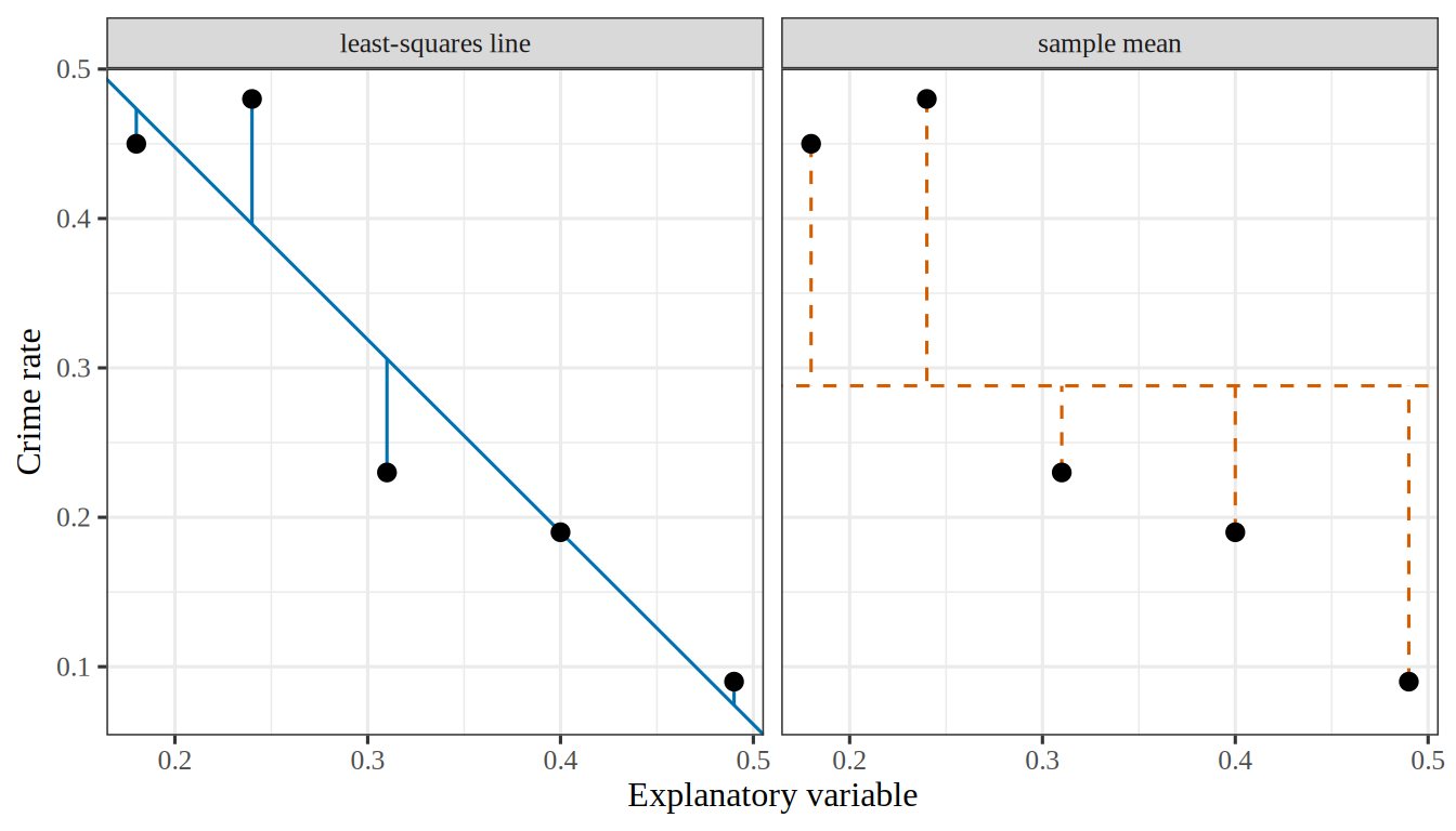
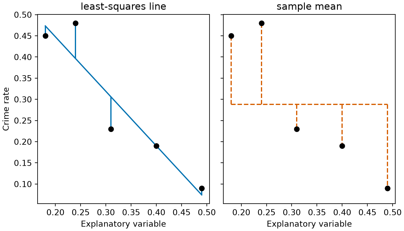
Figure 7: The two models of Example 15 on the five neighborhoods, each with the vertical distance from every point to it. The empirical risk is the average squared vertical distance from the points to either curve, which is smaller for the straight line than for the horizontal one.
(a)
Two side-by-side scatter plots of the crime rate against the explanatory variable for the same five neighbourhoods. The left panel, titled least-squares line, shows a solid blue straight line sloping steeply downward, with a short solid blue vertical segment from each point to the line, the longest about 0.08 long. The right panel, titled sample mean, shows a dashed vermilion horizontal line at the mean crime rate, with a dashed vermilion vertical segment from each point to the line. These segments are longer than those of the left panel, the longest about 0.2.
(b)
Two side-by-side scatter plots of the crime rate against the explanatory variable for the same five neighbourhoods. The left panel, titled least-squares line, shows a solid blue straight line sloping steeply downward, with a short solid blue vertical segment from each point to the line, the longest about 0.08 long. The right panel, titled sample mean, shows a dashed vermilion horizontal line at the mean crime rate, with a dashed vermilion vertical segment from each point to the line. These segments are longer than those of the left panel, the longest about 0.2.
RemarkRemark 8 (Empirical risk estimates the risk)

Remark 8 (Empirical risk estimates the risk). The empirical risk has a hat because it estimates the risk \(\popriskf{\modmem}\) of Equation 5 from the sample at hand: the sample average replaces the expectation. That average is over the empirical distribution of the pairs in the data set, which is what “empirical” refers to. On the training set the estimate tends to be too optimistic, because the model was fitted to those very pairs; the Generalization page estimates the risk from pairs that the fit did not use. Exercise 10, below, works the case of squared error and five points.

Unlike the risk, the empirical risk can be computed, because it needs only the data in hand and not the distribution they came from.

LemTheorem 1 (Under squared-error loss, the empirical risk is the sample mean squared error (sMSE))

Theorem 1 (Under squared-error loss, the empirical risk is the sample mean squared error (sMSE)) Let \(\lossf{\outvar, \eoutvar} = \sqf{\err}\) be the squared-error loss of Equation 4, where \(\err = \eoutvar - \outvar\) is the prediction error. For every model \(\modmem\) and every training set \(\trainset\) of \(n\) pairs, the empirical risk of \(\modmem\) on \(\trainset\) equals the sample mean squared error (sMSE) of \(\modmem\)’s predictions on \(\trainset\):

\[ \empriskf{\modmem; \trainset} = \sMSE{\modmem; \trainset} . \tag{9}\]

Proof. The empirical risk of Equation 8 is the average loss over the pairs of \(\trainset\). For example \(i\), the prediction error is \(\err_{(i)} = \modmemf{\predvar_{(i)}} - \outvar_{(i)}\). Substituting the squared-error loss into that average gives

\[ \empriskf{\modmem; \trainset} = \avgin \sqf{\err_{(i)}} . \]

The sMSE is the average of the squared differences between each label and its prediction, which are the squared prediction errors. The right-hand side above is exactly that average.

ExmExample 16 (The empirical risk and the sMSE of the least-squares line agree)

Example 16 (The empirical risk and the sMSE of the least-squares line agree) Compute the empirical risk of the least-squares line of Example 15 two ways: by averaging the squared-error loss example by example, and by applying the sMSE formula to the vector of residuals.

import numpy as np

# The five neighbourhoods of the crime table, read once in the first example.
x = crime["x"].to_numpy()
y = crime["y"].to_numpy()
m, b = np.polyfit(x, y, 1)

# Empirical risk: average the loss of each example separately.
def squared_error(y_true, y_pred):
    return (y_true - y_pred) ** 2

emprisk_by_loss = np.mean([squared_error(y_i, m * x_i + b) for x_i, y_i in zip(x, y)])

# MSE: square the residual vector, then average.
residuals = y - (m * x + b)
mse_by_residuals = np.sum(residuals ** 2) / len(y)

print(round(emprisk_by_loss, 6), round(mse_by_residuals, 6))
0.002721 0.002721

The two computations give \(0.002721\) and \(0.002721\), as Theorem 1 says they must. They differ only in how the arithmetic is organized.

DefDefinition 15 (Empirical risk minimization)

Definition 15 (Empirical risk minimization) Empirical risk minimization is choosing the \(\modmem\) that makes the empirical risk smallest [9].

ExrExercise 10 (Score a whole model, not one prediction)

Exercise 10 (Score a whole model, not one prediction) Equation 4 scores one prediction. Write an expression that scores a candidate \(\modmem\) against the whole training set \(\trainset\) of Table 1, using squared error.

Solution 10. Average the loss over the training points. That average is the empirical risk (Definition 13):

\[ \empriskf{\modmem; \trainset} \eqdef \avgin \lossf{y_{(i)}, \modmemf{x_{(i)}}} = \frac{1}{5} \sumto{i}{5} \paren{\modmemf{x_{(i)}} - y_{(i)}}^2 \tag{10}\]

ExrExercise 11 (Score a whole model, not one prediction (part 2))

Exercise 11 (Score a whole model, not one prediction (part 2)) Use the setup of Exercise 10.

Say which symbols in your expression are fixed and which are free to vary.

Solution 11. The \(x_{(i)}\) and \(y_{(i)}\) are fixed: they are the data, and they do not change. What can vary is \(\modmem\) — and since Equation 2 says \(\modmem\) is fixed by \(m\) and \(b\), Equation 10 is a function of those two numbers alone. Writing it that way turns the modeling question into an optimization problem:

\[ \hat{m}, \hat{b} \eqdef \argmin_{m, b} \empriskf{\modmem; \trainset} \tag{11}\]

These notes call solving Equation 11 training the model, also called learning.

ExrExercise 12 (Score a whole model, not one prediction (part 3))

Exercise 12 (Score a whole model, not one prediction (part 3)) Use the setup of Exercise 10.

Compare your expression with the risk of Equation 5. What does it use in place of the expectation?

Solution 12. Compared with the risk of Equation 5, the empirical risk replaces the expectation over \(P(x, y)\) with an average over the \(n\) points of \(\trainset\). Those points are the only draws from \(P(x, y)\) that we have.

The hat on \(\emprisk\) marks it as an estimate of the risk. The Generalization page says how badly it can mislead.

VideosWatch

Hutchinson works one example in which a model, a loss and the empirical risk appear, Machine Learning Example (21 min) [10]. The video site requires a login, which enrolled students find in the syllabus.

ReadingRead

2.3 Metrics

DefDefinition 16 (Metric)

Definition 16 (Metric) A metric of one or more models is a number computed from the models’ outputs and the true outputs on a data set.

ExmExample 17 (The sample mean squared error is a metric)

Example 17 (The sample mean squared error is a metric) The sample mean squared error (sMSE) of a model on a data set is a metric: it is computed from the model’s predictions and the true outputs. With the loss \(\lossf{\outvar, \eoutvar} = \sqf{\err}\) of Equation 4, the training error of a model is its sMSE on the training set, by Theorem 1.

DefDefinition 17 (Absolute metric)

Definition 17 (Absolute metric) An absolute metric is a metric that reports how accurate one model is, so its value for that model alone, compared with what the purpose requires, says whether the model is good enough.

ExmExample 18 (Absolute metric)

Example 18 (Absolute metric) On a test set, how often a classifier’s prediction is right is an absolute metric: it says how accurate the classifier is, whatever any other model does.

DefDefinition 18 (Relative metric)

Definition 18 (Relative metric) A relative metric is a metric of two models that says which of the two is better, without saying how accurate either one is.

ExmExample 19 (Relative metric)

Example 19 (Relative metric) On a test set, take the number of test examples on which model A has a smaller magnitude of prediction error than model B, minus the number on which B has the smaller one. That difference is a relative metric: a value above zero says that A is better than B, but it does not say whether either model is accurate enough to use.

DefDefinition 19 (Accuracy)

Definition 19 (Accuracy) The accuracy of a classifier on \(N\) examples is the fraction that it classifies correctly [13]. If \(M_{ij}\) is the number of examples in class \(i\) that it predicts as class \(j\), with \(C\) classes,

\[ \begin{aligned} \mathrm{Acc} &= \frac{\trf{M}}{N} \\ &= \frac{\sumto{c}{C} M_{cc}}{N}. \end{aligned} \]

DefDefinition 20 (Error rate)

Definition 20 (Error rate) The error rate of a classifier is the fraction of examples that it classifies incorrectly,

\[ \mathrm{Err} = 1 - \mathrm{Acc}, \]

where \(\mathrm{Acc}\) is its accuracy (Definition 19).

ExmExample 20 (Accuracy and error rate of a two-class classifier)

Example 20 (Accuracy and error rate of a two-class classifier) Suppose a classifier sorts \(N = 100\) emails into spam (class 1) or not spam (class 2), and \(M_{ij}\) counts the emails in class \(i\) that it predicts as class \(j\):

\[ M = \begin{bmatrix} 35 & 10 \\ 5 & 50 \end{bmatrix}. \]

It classifies the \(M_{11} + M_{22}\) emails on the diagonal correctly, so its accuracy is

\[ \begin{aligned} \mathrm{Acc} &= \frac{M_{11} + M_{22}}{N} \\ &= \frac{35 + 50}{100} \\ &= 0.85, \end{aligned} \]

and its error rate is

\[ \begin{aligned} \mathrm{Err} &= 1 - \mathrm{Acc} \\ &= 1 - 0.85 \\ &= 0.15. \end{aligned} \]

RemarkRemark 9 (Metric versus loss)

Remark 9 (Metric versus loss). A metric is usually not the loss that training minimizes. Training by gradient descent needs a loss that is differentiable. A person reads the metric, so it must be interpretable for the purpose at hand.

VideosWatch

2.4 Learning is optimization

ExrExercise 13 (Fit the line)

Exercise 13 (Fit the line) Solve Equation 11 for the five points of Table 1.

You do not need to do it by hand: every language these notes use has a least-squares routine. Report \(\hat{m}\), \(\hat{b}\), and the empirical risk the fitted line achieves.

TipHint

In Python, numpy.polyfit(x, y, 1). In R, lm(y ~ x).

Solution 13.

# The five neighbourhoods of @tbl-crime-data, read once in @exm-crime-task.
x <- crime$x
y <- crime$y

fit <- lm(y ~ x)
risk <- mean(residuals(fit)^2)
print(round(c(coef(fit)[["x"]], coef(fit)[["(Intercept)"]], risk), 6))
[1] -1.287671  0.705205  0.002721
import numpy as np

# The five neighbourhoods of the crime table, read once in the first example.
x = crime["x"].to_numpy()
y = crime["y"].to_numpy()

m, b = np.polyfit(x, y, 1)
risk = np.mean((m * x + b - y) ** 2)
print(round(m, 6), round(b, 6), round(risk, 6))
-1.287671 0.705205 0.002721

Both return the same fit,

\[ \emodmemf{x} = -1.2877\,x + 0.7052 \tag{12}\]

at an empirical risk of \(0.002721\). Figure 10 draws it.

Show code
# The empirical risk of the line m x + b on a grid of slopes and intercepts,
# for the five neighbourhoods the chapter fits. Both drawings below read it.
# The five neighbourhoods of @tbl-crime-data, read once in @exm-crime-task.
x <- crime$x
y <- crime$y

m_grid <- seq(-2.4, -0.2, by = 0.04)
b_grid <- seq(0.35, 1.05, by = 0.02)
risk_of <- function(m, b) mean((m * x + b - y)^2)
risk <- outer(m_grid, b_grid, Vectorize(risk_of))

# The least-squares line, the lowest point of the surface.
fit <- lm(y ~ x)
best_m <- coef(fit)[["x"]]
best_b <- coef(fit)[["(Intercept)"]]
best_risk <- risk_of(best_m, best_b)

# The levels of the contour lines, the same on the surface and in the plot.
levels <- c(0.004, 0.012, 0.030, 0.060, 0.100)
Show code
# The 3D surface of the empirical risk. HTML formats get an interactive plotly
# widget; the handout and other formats get the same surface from persp().
# The handout hides this code (echo above): a figure with its listing inside is
# taller than a page, and LaTeX then drops the float. The website folds it.

# Contour lines at the levels of the 2D plot below, drawn on the surface.
# contourLines() traces each level; NA rows separate the separate curves.
curves <- contourLines(m_grid, b_grid, risk, levels = levels)
lines <- do.call(rbind, lapply(curves, function(curve) {
  n <- length(curve$x)
  data.frame(
    m = c(curve$x, NA), b = c(curve$y, NA), risk = c(rep(curve$level, n), NA)
  )
}))

if (knitr::is_html_output()) {
  library(plotly)

  # What a hover shows, for the surface and for the minimum.
  hover <- paste0(
    "slope m: %{x:.3f}<br>intercept b: %{y:.3f}",
    "<br>empirical risk: %{z:.4f}<extra></extra>"
  )

  widget <- plot_ly() |>
    add_surface(
      x = m_grid, y = b_grid, z = t(risk), colorscale = "YlGnBu",
      colorbar = list(title = "empirical risk", len = 0.7),
      hovertemplate = hover
    ) |>
    add_trace(
      data = lines, x = ~m, y = ~b, z = ~risk,
      type = "scatter3d", mode = "lines",
      line = list(color = "#222222", width = 3), hoverinfo = "skip"
    ) |>
    add_trace(
      x = best_m, y = best_b, z = best_risk,
      type = "scatter3d", mode = "markers",
      marker = list(
        size = 6, color = "#d95f02", line = list(color = "#ffffff", width = 1)
      ),
      hovertemplate = sub("<extra></extra>", "<extra>minimum</extra>", hover)
    ) |>
    layout(
      showlegend = FALSE,
      margin = list(l = 0, r = 0, t = 0, b = 0),
      paper_bgcolor = "rgba(0,0,0,0)",
      scene = list(
        xaxis = list(title = "slope m"), yaxis = list(title = "intercept b"),
        zaxis = list(title = "empirical risk"),
        camera = list(eye = list(x = 1.5, y = -1.7, z = 0.9))
      )
    ) |>
    config(displaylogo = FALSE, responsive = TRUE)

  # The alt text: a plotly widget has none of its own.
  htmltools::div(
    role = "img",
    `aria-label` = paste(
      "Interactive 3D surface of the empirical risk over the slope and the",
      "intercept, a bowl with contour lines and one lowest point marked in",
      "orange. Drag to rotate and scroll to zoom."
    ),
    widget
  )
} else {
  # persp() returns the matrix that maps a point of the surface to the page,
  # which trans3d() applies to the contour lines and the minimum.
  z_hi <- 0.55
  shade <- colorRampPalette(c("#ffffcc", "#41b6c4", "#253494"))(50)
  # Colour each facet by the mean risk at its four corners.
  nr <- length(m_grid)
  nc <- length(b_grid)
  corner_mean <- (risk[-nr, -nc] + risk[-1, -nc] + risk[-nr, -1] + risk[-1, -1]) / 4
  facet_col <- shade[cut(corner_mean, 50, labels = FALSE)]
  par(mar = c(0, 0, 0, 0))
  view <- persp(
    m_grid, b_grid, pmin(risk, z_hi), zlim = c(0, z_hi), col = facet_col,
    border = NA, theta = 55, phi = 32, expand = 0.7, ticktype = "detailed", nticks = 4, cex.axis = 0.7,
    xlab = "slope m", ylab = "intercept b", zlab = "empirical risk"
  )
  segments_xy <- trans3d(lines$m, lines$b, pmin(lines$risk, z_hi), view)
  lines(segments_xy, col = "#222222", lwd = 1.5)
  points(trans3d(best_m, best_b, best_risk, view), pch = 21, bg = "#d95f02", col = "white", cex = 1.8)
}
Show code
# The same contours in 2D: each blue curve joins the lines with one
# empirical risk, and they close in on the least-squares line (orange).
par(mar = c(4.2, 4.2, 2.2, 1))
contour(
  m_grid, b_grid, risk,
  levels = levels, col = "#1f77b4", lwd = 1.3,
  xlab = "slope m", ylab = "intercept b", drawlabels = FALSE
)
points(best_m, best_b, pch = 21, bg = "#d95f02", col = "white", cex = 1.8)
mtext(
  sprintf("minimum (orange): m = %.2f, b = %.2f", best_m, best_b),
  side = 3, col = "#d95f02"
)
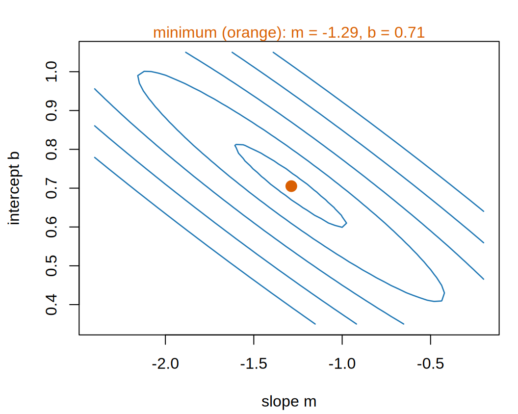
Figure 8: The empirical risk of Equation 10 as a function of the line’s two weights, the slope and the intercept. The marked point is the least-squares fit of Equation 12, where the risk is lowest.
(a) The surface itself (drag to rotate it on the course website). The black lines on it are the contours of the next panel.
(b) The contours of that same surface, shrinking to one point, marked.
Contour lines of the empirical risk, with the slope m from -2.4 to -0.2 on the horizontal axis and the intercept b from 0.35 to 1.05 on the vertical axis, closing in on a single orange point, the least-squares line at slope about -1.29 and intercept about 0.71.
ExrExercise 14 (Read the surface)

Exercise 14 (Read the surface) Equation 11 asks for the lowest point of a surface. For the straight lines of Equation 2 that surface is plotted over two axes, \(m\) and \(b\), and Figure 8 draws it.

How many points on the surface are lower than every other point?

Solution 14. One. The contours shrink to a single point, and every straight-line slice through that point has its minimum there too. That point has lower risk than every other point in the whole plane, so it is the surface’s global minimizer, and \((\hat{m}, \hat{b})\) in Equation 11 is the single element of the argmin.

ExrExercise 15 (Read the surface (part 2))

Exercise 15 (Read the surface (part 2)) Use the setup of Exercise 14.

Would a search for the lowest point give a different answer depending on where it started?

Solution 15. No: the surface has no other local minimizer that a search could stop at, so wherever a search starts it ends at the same point. So both languages in Solution 13 agree without anyone choosing a starting guess.

Squared error and a model linear in its parameters give a surface that is a paraboloid, and a paraboloid has one minimum, and it has a closed-form solution. Neither property holds for most models in the rest of these notes: Gradient Descent starts on what replaces them.

Slide the line in Figure 9 until its empirical risk is as small as you can make it, and watch the dot on the contour map move as you go.

Show code
viewof reM = Inputs.range([-3, 0.5], {width: 360, value: -0.5, step: 0.01, label: "slope m"})
viewof reB = Inputs.range([0, 1.2], {width: 360, value: 0.4, step: 0.005, label: "intercept b"})
viewof reShow = Inputs.checkbox(["least-squares line"], {label: "show"})
Show code
md`Empirical risk of this line: **${reRisk(reM, reB).toFixed(6)}**.
${reShowBest ? `The least-squares line, m = ${reBest.m.toFixed(4)} and b = ${reBest.b.toFixed(4)}, has an empirical risk of ${reRisk(reBest.m, reBest.b).toFixed(6)}.` : ""}`
Show code
Plot.plot({
  ariaLabel: 'The five neighbourhoods, crime rate against per-capita income, ' +
    'with the chosen line drawn in blue ' +
    'and a red segment from each point to the line showing its residual.',
  width: 300, height: 280, grid: true,
  x: {domain: [0, 0.6], label: "per-capita income x"},
  y: {domain: [-0.2, 0.8], label: "crime rate y"},
  marks: [
    Plot.link(biCrime, {x1: (d) => d[0], y1: (d) => d[1], x2: (d) => d[0],
                        y2: (d) => reM * d[0] + reB, stroke: "#d62728", strokeWidth: 2}),
    Plot.line([0, 0.6], {x: (x) => x, y: (x) => reM * x + reB, stroke: "#1f77b4",
                         strokeWidth: 2.5, clip: true}),
    reShowBest ? Plot.line([0, 0.6], {x: (x) => x, y: (x) => reBest.m * x + reBest.b,
                                      stroke: "#555", strokeDasharray: "5,4", clip: true}) : null,
    Plot.dot(biCrime, {x: (d) => d[0], y: (d) => d[1], r: 5, fill: "#222"})
  ]
})
Show code
Plot.plot({
  ariaLabel: 'Contour map of the empirical risk over the slope m and the intercept b, ' +
    'darker where the risk is smaller, ' +
    'with a dot at the chosen line.',
  width: 300, height: 280, marginLeft: 45,
  x: {domain: [-3, 0.5], label: "slope m"},
  y: {domain: [0, 1.2], label: "intercept b"},
  color: {type: "log", scheme: "YlGnBu", reverse: true, label: "empirical risk", legend: true,
          ticks: [0.01, 0.1, 1], tickFormat: (v) => String(v)},
  marks: [
    Plot.contour({x1: -3, y1: 0, x2: 0.5, y2: 1.2, fill: reRisk,
                  thresholds: d3.range(-2.2, 0.01, 0.2).map((e) => 10 ** e),
                  stroke: "#fff", strokeOpacity: 0.4}),
    reShowBest ? Plot.dot([reBest], {x: "m", y: "b", r: 6, symbol: "cross",
                                     stroke: "#d62728", strokeWidth: 2.5}) : null,
    Plot.dot([0], {x: reM, y: reB, r: 5, fill: "#222", stroke: "#fff"})
  ]
})
Figure 9: The empirical risk of Equation 10 for a line you choose, drawn through the five neighborhoods on the left and as a point on the risk surface on the right.
VideosWatch

Lall treats training as minimizing an empirical risk in EE104, from 3:09, and defines the loss, from 5:14 [15], Lecture 6.

2.5 A more flexible model

ExrExercise 16 (Now fit a cubic)

Exercise 16 (Now fit a cubic) Nothing in Equation 8 mentions straight lines. Repeat Exercise 13 with the cubic polynomial

\[ \modmemf{x} = m_3 x^3 + m_2 x^2 + m_1 x + b \tag{13}\]

and report its empirical risk beside the line’s.

Then continue: fit polynomials of degree 2 and 4 as well, and tabulate degree, number of parameters, and empirical risk.
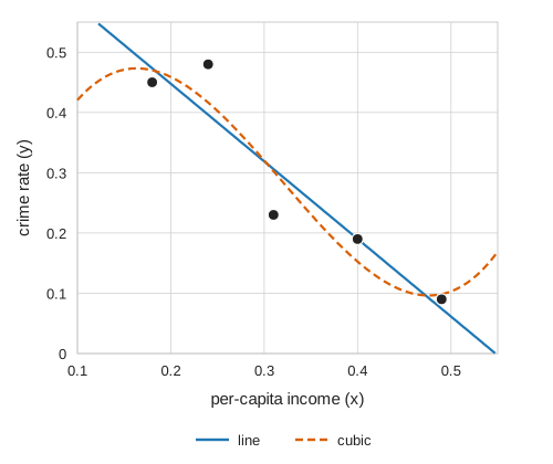
Figure 10: The fitted line of Equation 12 and the cubic fitted in Exercise 16.
Scatterplot of crime rate (vertical axis, 0 to 0.5) against per-capita income (horizontal axis, 0.1 to 0.5) for five neighborhoods. A straight line falling from about 0.45 at income 0.2 to about 0.06 at income 0.5 passes between the points; a dashed cubic curve bends to pass through all five.

Solution 16. Change one argument, and run it over a range of values:

# The five neighbourhoods of @tbl-crime-data, read once in @exm-crime-task.
x <- crime$x
y <- crime$y

for (degree in 1:4) {
  fit <- lm(y ~ poly(x, degree, raw = TRUE))
  risk <- mean(residuals(fit)^2)
  cat(degree, degree + 1, round(risk, 6), "\n")
}
1 2 0.002721 
2 3 0.002608 
3 4 0.002234 
4 5 0 
import numpy as np

# The five neighbourhoods of the crime table, read once in the first example.
x = crime["x"].to_numpy()
y = crime["y"].to_numpy()

for degree in (1, 2, 3, 4):
    coeffs = np.polyfit(x, y, degree)
    risk = np.mean((np.polyval(coeffs, x) - y) ** 2)
    print(degree, degree + 1, round(risk, 6))
1 2 0.002721
2 3 0.002608
3 4 0.002234
4 5 0.0
Show code
# The Python fits again, kept for the equation, the table and the prose.
fits = {degree: np.polyfit(x, y, degree) for degree in (1, 2, 3, 4)}
risks = [float(np.mean((np.polyval(fits[d], x) - y) ** 2)) for d in (1, 2, 3, 4)]
cubic = [float(c) for c in fits[3]]
quartic_max_resid = float(np.max(np.abs(np.polyval(fits[4], x) - y)))
Show code
risks <- py$risks
cubic <- py$cubic
# A signed term of the fitted polynomial, for display math: "- 23.6095\,x^2".
term <- function(coef, power) {
  sign <- if (coef < 0) "-" else "+"
  x <- c("", "\\,x", "\\,x^2", "\\,x^3")[power + 1]
  sprintf("%s %.4f%s", sign, abs(coef), x)
}
e6 <- function(v) sprintf("%.6f", v)
risk_cut <- round(100 * (1 - risks[3] / risks[1]))
# The quartic's risk prints as 0.000000 at six decimals; check that its
# largest residual is below the last printed place, so the table's zero is honest.
max_resid <- py$quartic_max_resid
stopifnot(max_resid < 1e-6)

The cubic comes out at

\[ \emodmemf{x} = 24.6063\,x^3 - 23.6095\,x^2 + 5.7443\,x + 0.0576 \tag{14}\]

and the four fits compare like this:

Table 3: Empirical risk falls monotonically as the model gains parameters. The quartic’s risk is not rounded down: its largest residual on these five points is below 0.000001, the last place the table prints.
degree parameters empirical risk
1 2 0.002721
2 3 0.002608
3 4 0.002234
4 5 0.000000

Two things in Table 3 are worth examining closely.

Among the fits that do not pass through every point, the cubic has the lowest risk, but it improves on the line by very little: \(0.002234\) against \(0.002721\) is a reduction of 18%, obtained by using twice as many parameters. Figure 10 shows what that 18% looks like.

The quartic has the lowest risk, scoring exactly zero. That is not a good model; it is five parameters fitted to five points, so it passes through every one of them by construction and would do so whatever the numbers had been.

VideosWatch

Hastie and Tibshirani compare structured and flexible models [6], video 2.2.

Raise the degree in Figure 11 and watch the empirical risk fall.

Show code
viewof deDegree = Inputs.range([0, 4], {width: 360, value: 1, step: 1, label: "degree"})
Show code
md`A degree-${deDegree} polynomial has ${deDegree + 1} parameter${deDegree === 0 ? "" : "s"}.
Its least-squares fit has empirical risk **${deFit.risk.toFixed(6)}**.`
Show code
Plot.plot({
  ariaLabel: 'The five neighbourhoods, crime rate against per-capita income, ' +
    'with the least-squares polynomial of the chosen degree drawn through them.',
  width: 300, height: 260, grid: true,
  x: {domain: [0.1, 0.55], label: "per-capita income x"},
  y: {domain: [-0.2, 0.8], label: "crime rate y"},
  marks: [
    Plot.line(d3.range(0.1, 0.5501, 0.0025), {x: (x) => x, y: deFit.h,
                                              stroke: "#1f77b4", strokeWidth: 2.5, clip: true}),
    Plot.dot(biCrime, {x: (d) => d[0], y: (d) => d[1], r: 5, fill: "#222"})
  ]
})
Show code
Plot.plot({
  ariaLabel: 'Empirical risk of the least-squares fit for each degree from 0 to 4, ' +
    'on a log scale, as bars, with the chosen degree highlighted.',
  width: 260, height: 260, marginLeft: 80,
  x: {label: "degree", type: "band"},
  y: {type: "log", domain: [1e-8, 0.1], label: "empirical risk (log scale)",
      ticks: biPow10(1e-8, 0.1), tickFormat: biExp},
  marks: [
    Plot.barY(deFits, {x: "degree", y1: 1e-8, y2: (d) => Math.max(d.risk, 1e-8),
                       fill: (d) => d.degree === deDegree ? "#ff7f0e" : "#9ecae1"}),
    Plot.text(deFits.filter((d) => d.risk < 1e-8), {x: "degree", y: 1e-8, text: () => "0",
                                                    dy: -8, fontWeight: "bold"})
  ]
})
Figure 11: Least-squares polynomials of degree 0 to 4 fitted to the five neighborhoods of Table 1, with the empirical risk of each. A degree-4 fit’s risk is zero up to rounding error, which a log scale cannot draw, so its bar is marked 0 instead. The figure has no interval band or interval on the risks: the five neighborhoods are the whole training set, with no sampling model behind them, so each fit and its empirical risk are exact summaries of these five points.
ExrExercise 17 (Which model was actually better?)

Exercise 17 (Which model was actually better?) Table 3 ranks the four fits, and the quartic comes first. Say why that ranking is not a reason to prefer it, and name what you would have to measure instead.

Solution 17. Because the ranking is computed on the very points the models were fitted to. Any flexibility a model has can be used to fit those points closely, so Equation 8 rewards flexibility and accuracy alike and does not distinguish them. The quartic makes that visible by reaching zero: with as many parameters as data points it interpolates, and interpolation is available to it regardless of whether the data has any pattern at all.

What we want is the loss on points the model has not seen. That quantity is the risk (Definition 11), and it can only ever be estimated; the Generalization page says how.

Every honest estimate of it rests on data held out of the fitting.

This is the whole of the bias-variance story in small form, and it is worth noticing that nothing about it is specific to polynomials. Swap in any family whose members can be made arbitrarily flexible and the same thing happens. Hastie et al. [1], Section 2.9, makes the general argument.

DefDefinition 21 (Interpolation)

Definition 21 (Interpolation) A model \(\modmem\) interpolates a data set \(\dataset\) when it predicts every output in \(\dataset\) exactly: \(\modmemf{x_{(i)}} = y_{(i)}\) for each of the \(n\) pairs \((x_{(i)}, y_{(i)})\) of \(\dataset\).

ExmExample 21 (The quartic passes through all five neighborhoods)

Example 21 (The quartic passes through all five neighborhoods) Predict the five neighborhoods of Table 1 with the quartic of Table 3, and compare each prediction with the observed crime rate.

# fits, x and y are the polynomial fits and the five neighbourhoods of @sol-fit-cubic.
quartic_pred = np.polyval(fits[4], x)
print(np.round(quartic_pred, 6))
[0.09 0.45 0.23 0.19 0.48]
print(np.round(y, 6))
[0.09 0.45 0.23 0.19 0.48]

The two rows agree, and the largest residual is 8.7e-14, which is floating-point rounding error. The quartic has five parameters, and the five neighborhoods have distinct inputs, so it can pass through all of them: it interpolates the training set, and its training error under squared-error loss is zero. The line, the quadratic and the cubic have positive training errors in Table 3, so none of them interpolates.

ExrExercise 18 (What we made easy)

Exercise 18 (What we made easy) We took three easy steps in the crime example: we found the lowest point of the risk surface, we chose a model family, and we scored the fitted models. For each step, say what about this example made it easy for us, and what would make it hard on a larger problem.

Solution 18. We made each step easy on purpose, and later chapters remove each simplification.

  • We found the minimum exactly. We can minimize a paraboloid by solving a linear system. We cannot do that for a neural network’s risk surface, so we reduce the risk step by step instead. That is why the derivative of the loss matters so much. Gradient Descent starts on that.

  • We chose the model by eye. Five points and one input let us look at the scatter plot. With many inputs there is nothing to look at, so we have to argue for the choice of family and then check it.

  • We computed the score on the training data. Solution 17 says why that is not a measurement of anything we care about. The Generalization page says what to do instead.

Reading

VideosWatch

The Data Science Learning Community’s book clubs discuss An Introduction to Statistical Learning, Chapter 2, in recorded meetings:

Dependency graph

Open the block to see every definition and result of this page, with prerequisites at the top. Click a box to jump to it.

Definitions on this page

References

[1]
T. Hastie, R. Tibshirani, and J. Friedman, The elements of statistical learning: Data mining, inference, and prediction, 2nd ed. Springer, 2009. Available: https://hastie.su.domains/ElemStatLearn/
[2]
G. James, D. Witten, T. Hastie, and R. Tibshirani, An introduction to statistical learning with applications in R, 2nd ed. Springer, 2021. Available: https://www.statlearning.com/
[3]
B. Hutchinson, “DATA 471/571: Machine learning.” Western Washington University, 2025.
[4]
Wikipedia contributors, “Training, validation, and test data sets — Wikipedia, the free encyclopedia.” 2026. Available: https://en.wikipedia.org/wiki/Training,_validation,_and_test_data_sets
[5]
Wikipedia contributors, “Parametric model — Wikipedia, the free encyclopedia.” 2026. Available: https://en.wikipedia.org/wiki/Parametric_model
[6]
T. Hastie, R. Tibshirani, and J. Taylor, “Statistical learning with python.” Stanford Online, lecture videos on YouTube, 2023. Available: https://www.youtube.com/playlist?list=PLoROMvodv4rPP6braWoRt5UCXYZ71GZIQ
[7]
Wikipedia contributors, “Loss function — Wikipedia, the free encyclopedia.” 2026. Available: https://en.wikipedia.org/wiki/Loss_function
[8]
Y. S. Abu-Mostafa, M. Magdon-Ismail, and H.-T. Lin, Learning from data: A short course. AMLBook, 2012. Available: https://amlbook.com/
[9]
Wikipedia contributors, “Empirical risk minimization — Wikipedia, the free encyclopedia.” 2026. Available: https://en.wikipedia.org/wiki/Empirical_risk_minimization
[10]
B. Hutchinson, “DATA 471/571 (machine learning) and CSCI 481/581 (deep learning) video lectures.” Western Washington University. Accessed: Sep. 28, 2026. [Online]. Available: https://facultyweb.cs.wwu.edu/~hutchib2/video_lectures/data371/
[11]
GeeksforGeeks, “ML | common loss functions.” GeeksforGeeks, tutorial article, 2025. Available: https://www.geeksforgeeks.org/machine-learning/ml-common-loss-functions/
[12]
GeeksforGeeks, “Empirical risk minimization.” GeeksforGeeks, tutorial article, 2025. Available: https://www.geeksforgeeks.org/machine-learning/empirical-risk-minimization/
[13]
Wikipedia contributors, “Evaluation of binary classifiers — Wikipedia, the free encyclopedia.” 2026. Available: https://en.wikipedia.org/wiki/Evaluation_of_binary_classifiers
[14]
U. von Luxburg, “Statistical machine learning.” University of Tübingen, lecture videos on YouTube, 2020. Available: https://www.youtube.com/playlist?list=PL05umP7R6ij2XCvrRzLokX6EoHWaGA2cC
[15]
S. Lall, “EE104: Introduction to machine learning, 2020.” Stanford Online, lecture videos on YouTube, 2020. Available: https://www.youtube.com/playlist?list=PLoROMvodv4rN_Uy7_wmS051_q1d6akXmK
[16]
T. M. Mitchell, Machine learning. in McGraw-hill series in computer science. New York: McGraw-Hill, 1997.
[17]
Data Science Learning Community, “Introduction to statistical learning using R (islr06).” Book club meeting recordings on YouTube, 2023. Available: https://www.youtube.com/playlist?list=PL3x6DOfs2NGjlhpKMiWsDcKL2nngwXROq
[18]
Data Science Learning Community, “Introduction to statistical learning using Python (islp03).” Book club meeting recordings on YouTube, 2025. Available: https://www.youtube.com/playlist?list=PL3x6DOfs2NGgbSNh0UG87rrM-z5LiKLZp
Back to top