Nonparametric Models
1 Empirical CDF
2 Order statistics
3 Sample quantiles
The CDF \(F\) and the quantile function \(Q\) describe a probability distribution, while \(\hat F\) and \(\hat Q\) describe a sample, and serve as estimates of \(F\) and \(Q\).
Proof. Fix \(p\) with \((i-1)/n < p \le i/n\).
For any \(t < x_{(i)}\), the \(n - i + 1\) values \(x_{(i)}, \ldots, x_{(n)}\) all exceed \(t\), so at most \(i - 1\) values are at most \(t\), and:
\[ \begin{aligned} \hat F(t) &\le \frac{i-1}{n} && \text{(at most $i - 1$ indicators equal 1)}\\ &< p && \text{(choice of $p$)} \end{aligned} \]
So no \(t < x_{(i)}\) belongs to the set \(\mathopen{}\left\{t : \hat F(t) \ge p\right\}\mathclose{}\).
At \(t = x_{(i)}\), the \(i\) values \(x_{(1)}, \ldots, x_{(i)}\) are all at most \(x_{(i)}\), so:
\[ \begin{aligned} \hat F\mathopen{}\left(x_{(i)}\right)\mathclose{} &\ge \frac{i}{n} && \text{(at least $i$ indicators equal 1)}\\ &\ge p && \text{(choice of $p$)} \end{aligned} \]
So \(x_{(i)}\) belongs to the set, and it is the smallest member of the set, because no smaller \(t\) belongs to it. Therefore \(\hat Q(p) = x_{(i)}\).
Other sources, and other software defaults, define sample quantiles differently, mostly by interpolating between order statistics. R’s quantile() offers nine definitions through its type argument, and its default (type = 7) interpolates, so quantile(c(4, 1, 7, 3), 0.5) returns 3.5, not 3. The usual sample median is another interpolated quantile: for an even number of observations, it averages the two middle order statistics. These notes use Definition 3, which always returns one of the observed values.
4 The empirical CDF and quantile function as generalized inverses
Show R code
x <- c(4, 1, 7, 3)
n <- length(x)
x_ord <- sort(x)
p_ord <- seq_len(n) / n
ecdf_x_padding <- 0.8
x_min <- min(x_ord) - ecdf_x_padding
x_max <- max(x_ord) + ecdf_x_padding

x_left <- c(x_min, x_ord)
x_right <- c(x_ord, x_max)
f_levels <- c(0, p_ord)

plot(
  0,
  0,
  type = "n",
  xlim = c(x_min, x_max),
  ylim = c(0, 1.05),
  xlab = "t",
  ylab = expression(hat(plain("F"))(t))
)
segments(x_left, f_levels, x_right, f_levels, lwd = 2, col = "blue")
points(x_ord, f_levels[seq_len(n)], pch = 1, col = "blue")
points(x_ord, f_levels[seq_len(n) + 1], pch = 19, col = "blue")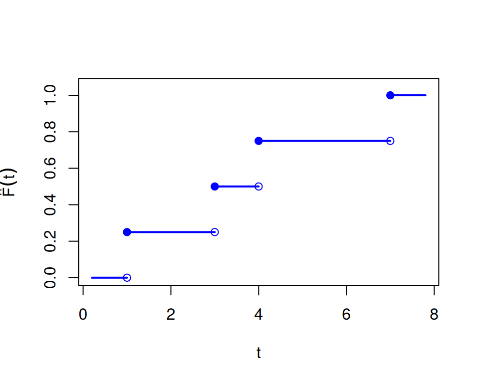
Show R code
eqf_y_padding <- 0.5
q_left <- c(0, p_ord[-n])
q_right <- p_ord
plot(
  0,
  0,
  type = "n",
  xlim = c(0, 1),
  ylim = c(min(x_ord) - eqf_y_padding, max(x_ord) + eqf_y_padding),
  xlab = "p",
  ylab = expression(hat(Q)(p))
)
segments(q_left, x_ord, q_right, x_ord, lwd = 2, col = "blue")
points(q_left, x_ord, pch = 1, col = "blue")
points(q_right, x_ord, pch = 19, col = "blue")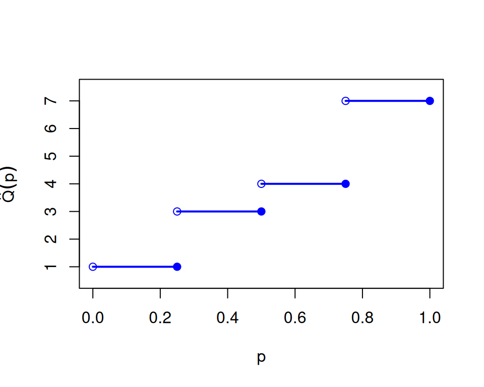
Both functions in Figure 1 are step functions, so neither is one-to-one. Each flat piece of one function corresponds to a jump of the other: for example, \(\hat F(t) = 0.5\) for every \(t \in [3, 4)\), and \(\hat Q\) jumps from 3 to 4 at \(p = 0.5\). So \(\hat Q\) is a generalized inverse of \(\hat F\), not an inverse in the usual sense: \(\hat Q(\hat F(t)) \le t\) for every \(t \ge x_{(1)}\), with equality only at the observed values.