The Bootstrap

Published

Last modified: 2026-09-29 00:05:17 (PDT)

This page reviews the bootstrap, a resampling method for standard errors and confidence intervals that does not need a formula for the sampling distribution of a statistic. Its HERS example bootstraps the slope of a simple linear regression. This page is adapted from Vittinghoff et al. (2012), Section 3.6.

1 The HERS data

The examples on this page use the HERS data, which the Comparing Means page describes. The rmb R package includes the dataset; haven::as_factor() converts its Stata value labels to factors:

hers <- rmb::hers |> haven::as_factor()

2 Bootstrap confidence intervals

2.1 When to use the bootstrap

The bootstrap (Efron 1979; Efron and Tibshirani 1993) estimates the sampling distribution of a statistic by resampling the observed data. It gives standard errors and confidence intervals in three situations where the usual formulas fall short (Vittinghoff et al. 2012, chap. 3):

approximate methods for valid confidence intervals exist, but standard software does not implement them conveniently;
no closed-form approximate method has been found;
the data violate the assumptions of the established methods badly enough that their confidence intervals would be unreliable.

2.2 The bootstrap procedure

Definition 1 (Bootstrap sample) A bootstrap sample from observed data \(x_1, \ldots, x_n\) is a sample of size \(n\) drawn with replacement from \(\mathopen{}\left\{x_1, \ldots, x_n\right\}\mathclose{}\), each draw choosing each of the \(n\) observations with probability \(1/n\).

Because the draws are with replacement, a bootstrap sample usually contains some observations more than once and omits others.

Example 1 (Bootstrap samples of five glucose values) Take the baseline fasting glucose values of the first five HERS participants, and draw two bootstrap samples from them:

glucose5 <- hers$glucose[1:5]
glucose5
#> [1]  84 111 114  94 101
set.seed(1)
list(
  sample_1 = sample(glucose5, replace = TRUE),
  sample_2 = sample(glucose5, replace = TRUE)
)
#> $sample_1
#> [1]  84  94  84 111 101
#> 
#> $sample_2
#> [1] 114 111 114 114  84

Each bootstrap sample has five values, but some original values appear more than once and others do not appear at all.

Definition 2 (Bootstrap distribution) Let \(\hat\theta\) be a statistic computed from the observed data. Draw \(B\) independent bootstrap samples, and compute the statistic on each one, giving \(\hat\theta^*_1, \ldots, \hat\theta^*_B\). The bootstrap distribution of \(\hat\theta\) is the empirical distribution of \(\hat\theta^*_1, \ldots, \hat\theta^*_B\).

The bootstrap distribution estimates the sampling distribution of \(\hat\theta\). The observed sample stands in for the population, and resampling from it stands in for drawing new samples from the population.

Definition 3 (Bootstrap standard error) The bootstrap standard error of a statistic \(\hat\theta\), written \(\widehat{\text{SE}}_\text{boot}\), is the sample standard deviation of the bootstrap replicates \(\hat\theta^*_1, \ldots, \hat\theta^*_B\) (Definition 2). It estimates the standard error of \(\hat\theta\).

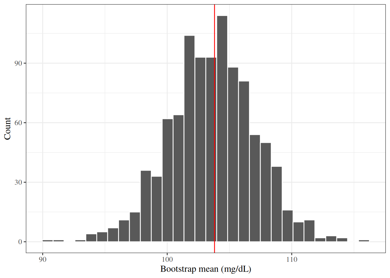
Example 2 (Bootstrap distribution of a mean of ten glucose values) Take the baseline fasting glucose values of the first ten HERS participants, and compute the sample mean of each of \(B = 1{,}000\) bootstrap samples:

glucose10 <- hers$glucose[1:10]
set.seed(42)
boot_means10 <- replicate(1000, mean(sample(glucose10, replace = TRUE)))
c(
  observed_mean = mean(glucose10),
  bootstrap_se = sd(boot_means10),
  formula_se = sd(glucose10) / sqrt(10),
  divide_by_n_se = sqrt(mean((glucose10 - mean(glucose10))^2) / 10)
)
#>  observed_mean   bootstrap_se     formula_se divide_by_n_se 
#>      103.80000        3.47992        3.61417        3.42870

The bootstrap standard error (Definition 3) is close to the usual estimate \(s / \sqrt{n}\). Each bootstrap draw has variance \(\hat\sigma^2 \stackrel{\text{def}}{=}\frac{1}{n} \sum_{i=1}^n (x_i - \bar{x})^2\) around \(\bar{x}\), and the \(n\) draws are independent, so as \(B\) grows the bootstrap standard error of the mean approaches \(\hat\sigma / \sqrt{n}\) (divide_by_n_se), which is smaller than \(s / \sqrt{n}\) by the factor \(\sqrt{(n-1)/n}\). Figure 1 shows the bootstrap distribution.

Show R code

tibble::tibble(mean = boot_means10) |>
  ggplot2::ggplot() +
  ggplot2::aes(x = mean) +
  ggplot2::geom_histogram(bins = 30, color = "white") +
  ggplot2::geom_vline(xintercept = mean(glucose10), color = "red") +
  ggplot2::labs(x = "Bootstrap mean (mg/dL)", y = "Count")

Figure 1: Bootstrap distribution of the mean fasting glucose of the first ten HERS participants (\(B = 1{,}000\)). The red line marks the observed mean.

2.3 Bootstrap confidence interval methods

There are three common methods for turning a bootstrap distribution into a \(100(1-\alpha)\%\) confidence interval for a parameter \(\theta\) (Vittinghoff et al. 2012, chap. 3; Efron and Tibshirani 1993). Each is an approximate confidence interval. Throughout, \(z_q\) is the \(q\) quantile of the standard Gaussian distribution and \(\Phi\) is its CDF.

2.3.1 Normal approximation

Definition 4 (Normal bootstrap confidence interval) The normal bootstrap confidence interval is

\[\hat\theta \pm z_{1 - \alpha/2} \, \widehat{\text{SE}}_\text{boot},\]

where \(\widehat{\text{SE}}_\text{boot}\) is the bootstrap standard error (Definition 3).

This interval assumes that the sampling distribution of \(\hat\theta\) is approximately Gaussian and centered at \(\theta\), so it can be unreliable when that distribution is skewed. It needs only a standard error, which takes fewer bootstrap replicates to estimate well than the tail quantiles used by the next two intervals (Efron and Tibshirani 1993).

Example 3 (Normal bootstrap interval for the mean of ten glucose values) Continuing Example 2, the 95% interval of Definition 4 is:

mean(glucose10) +
  c(lower = -1, upper = 1) * qnorm(0.975) * sd(boot_means10)
#>    lower    upper 
#>  96.9795 110.6205

2.3.2 Percentile method

Definition 5 (Percentile bootstrap confidence interval) The percentile bootstrap confidence interval runs from the \(\alpha/2\) quantile to the \(1 - \alpha/2\) quantile of the bootstrap replicates \(\hat\theta^*_1, \ldots, \hat\theta^*_B\) (Definition 2).

The extreme quantiles of \(B\) replicates are noisy estimates, so percentile-based intervals need more replicates than the normal interval; \(B\) of at least \(1{,}000\) is a common choice.

Example 4 (Percentile bootstrap interval for the mean of ten glucose values) Continuing Example 2, the 95% interval of Definition 5 is:

quantile(boot_means10, c(0.025, 0.975))
#>  2.5% 97.5% 
#>  96.5 110.4

2.3.3 Bias-corrected and accelerated method

Definition 6 (Bias correction of the BCa interval) For a statistic \(\hat\theta\) and its bootstrap replicates \(\hat\theta^*_1, \ldots, \hat\theta^*_B\), the bias correction is

\[\hat{z}_0 \stackrel{\text{def}}{=}\Phi^{-1}\mathopen{}\left(\frac{\#\mathopen{}\left\{b : \hat\theta^*_b < \hat\theta\right\}\mathclose{}}{B}\right)\mathclose{},\]

where \(\Phi\) is the standard Gaussian CDF.

Example 5 (Bias correction when 40% of replicates fall below the estimate) If 400 of \(B = 1{,}000\) replicates are below \(\hat\theta\), then \(\hat z_0 = \Phi^{-1}(0.4) \approx -0.253\). If exactly half were below, \(\hat z_0 = \Phi^{-1}(0.5) = 0\).

Definition 7 (Acceleration of the BCa interval) Let \(\hat\theta_{(i)}\) be the statistic computed with observation \(i\) deleted, and let \(\hat\theta_{(\cdot)}\) be the mean of \(\hat\theta_{(1)}, \ldots, \hat\theta_{(n)}\). The acceleration is

\[\hat{a} \stackrel{\text{def}}{=}\frac{\sum_{i=1}^n \mathopen{}\left(\hat\theta_{(\cdot)} - \hat\theta_{(i)}\right)\mathclose{}^3} {6 \mathopen{}\left(\sum_{i=1}^n \mathopen{}\left(\hat\theta_{(\cdot)} - \hat\theta_{(i)}\right)\mathclose{}^2\right)\mathclose{}^{3/2}}.\]

Example 6 (Acceleration from three deleted estimates) If the differences \(\hat\theta_{(\cdot)} - \hat\theta_{(i)}\) are \(1\), \(1\), and \(-2\), the sum of their cubes is \(1 + 1 - 8 = -6\) and the sum of their squares is \(6\), so

\[\hat a = \frac{-6}{6 \cdot 6^{3/2}} \approx -0.068.\]

Definition 8 (Bias-corrected and accelerated bootstrap confidence interval) With the bias correction \(\hat z_0\) and the acceleration \(\hat a\), for \(q \in \mathopen{}\left\{\alpha/2, 1 - \alpha/2\right\}\mathclose{}\), let

\[\alpha_q \stackrel{\text{def}}{=}\Phi\mathopen{}\left(\hat{z}_0 + \frac{\hat{z}_0 + z_q}{1 - \hat{a}(\hat{z}_0 + z_q)}\right)\mathclose{}.\]

The bias-corrected and accelerated (BCa) bootstrap confidence interval runs from the \(\alpha_{\alpha/2}\) quantile to the \(\alpha_{1 - \alpha/2}\) quantile of the bootstrap replicates (Efron and Tibshirani 1993, chap. 14).

When \(\hat{z}_0 = 0\) and \(\hat{a} = 0\), \(\alpha_q = q\) and the BCa interval is the percentile interval (Definition 5). \(\hat{z}_0\) measures how far the bootstrap distribution’s median sits from \(\hat\theta\), and \(\hat{a}\) measures its skewness, so the BCa interval shifts the percentile interval to correct for both.

Example 7 (BCa bootstrap interval for the mean of ten glucose values) Continuing Example 2, the quantities of Definition 8, step by step:

z0 <- qnorm(mean(boot_means10 < mean(glucose10)))
jackknife_means <- vapply(1:10, \(i) mean(glucose10[-i]), numeric(1))
dev <- mean(jackknife_means) - jackknife_means
a_hat <- sum(dev^3) / (6 * sum(dev^2)^(3 / 2))
z_q <- qnorm(c(0.025, 0.975))
alpha_q <- pnorm(z0 + (z0 + z_q) / (1 - a_hat * (z0 + z_q)))
c(z_0 = z0, a_hat = a_hat, alpha_lower = alpha_q[1], alpha_upper = alpha_q[2])
#>         z_0       a_hat alpha_lower alpha_upper 
#>  0.01002668 -0.00867722  0.02422093  0.97422713
quantile(boot_means10, alpha_q)
#> 2.422093% 97.42271% 
#>      96.5     110.4

The acceleration \(\hat{a}\) is nearly 0 here, and \(\hat{z}_0\) is small, so the BCa interval is close to the percentile interval of Example 4.

2.4 The boot package

The boot package (Davison and Hinkley 1997), a recommended package distributed with R, provides boot::boot() to draw the bootstrap replicates and boot::boot.ci() to compute the three intervals. boot::boot.ci() differs from the definitions on this page in two small ways:

its normal interval (type = "norm") is centered at \(\hat\theta\) minus the bootstrap estimate of bias, \(\hat\theta - (\bar\theta^* - \hat\theta)\), where \(\bar\theta^*\) is the mean of the replicates, rather than at \(\hat\theta\);
it estimates quantiles of the replicates by interpolation, so its percentile and BCa endpoints can differ slightly from those computed with quantile().

2.5 Example: slope of SBP on age in HERS

Example 8 (Bootstrap confidence intervals for the slope of SBP on age in HERS) We regress systolic blood pressure (SBP) on age by ordinary least squares, and bootstrap the slope, resampling participants (adapted from Vittinghoff et al. 2012, chap. 3). The statistic function takes the data and the row indices of one bootstrap sample:

slope_sbp_age <- function(data, indices) {
  fit <- lm(SBP ~ age, data = data[indices, ])
  coef(fit)[["age"]]
}

set.seed(42)
boot_result <- boot::boot(data = hers, statistic = slope_sbp_age, R = 1000)
boot_result
#> 
#> ORDINARY NONPARAMETRIC BOOTSTRAP
#> 
#> 
#> Call:
#> boot::boot(data = hers, statistic = slope_sbp_age, R = 1000)
#> 
#> 
#> Bootstrap Statistics :
#>     original       bias    std. error
#> t1* 0.471728 -0.000635537   0.0536514

The bootstrap standard error is close to the model-based standard error from lm(), and the three bootstrap intervals are close to the model-based 95% confidence interval:

fit_sbp_age <- lm(SBP ~ age, data = hers)
summary(fit_sbp_age)$coefficients["age", ]
#>    Estimate  Std. Error     t value    Pr(>|t|) 
#> 4.71728e-01 5.36838e-02 8.78716e+00 2.64196e-18
confint(fit_sbp_age)["age", ]
#>    2.5 %   97.5 % 
#> 0.366464 0.576993
boot::boot.ci(boot_result, type = c("norm", "perc", "bca"))
#> BOOTSTRAP CONFIDENCE INTERVAL CALCULATIONS
#> Based on 1000 bootstrap replicates
#> 
#> CALL : 
#> boot::boot.ci(boot.out = boot_result, type = c("norm", "perc", 
#>     "bca"))
#> 
#> Intervals : 
#> Level      Normal             Percentile            BCa          
#> 95%   ( 0.3672,  0.5775 )   ( 0.3607,  0.5811 )   ( 0.3624,  0.5824 )  
#> Calculations and Intervals on Original Scale

All three intervals are similar here. When the bootstrap distribution is skewed, the intervals differ more, and the BCa interval, which corrects for skewness, is the better choice (Efron and Tibshirani 1993, chap. 14).

References

Davison, Anthony C., and David V. Hinkley. 1997. Bootstrap Methods and Their Application. Cambridge Series in Statistical and Probabilistic Mathematics 1. Cambridge University Press. https://doi.org/10.1017/CBO9780511802843.

Efron, Bradley. 1979. “Bootstrap Methods: Another Look at the Jackknife.” The Annals of Statistics 7 (1): 1–26. https://doi.org/10.1214/aos/1176344552.

Efron, Bradley, and Robert J. Tibshirani. 1993. An Introduction to the Bootstrap. Monographs on Statistics and Applied Probability 57. Chapman & Hall/CRC. https://doi.org/10.1201/9780429246593.

Vittinghoff, Eric, David V Glidden, Stephen C Shiboski, and Charles E McCulloch. 2012. Regression Methods in Biostatistics: Linear, Logistic, Survival, and Repeated Measures Models. 2nd ed. Springer. https://doi.org/10.1007/978-1-4614-1353-0.