Comparing Means

1 Introduction

This page reviews the standard methods for comparing the mean of a continuous outcome between groups: t-tests, confidence intervals for a difference in means, and one-way analysis of variance.

This page builds on three others:

• Exploratory Data Analysis defines the sample statistics these methods use;
• Statistical Inference defines hypotheses, test statistics, p-values, confidence intervals, and the t, chi-square, and F reference distributions;
• Estimation defines estimators and their standard errors.

The t-tests and ANOVA on this page are the exact, Gaussian-outcome tests in the table of exact and approximate tests on the Maximum Likelihood page, which pairs each one with its large-sample counterpart.

This page is adapted from Vittinghoff et al. (2012), Chapter 3.

2 The HERS data

The “heart and estrogen/progestin study” (HERS) was a clinical trial of hormone therapy for prevention of recurrent heart attacks and death among 2,763 post-menopausal women with existing coronary heart disease (CHD) (Hulley et al. 1998).

The trial was conducted at 20 US clinical centers. Participants were randomized to receive either conjugated equine estrogens (0.625 mg/day) plus medroxyprogesterone acetate (2.5 mg/day) or a matching placebo (Hulley et al. 1998). Women were followed for an average of 4.1 years (Hulley et al. 1998).

The primary outcome was nonfatal myocardial infarction or CHD death (Hulley et al. 1998).

The HERS data are distributed with Vittinghoff et al. (2012) on the book’s companion website, as a Stata file that R can read directly:

# one unbroken string, so that link checkers test the whole URL:
url <- "https://regression.ucsf.edu/sites/g/files/tkssra16191/files/wysiwyg/home/data/hersdata.dta" # nolint: line_length_linter.
hers <- haven::read_dta(url)

The rmb R package includes the same file, which these notes use so that rendering does not depend on the website. haven::as_factor() converts the Stata value labels to factors:

hers <- rmb::hers |> haven::as_factor()

The examples on this page use these variables:

Variable	Meaning
HT	Randomized treatment: placebo or hormone therapy
age	Age at baseline (years)
raceth	Race/ethnicity: White, African American, or Other
exercise	Exercises at least three times per week (no/yes)
BMI	Body mass index at baseline (kg/m2)
SBP	Systolic blood pressure at baseline (mmHg)
glucose	Fasting glucose at baseline (mg/dL)
glucose1	Fasting glucose at the year-1 visit (mg/dL)

hers |>
  dplyr::select(HT, age, raceth, exercise, BMI, SBP, glucose, glucose1) |>
  dplyr::glimpse()
#> Rows: 2,763
#> Columns: 8
#> $ HT       <fct> placebo, placebo, hormone therapy, placebo, placebo, hormone …
#> $ age      <dbl> 70, 62, 69, 64, 65, 68, 70, 69, 61, 62, 72, 73, 52, 57, 57, 6…
#> $ raceth   <fct> African American, African American, White, White, White, Afri…
#> $ exercise <fct> no, no, no, no, no, no, no, yes, yes, no, no, no, no, no, yes…
#> $ BMI      <dbl> 23.69, 28.62, 42.51, 24.39, 21.90, 29.05, 34.45, 23.16, 30.26…
#> $ SBP      <dbl> 138, 118, 134, 152, 175, 174, 119, 178, 162, 111, 122, 158, 1…
#> $ glucose  <dbl> 84, 111, 114, 94, 101, 116, 120, 95, 105, 98, 111, 95, 97, 10…
#> $ glucose1 <dbl> 94, 78, 98, 93, 92, 115, NA, 95, 113, 98, 96, 107, 90, 100, 1…

3 Descriptive statistics

The Exploratory Data Analysis page defines the sample statistics used on this page, each with an example:

• the sample mean;
• the sample median;
• the sample variance;
• the sample standard deviation;
• the interquartile range;
• the sample proportion.

That page also defines the graphs used here, including box plots and scatter plots.

Example 1 (HERS baseline characteristics by treatment group) Table 1 summarizes the HERS participants at baseline, separately for each randomized group. Continuous variables are summarized by mean (standard deviation), and categorical variables by count (percent).

hers |>
  dplyr::select(
    age, BMI, glucose, SBP, DBP,
    HT, raceth, exercise, smoking, diabetes
  ) |>
  gtsummary::tbl_summary(
    by = HT,
    statistic = list(
      gtsummary::all_continuous() ~ "{mean} ({sd})",
      gtsummary::all_categorical() ~ "{n} ({p}%)"
    ),
    digits = gtsummary::all_continuous() ~ 1,
    label = list(
      age ~ "Age (years)",
      BMI ~ "BMI (kg/m^2)",
      glucose ~ "Fasting glucose (mg/dL)",
      SBP ~ "Systolic BP (mmHg)",
      DBP ~ "Diastolic BP (mmHg)",
      raceth ~ "Race/ethnicity",
      exercise ~ "Exercises regularly",
      smoking ~ "Current smoker",
      diabetes ~ "Diabetes"
    )
  ) |>
  gtsummary::add_overall() |>
  gtsummary::bold_labels()

Table 1: HERS: baseline characteristics by treatment group

Characteristic	Overall N = 2,7631	placebo N = 1,3831	hormone therapy N = 1,3801
Age (years)	66.6 (6.7)	66.8 (6.7)	66.5 (6.6)
BMI (kg/m^2)	28.6 (5.5)	28.5 (5.5)	28.6 (5.5)
Unknown	5	4	1
Fasting glucose (mg/dL)	112.2 (36.8)	112.4 (36.8)	111.9 (36.9)
Systolic BP (mmHg)	135.1 (19.0)	135.1 (19.4)	135.0 (18.7)
Diastolic BP (mmHg)	73.2 (9.7)	73.1 (9.7)	73.2 (9.7)
Unknown	1	1	0
Race/ethnicity
White	2,451 (89%)	1,239 (90%)	1,212 (88%)
African American	218 (7.9%)	102 (7.4%)	116 (8.4%)
Other	94 (3.4%)	42 (3.0%)	52 (3.8%)
Exercises regularly	1,068 (39%)	530 (38%)	538 (39%)
Current smoker	360 (13%)	182 (13%)	178 (13%)
Diabetes	731 (26%)	352 (25%)	379 (27%)
1 Mean (SD); n (%)

Because treatment was assigned at random, the two groups differ at baseline only by chance, and their summaries are close.

4 Comparing two groups: continuous outcomes

4.1 Hypotheses

The Statistical Inference page defines the null hypothesis, the alternative hypothesis, test statistics, p-values, and significance levels. In a comparison of two groups with means \(\mu_1\) and \(\mu_2\), the null hypothesis is usually \(H_0: \mu_1 = \mu_2\), and the two-sided alternative is \(H_1: \mu_1 \neq \mu_2\).

4.2 One-sample t-test

Definition 1 (One-sample t-test) Let \(x_1, \ldots, x_n\) be observations with \(n \ge 2\), sample mean \(\bar{x}\), and sample standard deviation \(s\). The one-sample t-test of \(H_0: \mu = \mu_0\) against \(H_1: \mu \neq \mu_0\) uses the statistic

\[t \stackrel{\text{def}}{=}\frac{\bar{x} - \mu_0}{s / \sqrt{n}}.\]

Its p-value is \(\Pr(\mathopen{}\left|T\right|\mathclose{} \ge \mathopen{}\left|t\right|\mathclose{})\), where \(T\) has the \(t_{n-1}\) distribution (t-distribution).

Theorem 1 (Null distribution of the one-sample t statistic) Let \(X_1, \ldots, X_n\) be independent, each Gaussian with mean \(\mu_0\) and variance \(\sigma^2\), with \(n \ge 2\). Then the statistic \(T \stackrel{\text{def}}{=}(\bar X - \mu_0) / (S / \sqrt{n})\) of Definition 1, computed from these random variables, has the \(t_{n-1}\) distribution.

ProofProof

Proof. We use a standard fact about Gaussian samples (Hogg et al. 2019, sec. 5.5, pp. 203-205): \(\bar X\) and \(S^2\) are independent, and \(V \stackrel{\text{def}}{=}(n-1) S^2 / \sigma^2\) has the \(\chi^2_{n-1}\) distribution. Also, \(Z \stackrel{\text{def}}{=}(\bar X - \mu_0) / (\sigma / \sqrt{n})\) has the standard Gaussian distribution, and \(Z\) is independent of \(V\) because \(\bar X\) is independent of \(S^2\). So by the definition of the t-distribution, \(Z / \sqrt{V / (n-1)}\) has the \(t_{n-1}\) distribution, and this ratio equals \(T\):

\[ \begin{aligned} \frac{Z}{\sqrt{V/(n-1)}} &= \frac{(\bar X - \mu_0) / (\sigma / \sqrt{n})}{\sqrt{S^2 / \sigma^2}} && \text{(substitute $Z$ and $V$)}\\ &= \frac{(\bar X - \mu_0) / (\sigma / \sqrt{n})}{S / \sigma} && \text{($\sqrt{S^2} = S$, since $S \ge 0$)}\\ &= \frac{\bar X - \mu_0}{S / \sqrt{n}} && \text{(the factors of $\sigma$ cancel)}\\ &= T. \end{aligned} \]

When the observations are not Gaussian, \(T\) still has approximately the standard Gaussian distribution when \(n\) is large, by the central limit theorem, and then \(t_{n-1}\) is close to the standard Gaussian distribution (t quantiles approach Gaussian quantiles).

4.3 Paired t-test

Definition 2 (Paired t-test) Let \((x_{1,1}, x_{1,2}), \ldots, (x_{n,1}, x_{n,2})\) be pairs of related measurements, such as the same participants measured at two times, and let \(d_i \stackrel{\text{def}}{=}x_{i,2} - x_{i,1}\) be the within-pair differences, with population mean \(\mu_d\). The paired t-test of \(H_0: \mu_d = 0\) against \(H_1: \mu_d \neq 0\) is the one-sample t-test (Definition 1) of \(H_0: \mu = 0\) applied to \(d_1, \ldots, d_n\).

Example 2 (Change in fasting glucose over the first year of HERS) We test whether mean fasting glucose changed between baseline (glucose) and the year-1 visit (glucose1), across both treatment groups. Participants missing either measurement are dropped. The t statistic of Definition 1, computed on the differences:

glucose_change <- hers |>
  dplyr::filter(!is.na(glucose), !is.na(glucose1)) |>
  dplyr::mutate(d = glucose1 - glucose) |>
  dplyr::pull(d)
n_pairs <- length(glucose_change)
t_paired <- mean(glucose_change) / (sd(glucose_change) / sqrt(n_pairs))
c(
  n = n_pairs,
  mean_change = mean(glucose_change),
  t = t_paired,
  p_value = 2 * pt(-abs(t_paired), df = n_pairs - 1)
)
#>           n mean_change           t     p_value 
#> 2.61300e+03 2.62036e+00 4.15081e+00 3.41911e-05

t.test() with paired = TRUE gives the same statistic, along with a confidence interval for \(\mu_d\):

t.test(hers$glucose1, hers$glucose, paired = TRUE)
#> 
#>  Paired t-test
#> 
#> data:  hers$glucose1 and hers$glucose
#> t = 4.151, df = 2612, p-value = 3.42e-05
#> alternative hypothesis: true mean difference is not equal to 0
#> 95 percent confidence interval:
#>  1.38248 3.85824
#> sample estimates:
#> mean difference 
#>         2.62036

Mean fasting glucose rose by about 2.6 mg/dL over the year, and the p-value is far below 0.05.

4.4 Two-sample t-tests

Definition 3 (Welch’s two-sample t-test) Let two independent groups have sample sizes \(n_1, n_2 \ge 2\), sample means \(\bar{x}_1\) and \(\bar{x}_2\), and sample variances \(s_1^2\) and \(s_2^2\). Welch’s two-sample t-test of \(H_0: \mu_1 = \mu_2\) against \(H_1: \mu_1 \neq \mu_2\) uses the statistic

\[t \stackrel{\text{def}}{=}\frac{\bar{x}_1 - \bar{x}_2}{\sqrt{\dfrac{s_1^2}{n_1} + \dfrac{s_2^2}{n_2}}}\]

and the Welch–Satterthwaite degrees of freedom

\[\hat\nu \stackrel{\text{def}}{=}\frac{\mathopen{}\left(\dfrac{s_1^2}{n_1} + \dfrac{s_2^2}{n_2}\right)\mathclose{}^2} {\dfrac{(s_1^2 / n_1)^2}{n_1 - 1} + \dfrac{(s_2^2 / n_2)^2}{n_2 - 1}}.\]

Its p-value is \(\Pr(\mathopen{}\left|T\right|\mathclose{} \ge \mathopen{}\left|t\right|\mathclose{})\), where \(T\) has the \(t_{\hat\nu}\) distribution (t-distribution).

Welch’s test does not assume that the two groups have equal variances. Even for Gaussian data, \(t_{\hat\nu}\) is only an approximation to the null distribution of \(t\). For large groups, the central limit theorem makes the statistic approximately standard Gaussian under \(H_0\), as in the WCGS cholesterol example. Welch’s test is the default in R’s t.test().

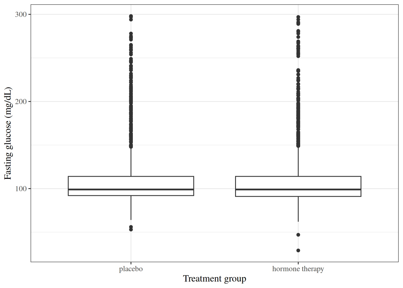
Example 3 (Baseline fasting glucose by treatment group in HERS) We test \(H_0: \mu_\text{HT} = \mu_\text{placebo}\) against \(H_1: \mu_\text{HT} \neq \mu_\text{placebo}\), where \(\mu_\text{HT}\) and \(\mu_\text{placebo}\) are the mean baseline fasting glucose levels in the hormone therapy and placebo populations. Figure 1 compares the two groups’ distributions.

hers |>
  ggplot2::ggplot() +
  ggplot2::aes(x = HT, y = glucose) +
  ggplot2::geom_boxplot() +
  ggplot2::labs(
    x = "Treatment group",
    y = "Fasting glucose (mg/dL)"
  )

Figure 1: Baseline fasting glucose by treatment group in HERS

The statistic and degrees of freedom of Definition 3:

glucose_ht <- hers |>
  dplyr::filter(HT == "hormone therapy") |>
  dplyr::pull(glucose)
glucose_placebo <- hers |>
  dplyr::filter(HT == "placebo") |>
  dplyr::pull(glucose)
v_ht <- var(glucose_ht) / length(glucose_ht)
v_placebo <- var(glucose_placebo) / length(glucose_placebo)
t_welch <- (mean(glucose_ht) - mean(glucose_placebo)) / sqrt(v_ht + v_placebo)
df_welch <- (v_ht + v_placebo)^2 /
  (v_ht^2 / (length(glucose_ht) - 1) +
     v_placebo^2 / (length(glucose_placebo) - 1))
c(t = t_welch, df = df_welch, p_value = 2 * pt(-abs(t_welch), df_welch))
#>           t          df     p_value 
#>   -0.424594 2760.978546    0.671165

t.test() reports the same values:

t.test(glucose_ht, glucose_placebo)
#> 
#>  Welch Two Sample t-test
#> 
#> data:  glucose_ht and glucose_placebo
#> t = -0.4246, df = 2761, p-value = 0.671
#> alternative hypothesis: true difference in means is not equal to 0
#> 95 percent confidence interval:
#>  -3.34503  2.15423
#> sample estimates:
#> mean of x mean of y 
#>   111.854   112.449

The p-value is large, so the data give no evidence against \(H_0\). That result is expected here: treatment was randomized, so the groups’ baseline means differ only by chance.

Definition 4 (Pooled variance) For two samples of sizes \(n_1\) and \(n_2\) with sample variances \(s_1^2\) and \(s_2^2\), the pooled variance is

\[s_p^2 \stackrel{\text{def}}{=}\frac{(n_1 - 1) s_1^2 + (n_2 - 1) s_2^2}{n_1 + n_2 - 2}.\]

Example 4 (Pooled variance of two small samples) With \(n_1 = 3\), \(s_1^2 = 4\), \(n_2 = 5\), and \(s_2^2 = 9\):

\[ \begin{aligned} s_p^2 &= \frac{(3 - 1) \cdot 4 + (5 - 1) \cdot 9}{3 + 5 - 2} && \text{(definition of pooled variance)}\\ &= \frac{8 + 36}{6} && \text{(arithmetic)}\\ &\approx 7.33 && \text{(arithmetic)} \end{aligned} \]

The pooled variance lies between the two sample variances, closer to \(s_2^2\), whose sample is larger.

Definition 5 (Pooled two-sample t-test) With the notation of Definition 3 and the pooled variance \(s_p^2\), the pooled two-sample t-test of \(H_0: \mu_1 = \mu_2\) uses the statistic

\[t_p \stackrel{\text{def}}{=}\frac{\bar{x}_1 - \bar{x}_2}{s_p \sqrt{\dfrac{1}{n_1} + \dfrac{1}{n_2}}}.\]

Its p-value is \(\Pr(\mathopen{}\left|T\right|\mathclose{} \ge \mathopen{}\left|t_p\right|\mathclose{})\), where \(T\) has the \(t_{n_1 + n_2 - 2}\) distribution.

Theorem 2 (Null distribution of the pooled t statistic) Let the observations in both groups be independent and Gaussian, all with the same mean and the same variance \(\sigma^2\). Then \(t_p\) (Definition 5), computed from these random variables, has the \(t_{n_1 + n_2 - 2}\) distribution (Hogg et al. 2019, sec. 8.2, p. 371).

Theorem 2 needs equal variances in the two groups, and Welch’s test (Definition 3) does not, so these notes use Welch’s test by default.

Example 5 (Pooled t-test of baseline glucose in HERS) In HERS, the two groups have nearly equal sizes (1380 and 1383) and nearly equal standard deviations (36.9 and 36.8 mg/dL), so the pooled test gives almost the same result as Welch’s test in Example 3:

t.test(glucose_ht, glucose_placebo, var.equal = TRUE)
#> 
#>  Two Sample t-test
#> 
#> data:  glucose_ht and glucose_placebo
#> t = -0.4246, df = 2761, p-value = 0.671
#> alternative hypothesis: true difference in means is not equal to 0
#> 95 percent confidence interval:
#>  -3.34502  2.15422
#> sample estimates:
#> mean of x mean of y 
#>   111.854   112.449

4.5 Confidence intervals for the difference in means

Definition 6 (Welch confidence interval for a difference in means) With the notation of Definition 3, the Welch \(100(1-\alpha)\%\) confidence interval for \(\mu_1 - \mu_2\) is

\[(\bar{x}_1 - \bar{x}_2) \pm t_{\hat\nu,\, 1 - \alpha/2} \sqrt{\frac{s_1^2}{n_1} + \frac{s_2^2}{n_2}},\]

where \(t_{\hat\nu,\, 1 - \alpha/2}\) is the \(1 - \alpha/2\) quantile of the \(t_{\hat\nu}\) distribution. It is an approximate confidence interval.

Example 6 (Confidence interval for the HERS baseline glucose difference) Continuing Example 3, the 95% interval of Definition 6 is:

(mean(glucose_ht) - mean(glucose_placebo)) +
  c(lower = -1, upper = 1) * qt(0.975, df_welch) * sqrt(v_ht + v_placebo)
#>    lower    upper 
#> -3.34503  2.15423

This interval matches the one t.test() reports in Example 3. It contains 0, consistent with the large p-value there.

5 One-way analysis of variance

Definition 7 (Between-group sum of squares) Let \(y_{j1}, \ldots, y_{jn_j}\) be the \(n_j\) observations in group \(j\), for \(k \ge 2\) groups with \(n \stackrel{\text{def}}{=}\sum_{j=1}^k n_j\) observations in all, let \(\bar{y}_j\) be the sample mean of group \(j\), and let \(\bar{y}\) be the sample mean of all \(n\) observations. The between-group sum of squares is

\[\text{SS}_\text{between} \stackrel{\text{def}}{=}\sum_{j=1}^k n_j (\bar{y}_j - \bar{y})^2.\]

Example 7 (Between-group sum of squares of two small groups) Let group 1 be \(\mathopen{}\left\{1, 2, 3\right\}\mathclose{}\) and group 2 be \(\mathopen{}\left\{4, 5, 6\right\}\mathclose{}\), so \(\bar y_1 = 2\), \(\bar y_2 = 5\), and \(\bar y = 3.5\). Then:

\[ \begin{aligned} \text{SS}_\text{between} &= 3(2 - 3.5)^2 + 3(5 - 3.5)^2 && \text{(definition)}\\ &= 3(2.25) + 3(2.25) && \text{(square the deviations)}\\ &= 13.5 && \text{(arithmetic)} \end{aligned} \]

Definition 8 (Within-group sum of squares) With the notation of Definition 7, the within-group sum of squares is

\[\text{SS}_\text{within} \stackrel{\text{def}}{=}\sum_{j=1}^k \sum_{i=1}^{n_j} (y_{ji} - \bar{y}_j)^2.\]

Example 8 (Within-group sum of squares of two small groups) For the groups of Example 7:

\[ \begin{aligned} \text{SS}_\text{within} &= \mathopen{}\left[(1-2)^2 + (2-2)^2 + (3-2)^2\right]\mathclose{} + \mathopen{}\left[(4-5)^2 + (5-5)^2 + (6-5)^2\right]\mathclose{} && \text{(definition)}\\ &= 2 + 2 && \text{(arithmetic)}\\ &= 4 && \text{(arithmetic)} \end{aligned} \]

Definition 9 (Mean squares) In one-way analysis of variance, the mean squares are the sums of squares divided by their degrees of freedom: \(\text{MS}_\text{between} \stackrel{\text{def}}{=}\text{SS}_\text{between} / (k - 1)\) and \(\text{MS}_\text{within} \stackrel{\text{def}}{=}\text{SS}_\text{within} / (n - k)\).

Example 9 (Mean squares of two small groups) For the groups of Example 7, \(k = 2\) and \(n = 6\), so \(\text{MS}_\text{between} = 13.5 / 1 = 13.5\) and \(\text{MS}_\text{within} = 4 / 4 = 1\).

Definition 10 (One-way analysis of variance) With the mean squares of \(k \ge 2\) groups and \(n > k\) observations in all, the one-way analysis of variance (ANOVA) F-test of \(H_0: \mu_1 = \mu_2 = \cdots = \mu_k\) against the alternative that at least two group means differ uses the statistic

\[F \stackrel{\text{def}}{=}\frac{\text{MS}_\text{between}}{\text{MS}_\text{within}}.\]

Its p-value is \(\Pr(F^* \ge F)\), where \(F^*\) has the \(F_{k-1,\, n-k}\) distribution (F-distribution).

Large values of \(F\) mean that the group means are spread out more than the variation within groups would explain. For the groups of Example 9, \(F = 13.5 / 1 = 13.5\).

Theorem 3 (Null distribution of the ANOVA F statistic) Let all \(n\) observations be independent, with observation \(y_{ji}\) Gaussian with mean \(\mu_j\) and the same variance \(\sigma^2\) in every group. If \(H_0: \mu_1 = \cdots = \mu_k\) holds, then \(F\) (Definition 10), computed from these random variables, has the \(F_{k-1,\, n-k}\) distribution (Hogg et al. 2019, sec. 9.3, p. 449).

Example 10 (Fasting glucose by race/ethnicity in HERS) The group sizes, means, and standard deviations of baseline fasting glucose:

hers |>
  dplyr::summarize(
    .by = raceth,
    n = dplyr::n(),
    mean = mean(glucose),
    sd = sd(glucose)
  )

The F statistic of Definition 10, computed step by step:

anova_parts <- hers |>
  dplyr::mutate(grand_mean = mean(glucose)) |>
  dplyr::mutate(.by = raceth, group_mean = mean(glucose)) |>
  dplyr::summarize(
    ss_between = sum((group_mean - grand_mean)^2),
    ss_within = sum((glucose - group_mean)^2),
    k = dplyr::n_distinct(raceth),
    n = dplyr::n()
  ) |>
  dplyr::mutate(
    f = (ss_between / (k - 1)) / (ss_within / (n - k)),
    p_value = pf(f, k - 1, n - k, lower.tail = FALSE)
  )
anova_parts

\(\text{SS}_\text{between}\) is summed here over observations rather than groups: each observation in group \(j\) contributes \((\bar{y}_j - \bar{y})^2\), which gives the \(n_j\) weights of Definition 10. aov() reports the same sums of squares, F statistic, and p-value:

aov(glucose ~ raceth, data = hers) |> summary()
#>               Df  Sum Sq Mean Sq F value  Pr(>F)    
#> raceth         2   45919   22959    17.1 4.1e-08 ***
#> Residuals   2760 3704543    1342                    
#> ---
#> Signif. codes:  0 '***' 0.001 '**' 0.01 '*' 0.05 '.' 0.1 ' ' 1

The p-value is far below 0.05: mean fasting glucose differs among the three race/ethnicity groups.

The group standard deviations differ, from 36 to 44 mg/dL, so the equal-variance condition of Theorem 3 is questionable. oneway.test() performs Welch’s version of the F-test, which does not assume equal variances, and reaches the same conclusion:

oneway.test(glucose ~ raceth, data = hers)
#> 
#>  One-way analysis of means (not assuming equal variances)
#> 
#> data:  glucose and raceth
#> F = 12.49, num df = 2.0, denom df = 185.7, p-value = 8.17e-06

One-way ANOVA is a special case of linear regression: it is the F-test comparing a linear regression model with a single categorical predictor to the model with an intercept only (Linear Models Overview). lm() gives the same F statistic as aov():

lm(glucose ~ raceth, data = hers) |> anova()

With \(k = 2\) groups, the ANOVA F statistic equals the square of the pooled t statistic (Definition 5), as the two treatment groups of Example 5 show:

c(
  f = anova(lm(glucose ~ HT, data = hers))[["F value"]][[1]],
  t_squared =
    t.test(glucose_ht, glucose_placebo, var.equal = TRUE)$statistic[[1]]^2
)
#>         f t_squared 
#>  0.180281  0.180281

References

Hogg, Robert V., Elliot A. Tanis, and Dale L. Zimmerman. 2019. Probability and Statistical Inference. Tenth edition. Pearson.

Hulley, Stephen, Deborah Grady, Trudy Bush, et al. 1998. “Randomized Trial of Estrogen Plus Progestin for Secondary Prevention of Coronary Heart Disease in Postmenopausal Women.” JAMA : The Journal of the American Medical Association (Chicago, IL) 280 (7): 605–13. https://doi.org/10.1001/jama.280.7.605.

Vittinghoff, Eric, David V Glidden, Stephen C Shiboski, and Charles E McCulloch. 2012. Regression Methods in Biostatistics: Linear, Logistic, Survival, and Repeated Measures Models. 2nd ed. Springer. https://doi.org/10.1007/978-1-4614-1353-0.