Remark. The sum of many independent random variables, none of which dominates the others, has a distribution that is approximately bell-shaped, whatever the distributions of the individual variables. Theorem 1 makes this precise.
Theorem 1 (Central Limit Theorem) Let \(X_1, X_2, \ldots\) be IID random variables with mean \(\mu\) and finite variance \(\sigma^2> 0\), and let \(S_n \stackrel{\text{def}}{=}\sum_{i=1}^nX_i\). Then for every real number \(z\):
where \(\Phi(z) \stackrel{\text{def}}{=}\int_{-\infty}^{z} \frac{1}{\sqrt{2\pi}} \text{e}^{-u^2/2}\,du\) is the CDF of the standard normal distribution\(\operatorname{N}\mathopen{}\left(0, 1\right)\mathclose{}\).
Remark. This version is the Lindeberg–Lévy CLT; its proof is beyond these notes’ scope (Billingsley 1995, Theorem 27.1). Other versions relax the IID assumption, which is why the informal statement asks only that no summand dominate.
Corollary 1 (Mean and variance of a sum of IID random variables) Let \(X_1, \ldots, X_n\) be IID random variables, each discrete or continuous, with mean \(\mu\) and finite variance \(\sigma^2\), and let \(S_n \stackrel{\text{def}}{=}\sum_{i=1}^nX_i\). Then:
\[
\begin{aligned}
\operatorname{E}\mathopen{}\left[S_n\right]\mathclose{}
&= \sum_{i=1}^n\operatorname{E}\mathopen{}\left[X_i\right]\mathclose{}
&& \text{(linearity of expectation, applied } n - 1 \text{ times)} \\
&= n\mu
&& \text{(each } X_i \text{ has mean } \mu \text{)}
\end{aligned}
\]
For the variance, apply the variance of a linear combination with every \(a_i = 1\). For \(i \ne j\), \(X_i\) and \(X_j\) are independent (take \(A_k = \mathbb{R}\) for every other \(k\) in the definition of independence), so \(\operatorname{Cov}\mathopen{}\left(X_i, X_j\right)\mathclose{} = 0\) for independent summands; and \(\operatorname{Cov}\mathopen{}\left(X_i, X_i\right)\mathclose{} = \operatorname{Var}\mathopen{}\left(X_i\right)\mathclose{}\) (covariance of a variable with itself):
\[
\begin{aligned}
\operatorname{Var}\mathopen{}\left(S_n\right)\mathclose{}
&= \sum_{i=1}^n\sum_{j=1}^n \operatorname{Cov}\mathopen{}\left(X_i, X_j\right)\mathclose{}
&& \text{(variance of a linear combination, all } a_i = 1 \text{)} \\
&= \sum_{i=1}^n\operatorname{Cov}\mathopen{}\left(X_i, X_i\right)\mathclose{} + \sum_{i \ne j} \operatorname{Cov}\mathopen{}\left(X_i, X_j\right)\mathclose{}
&& \text{(split off the terms with } i = j \text{)} \\
&= \sum_{i=1}^n\operatorname{Var}\mathopen{}\left(X_i\right)\mathclose{} + 0
&& \text{(covariance with itself; independent summands)} \\
&= n\sigma^2
&& \text{(each } X_i \text{ has variance } \sigma^2\text{)}
\end{aligned}
\]
Remark. In practice, Theorem 1 justifies approximating \(S_n\) by a normal distribution with mean \(n\mu\) and variance \(n\sigma^2\), which by Corollary 1 are exactly the mean and variance of \(S_n\).
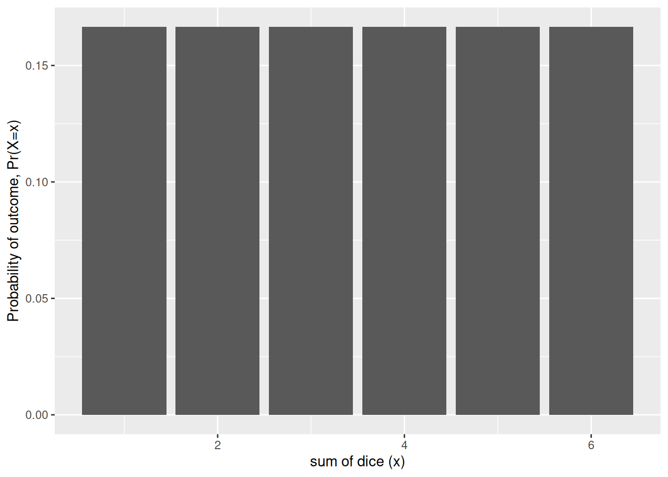
Example 1 (The sum of five dice) A single fair die roll has the discrete uniform distribution on \(\mathopen{}\left\{1, \ldots, 6\right\}\mathclose{}\), which is flat, not bell-shaped (Figure 1). Its mean is \(\mu = 3.5\), and its variance is \(\sigma^2= \sum_{x=1}^{6} (x - 3.5)^2 / 6 = 35/12\).
Show R code
dice_sum_pmf <-function(n_dice) { totals <-rowSums(expand.grid(rep(list(1:6), n_dice))) probs <-prop.table(table(totals))data.frame(total =as.numeric(names(probs)), p =as.vector(probs))}dice_plot <- ggplot2::ggplot(mapping = ggplot2::aes(x = total, y = p)) + ggplot2::xlab("sum of dice (x)") + ggplot2::ylab("Probability of outcome, Pr(X=x)") + ggplot2::expand_limits(y =0)dice_plot + ggplot2::geom_col(data =dice_sum_pmf(1))
Figure 1: Distribution of the outcome of one die
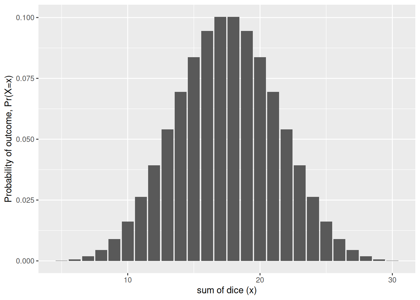
The sum of five independent rolls, \(S_5\), is already close to bell-shaped (Figure 2).
For example, the exact probability that five dice total at most 15 is \(\Pr(S_5 \le 15) = 0.3052\). The normal approximation that Theorem 1 suggests, with mean \(5 \cdot 3.5 = 17.5\) and variance \(5 \cdot 35/12 \approx 14.58\), evaluated at \(15.5\) to account for \(S_5\) taking only integer values, gives \(\Phi\mathopen{}\left((15.5 - 17.5)/\sqrt{14.58}\right)\mathclose{} \approx 0.3002\).
References
Billingsley, Patrick. 1995. Probability and Measure. 3rd ed. Wiley Series in Probability and Mathematical Statistics. Wiley.