Correlation and Simple Linear Regression

Published

Last modified: 2026-09-29 00:05:17 (PDT)

This page reviews two ways to relate two continuous variables: correlation coefficients, with tests of whether they differ from zero, and simple linear regression. It uses the $t$ reference distribution defined on the Statistical Inference page. This page is adapted from Vittinghoff et al. (2012), Chapter 3.

1 The HERS data

The examples on this page use the HERS data, which the Comparing Means page describes. The rmb R package includes the dataset; haven::as_factor() converts its Stata value labels to factors:

hers <- rmb::hers |> haven::as_factor()

2 Correlation

2.1 Testing the Pearson correlation

Definition 1 (Population correlation) The population correlation of two random variables $X$ and $Y$ with positive variances is

\[\rho \stackrel{\text{def}}{=}\frac{\operatorname{Cov}\mathopen{}\left(X, Y\right)\mathclose{}}{\sqrt{\operatorname{Var}\mathopen{}\left(X\right)\mathclose{} \operatorname{Var}\mathopen{}\left(Y\right)\mathclose{}}},\]

where $\operatorname{Cov}\mathopen{}\left(X, Y\right)\mathclose{}$ is their covariance.

The Pearson correlation coefficient $r$ of a sample is the corresponding sample statistic, and estimates $\rho$.

Definition 2 (Test of zero correlation) Let $r$ be the Pearson correlation coefficient of $n \ge 3$ pairs, with $\mathopen{}\left|r\right|\mathclose{} < 1$. The t-test of zero correlation of $H_0: \rho = 0$ against $H_1: \rho \neq 0$ (Definition 1) uses the statistic

\[t \stackrel{\text{def}}{=}\frac{r \sqrt{n - 2}}{\sqrt{1 - r^2}}.\]

Its p-value is $\Pr(\mathopen{}\left|T\right|\mathclose{} \ge \mathopen{}\left|t\right|\mathclose{})$, where $T$ has the $t_{n-2}$ distribution (t-distribution).

Theorem 1 (Null distribution of the correlation t statistic) Let the pairs $(X_1, Y_1), \ldots, (X_n, Y_n)$ be independent, and let each $Y_i$, given $X_1, \ldots, X_n$, be Gaussian with a mean and variance that do not depend on the $X$ values. Then the statistic $t$ of Definition 2 has the $t_{n-2}$ distribution (Hogg et al. 2019, sec. 9.6, pp. 472-473).

The conditions of Theorem 1 hold, for example, when the pairs are independent draws from a bivariate Gaussian distribution with $\rho = 0$.

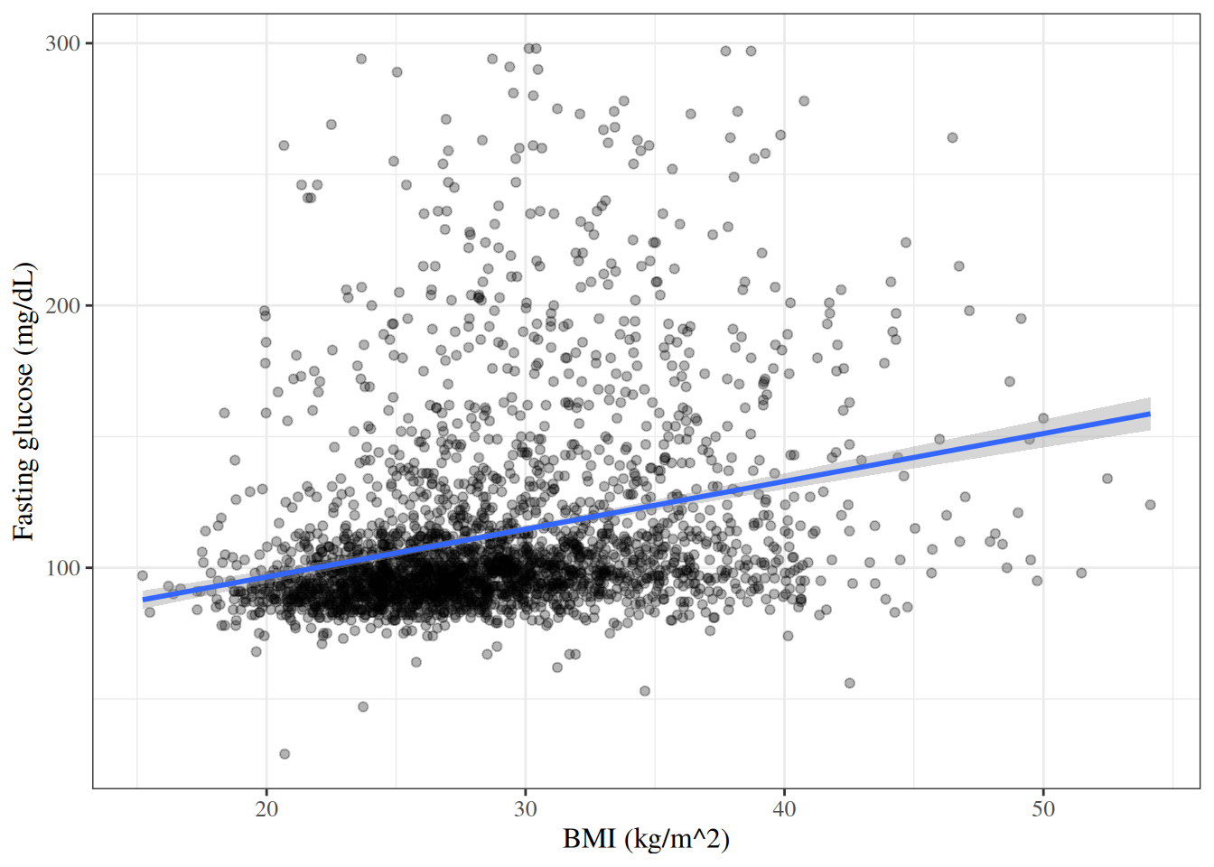
Example 1 (Correlation between BMI and fasting glucose in HERS) Figure 1 plots baseline fasting glucose against BMI.

Show R code

hers |>
  dplyr::filter(!is.na(BMI)) |>
  ggplot2::ggplot() +
  ggplot2::aes(x = BMI, y = glucose) +
  ggplot2::geom_point(alpha = 0.3) +
  ggplot2::geom_smooth(method = "lm", formula = y ~ x) +
  ggplot2::labs(
    x = "BMI (kg/m^2)",
    y = "Fasting glucose (mg/dL)"
  )

Figure 1: Baseline fasting glucose against BMI in HERS, with the least-squares line

The statistic of Definition 2, using the 2758 participants with a BMI measurement:

hers_bmi <- hers |> dplyr::filter(!is.na(BMI))
r <- cor(hers_bmi$BMI, hers_bmi$glucose)
n <- nrow(hers_bmi)
t_cor <- r * sqrt(n - 2) / sqrt(1 - r^2)
c(r = r, t = t_cor, p_value = 2 * pt(-abs(t_cor), df = n - 2))
#>           r           t     p_value 
#> 2.72664e-01 1.48779e+01 3.24201e-48

cor.test() reports the same values, and a confidence interval for $\rho$:

cor.test(hers$BMI, hers$glucose, method = "pearson")
#> 
#>  Pearson's product-moment correlation
#> 
#> data:  hers$BMI and hers$glucose
#> t = 14.88, df = 2756, p-value <2e-16
#> alternative hypothesis: true correlation is not equal to 0
#> 95 percent confidence interval:
#>  0.237760 0.306865
#> sample estimates:
#>      cor 
#> 0.272664

The correlation is positive but modest: glucose tends to be higher at higher BMI, with wide scatter around the line in Figure 1.

2.2 Spearman rank correlation

Definition 3 (Spearman rank correlation) Replace each $x_i$ by its rank among $x_1, \ldots, x_n$, and each $y_i$ by its rank among $y_1, \ldots, y_n$, giving tied values the average of the ranks they span. The Spearman rank correlation $r_S$ is the Pearson correlation coefficient of the ranks.

Because ranks depend only on the ordering of the values, $r_S$ measures how close the association is to monotone, whether or not it is linear, and a single extreme value moves $r_S$ less than it moves $r$.

Example 2 (Spearman correlation between BMI and fasting glucose in HERS) The Pearson correlation of the ranks (Definition 3), and cor.test()’s Spearman test (exact = FALSE, because tied values rule out the exact p-value):

hers_bmi <- hers |> dplyr::filter(!is.na(BMI))
cor(rank(hers_bmi$BMI), rank(hers_bmi$glucose))
#> [1] 0.333751
cor.test(hers_bmi$BMI, hers_bmi$glucose, method = "spearman", exact = FALSE)
#> 
#>  Spearman's rank correlation rho
#> 
#> data:  hers_bmi$BMI and hers_bmi$glucose
#> S = 2.33e+09, p-value <2e-16
#> alternative hypothesis: true rho is not equal to 0
#> sample estimates:
#>      rho 
#> 0.333751

$r_S$ is larger than the Pearson $r$ of Example 1: the association is closer to monotone than to linear.

3 Simple linear regression

3.1 Model specification

Definition 4 (Simple linear regression model) A simple linear regression model relates a continuous outcome $Y$ to a single predictor $X$:

\[Y_i = \beta_0 + \beta_1 x_i + \varepsilon_i, \qquad \varepsilon_1, \ldots, \varepsilon_n \ \sim_{\operatorname{iid}}\ \operatorname{N}\mathopen{}\left(0, \sigma^2\right)\mathclose{}.\]

$\beta_0$ is the intercept: the mean of $Y$ among observations with $X = 0$.
$\beta_1$ is the slope: the difference in the mean of $Y$ between two groups whose values of $X$ differ by one unit, $\beta_1 = \operatorname{E}\mathopen{}\left[Y \mid X = x + 1\right]\mathclose{} - \operatorname{E}\mathopen{}\left[Y \mid X = x\right]\mathclose{}$.
$\sigma^2$ is the variance of $Y$ around its mean at each value of $X$.

3.2 Ordinary least squares estimation

Definition 5 (Residual sum of squares) For data $(x_1, y_1), \ldots, (x_n, y_n)$, the residual sum of squares of a line with intercept $b_0$ and slope $b_1$ is

\[\text{RSS}(b_0, b_1) \stackrel{\text{def}}{=}\sum_{i=1}^n (y_i - b_0 - b_1 x_i)^2.\]

Example 3 (Residual sum of squares of a line through three points) For the points $(0, 1)$, $(1, 2)$, $(2, 2)$ and the line with $b_0 = 1$ and $b_1 = 0.5$, the vertical distances from the points to the line are $1 - 1 = 0$, $2 - 1.5 = 0.5$, and $2 - 2 = 0$, so $\text{RSS}(1, 0.5) = 0^2 + 0.5^2 + 0^2 = 0.25$.

Definition 6 (Ordinary least squares) The ordinary least squares (OLS) estimates $\hat\beta_0$ and $\hat\beta_1$ are the values of $b_0$ and $b_1$ that minimize the residual sum of squares $\text{RSS}(b_0, b_1)$.

Theorem 2 (Closed-form OLS estimates) Write

\[ \begin{aligned} S_{xx} &\stackrel{\text{def}}{=}\sum_{i=1}^n (x_i - \bar{x})^2, & S_{yy} &\stackrel{\text{def}}{=}\sum_{i=1}^n (y_i - \bar{y})^2, & S_{xy} &\stackrel{\text{def}}{=}\sum_{i=1}^n (x_i - \bar{x})(y_i - \bar{y}), \end{aligned} \]

and suppose $S_{xx} > 0$ (not all $x_i$ are equal). Then the OLS estimates (Definition 6) are unique, and

\[\hat\beta_1 = \frac{S_{xy}}{S_{xx}}, \qquad \hat\beta_0 = \bar{y} - \hat\beta_1 \bar{x}.\]

Proof

Proof. $\text{RSS}$ is a quadratic function of $(b_0, b_1)$, so we find where its partial derivatives are zero, then check that this point is the unique minimum.

The derivative with respect to $b_0$:

\[ \begin{aligned} \frac{\partial \text{RSS}}{\partial b_0} &= -2 \sum_{i=1}^n (y_i - b_0 - b_1 x_i) && \text{(chain rule, term by term)}\\ &= -2 \mathopen{}\left(n \bar{y} - n b_0 - b_1 n \bar{x}\right)\mathclose{} && \text{($\sum_i y_i = n\bar{y}$, $\sum_i x_i = n\bar{x}$)} \end{aligned} \]

Setting it to zero and dividing by $-2n$ gives $\bar{y} - b_0 - b_1 \bar{x} = 0$, so $b_0 = \bar{y} - b_1 \bar{x}$.

The derivative with respect to $b_1$, after substituting $b_0 = \bar{y} - b_1 \bar{x}$:

\[ \begin{aligned} \frac{\partial \text{RSS}}{\partial b_1} &= -2 \sum_{i=1}^n x_i (y_i - b_0 - b_1 x_i) && \text{(chain rule, term by term)}\\ &= -2 \sum_{i=1}^n x_i \mathopen{}\left((y_i - \bar{y}) - b_1 (x_i - \bar{x})\right)\mathclose{} && \text{(substitute $b_0$)}\\ &= -2 \sum_{i=1}^n (x_i - \bar{x}) \mathopen{}\left((y_i - \bar{y}) - b_1 (x_i - \bar{x})\right)\mathclose{} && \text{(subtract $\bar{x} \sum_i \mathopen{}\left((y_i - \bar{y}) - b_1 (x_i - \bar{x})\right)\mathclose{} = 0$)}\\ &= -2 \mathopen{}\left(S_{xy} - b_1 S_{xx}\right)\mathclose{} && \text{(definitions of $S_{xy}$ and $S_{xx}$)} \end{aligned} \]

The subtracted sum in the third step is zero because $\sum_i (y_i - \bar{y}) = 0$ and $\sum_i (x_i - \bar{x}) = 0$. Setting the derivative to zero gives $b_1 = S_{xy} / S_{xx}$.

This stationary point is the unique minimum. The matrix of second derivatives of $\text{RSS}$ is

\[ 2 \begin{pmatrix} n & n\bar{x} \\ n\bar{x} & \sum_i x_i^2 \end{pmatrix}, \]

whose top-left entry $2n$ is positive and whose determinant is $4\mathopen{}\left(n \sum_i x_i^2 - n^2 \bar{x}^2\right)\mathclose{} = 4 n S_{xx} > 0$. So the matrix is positive definite, $\text{RSS}$ is strictly convex, and its only stationary point is its global minimum.

Corollary 1 (OLS slope in terms of the correlation) If $S_{xx} > 0$ and $S_{yy} > 0$, then

\[\hat\beta_1 = r \, \frac{s_y}{s_x},\]

where $r$ is the Pearson correlation coefficient and $s_x$ and $s_y$ are the sample standard deviations of the $x_i$ and the $y_i$.

Proof

Proof. With the notation of Theorem 2, $r = S_{xy} / \sqrt{S_{xx} S_{yy}}$, $s_x = \sqrt{S_{xx} / (n-1)}$, and $s_y = \sqrt{S_{yy} / (n-1)}$. So:

\[ \begin{aligned} r \, \frac{s_y}{s_x} &= \frac{S_{xy}}{\sqrt{S_{xx} S_{yy}}} \cdot \frac{\sqrt{S_{yy} / (n-1)}}{\sqrt{S_{xx} / (n-1)}} && \text{(substitute $r$, $s_x$, $s_y$)}\\ &= \frac{S_{xy}}{\sqrt{S_{xx}} \sqrt{S_{yy}}} \cdot \frac{\sqrt{S_{yy}}}{\sqrt{S_{xx}}} && \text{(cancel the factors of $n - 1$)}\\ &= \frac{S_{xy}}{S_{xx}} && \text{(cancel $\sqrt{S_{yy}}$)}\\ &= \hat\beta_1 && \text{(closed-form OLS slope)} \end{aligned} \]

Video lecture

Hutchinson’s Linear Regression (pt1) (17 min) covers fitting a linear regression by least squares, framed as machine learning (Hutchinson, n.d.). The login for the video site is posted on Canvas.

3.3 Fitting a simple linear regression in R

Example 4 (Regression of fasting glucose on BMI in HERS) The OLS estimates from Theorem 2, and the slope from Corollary 1, for the participants with a BMI measurement:

hers_bmi <- hers |> dplyr::filter(!is.na(BMI))
x <- hers_bmi$BMI
y <- hers_bmi$glucose
b1 <- sum((x - mean(x)) * (y - mean(y))) / sum((x - mean(x))^2)
c(
  intercept = mean(y) - b1 * mean(x),
  slope = b1,
  slope_from_r = cor(x, y) * sd(y) / sd(x)
)
#>    intercept        slope slope_from_r 
#>     60.07405      1.82218      1.82218

lm() gives the same estimates:

slr_fit <- lm(glucose ~ BMI, data = hers)
summary(slr_fit)
#> 
#> Call:
#> lm(formula = glucose ~ BMI, data = hers)
#> 
#> Residuals:
#>    Min     1Q Median     3Q    Max 
#> -81.55 -18.98 -10.35   3.76 190.81 
#> 
#> Coefficients:
#>             Estimate Std. Error t value Pr(>|t|)    
#> (Intercept)   60.074      3.565    16.9   <2e-16 ***
#> BMI            1.822      0.122    14.9   <2e-16 ***
#> ---
#> Signif. codes:  0 '***' 0.001 '**' 0.01 '*' 0.05 '.' 0.1 ' ' 1
#> 
#> Residual standard error: 35.5 on 2756 degrees of freedom
#>   (5 observations deleted due to missingness)
#> Multiple R-squared:  0.0743, Adjusted R-squared:  0.074 
#> F-statistic:  221 on 1 and 2756 DF,  p-value: <2e-16

The estimated slope is $\hat\beta_1 = 1.82$ mg/dL per kg/m²: mean fasting glucose is about 1.8 mg/dL higher among participants whose BMI is 1 kg/m² higher. The t statistic for the slope equals the correlation test statistic of Example 1.

3.4 The coefficient of determination

Definition 7 (Total sum of squares) The total sum of squares of $y_1, \ldots, y_n$ is

\[\text{TSS} \stackrel{\text{def}}{=}\sum_{i=1}^n (y_i - \bar{y})^2.\]

Example 5 (Total sum of squares of three values) For $y = 1, 2, 2$, $\bar y = 5/3$, so

\[ \begin{aligned} \text{TSS} &= \mathopen{}\left(1 - \tfrac{5}{3}\right)\mathclose{}^2 + 2\mathopen{}\left(2 - \tfrac{5}{3}\right)\mathclose{}^2 && \text{(definition)}\\ &= \tfrac{4}{9} + \tfrac{2}{9} && \text{(square the deviations)}\\ &= \tfrac{2}{3} && \text{(arithmetic)} \end{aligned} \]

Definition 8 (Coefficient of determination) For a fitted regression with fitted values $\hat{y}_i$, the coefficient of determination is

\[R^2 \stackrel{\text{def}}{=}1 - \frac{\sum_{i=1}^n (y_i - \hat{y}_i)^2}{\sum_{i=1}^n (y_i - \bar{y})^2}.\]

The numerator is the residual sum of squares of the fit, and the denominator is the total sum of squares of the $y_i$.

$R^2$ is often described as the proportion of the variation in $Y$ explained by the regression on $X$.

Theorem 3 ($R^2$ of a simple linear regression) For the OLS fit of a simple linear regression, with $S_{xx} > 0$ and $S_{yy} > 0$, $R^2 = r^2$, where $r$ is the Pearson correlation coefficient of the $x_i$ and $y_i$. In particular, $0 \le R^2 \le 1$.

Proof

Proof. With the notation of Theorem 2, the fitted values are $\hat{y}_i = \hat\beta_0 + \hat\beta_1 x_i$, so each residual is

\[ \begin{aligned} y_i - \hat{y}_i &= y_i - (\bar{y} - \hat\beta_1 \bar{x}) - \hat\beta_1 x_i && \text{(substitute $\hat\beta_0$)}\\ &= (y_i - \bar{y}) - \hat\beta_1 (x_i - \bar{x}) && \text{(regroup)} \end{aligned} \]

Squaring and summing:

\[ \begin{aligned} \sum_{i=1}^n (y_i - \hat{y}_i)^2 &= \sum_{i=1}^n \mathopen{}\left((y_i - \bar{y})^2 - 2 \hat\beta_1 (x_i - \bar{x})(y_i - \bar{y}) + \hat\beta_1^2 (x_i - \bar{x})^2\right)\mathclose{} && \text{(expand the square)}\\ &= S_{yy} - 2 \hat\beta_1 S_{xy} + \hat\beta_1^2 S_{xx} && \text{(definitions of $S_{yy}$, $S_{xy}$, $S_{xx}$)}\\ &= S_{yy} - 2 \frac{S_{xy}^2}{S_{xx}} + \frac{S_{xy}^2}{S_{xx}} && \text{(substitute $\hat\beta_1 = S_{xy} / S_{xx}$)}\\ &= S_{yy} - \frac{S_{xy}^2}{S_{xx}} && \text{(combine like terms)} \end{aligned} \]

The total sum of squares is $S_{yy}$, so:

\[ \begin{aligned} R^2 &= 1 - \frac{S_{yy} - S_{xy}^2 / S_{xx}}{S_{yy}} && \text{(substitute into the definition of $R^2$)}\\ &= \frac{S_{xy}^2}{S_{xx} S_{yy}} && \text{(simplify)}\\ &= r^2 && \text{($r = S_{xy} / \sqrt{S_{xx} S_{yy}}$)} \end{aligned} \]

Since $-1 \le r \le 1$ (range of the correlation coefficient), $0 \le r^2 \le 1$.

Example 6 ($R^2$ for the regression of glucose on BMI in HERS) For the fit in Example 4, $R^2$ computed from Definition 8, the square of the Pearson correlation, and lm()’s value agree:

fit <- lm(glucose ~ BMI, data = hers)
y <- fit$model$glucose
c(
  r_squared = 1 - sum(residuals(fit)^2) / sum((y - mean(y))^2),
  cor_squared = cor(fit$model$BMI, y)^2,
  lm = summary(fit)$r.squared
)
#>   r_squared cor_squared          lm 
#>   0.0743455   0.0743455   0.0743455

BMI accounts for only about 7% of the variation in baseline fasting glucose.

3.5 Further reading

Linear Models Overview covers linear regression in depth, including inference for the coefficients and multiple predictors. Vittinghoff et al. (2012) cover linear regression in Chapter 4.

References

Hogg, Robert V., Elliot A. Tanis, and Dale L. Zimmerman. 2019. Probability and Statistical Inference. Tenth edition. Pearson.

Hutchinson, Brian. n.d. DATA 471/571 (Machine Learning) and CSCI 481/581 (Deep Learning) Video Lectures. Western Washington University. Accessed September 28, 2026. https://facultyweb.cs.wwu.edu/~hutchib2/video_lectures/data371/.

Vittinghoff, Eric, David V Glidden, Stephen C Shiboski, and Charles E McCulloch. 2012. Regression Methods in Biostatistics: Linear, Logistic, Survival, and Repeated Measures Models. 2nd ed. Springer. https://doi.org/10.1007/978-1-4614-1353-0.