birthwt <- read.csv("data/birthwt.csv")
fit <- lm(bwt ~ lwt, data = birthwt)
fitted_bwt <- fitted(fit)
residual <- birthwt$bwt - fitted_bwt
prediction_error <- fitted_bwt - birthwt$bwt
head(data.frame(
  bwt = birthwt$bwt,
  fitted = round(fitted_bwt, 1),
  residual = round(residual, 1),
  minus_prediction_error = round(-prediction_error, 1)
))Prediction
1 Predictions, fitted values, residuals, and prediction errors
DefDefinition 1 (Prediction (predicted value))
Definition 1 (Prediction (predicted value)) A prediction (or predicted value) \({\hat y\mathopen{}\left(x\right)\mathclose{}}\) of an outcome \(Y\) with covariate value \(X = x\) is a number computed from \(x\) and from data \((x_1, y_1), \ldots, (x_n, y_n)\) by a rule \(g\), and used as a guess of \(Y\):
\[{\hat y\mathopen{}\left(x\right)\mathclose{}} \stackrel{\text{def}}{=}g\mathopen{}\left(x; (x_1, y_1), \ldots, (x_n, y_n)\right)\mathclose{}.\]
ExmExample 1 (Predicting with an estimated conditional mean)
Example 1 (Predicting with an estimated conditional mean) Suppose a model specifies the conditional mean \({\mathbb{E}\mathopen{}\left[Y \mid X = x\right]\mathclose{}}\) as a function \(\mu(x; \mathord{\smash[b]{\underset{\raise.3ex\hbox{$\scriptstyle\sim$}}{\theta}}\vphantom{\theta}})\) of a parameter vector \(\mathord{\smash[b]{\underset{\raise.3ex\hbox{$\scriptstyle\sim$}}{\theta}}\vphantom{\theta}}\), and \(\hat{\mathord{\smash[b]{\underset{\raise.3ex\hbox{$\scriptstyle\sim$}}{\theta}}\vphantom{\theta}}}\) is an estimate of \(\mathord{\smash[b]{\underset{\raise.3ex\hbox{$\scriptstyle\sim$}}{\theta}}\vphantom{\theta}}\). The usual prediction (Definition 1) of \(Y\) at \(X = x\) is the estimated conditional mean:
\[{\hat y\mathopen{}\left(x\right)\mathclose{}} = \mu(x; \hat{\mathord{\smash[b]{\underset{\raise.3ex\hbox{$\scriptstyle\sim$}}{\theta}}\vphantom{\theta}}}).\]
RemarkRemark 1 (Why the estimated conditional mean is the usual prediction)
Remark 1 (Why the estimated conditional mean is the usual prediction). The prediction in Example 1 is chosen because the conditional mean is the best possible prediction under squared error loss. Among all functions \(h\) of the covariate, \({{\mathbb{E}\mathopen{}\left[Y \mid X\right]\mathclose{}}}\) has the smallest expected squared error \({\mathbb{E}\mathopen{}\left[{\mathopen{}\left(Y- {h\mathopen{}\left(X\right)\mathclose{}}\right)\mathclose{}}^{2}\right]\mathclose{}}\) (conditional mean minimizes squared-error risk). The conditional mean is unknown, so we estimate it from data and predict with the estimate.
The target depends on the loss. For absolute error loss, the best prediction is the conditional median instead, and other losses have other targets [1, p. 20].
DefDefinition 2 (Fitted value)
Definition 2 (Fitted value) The fitted value \(\hat y_i\) of observation \(i\) is the prediction at its own covariate value \(x_i\):
\[\hat y_i\stackrel{\text{def}}{=}{\hat y\mathopen{}\left(x_i\right)\mathclose{}}.\]
RemarkRemark 2 (Why the fitted value is the estimated conditional mean)
Remark 2 (Why the fitted value is the estimated conditional mean). The fitted value is the prediction at the observed covariate value \(x_i\), so for the prediction in Example 1 it is the estimated conditional mean at \(x_i\):
\[\hat y_i= \mu(x_i; \hat{\mathord{\smash[b]{\underset{\raise.3ex\hbox{$\scriptstyle\sim$}}{\theta}}\vphantom{\theta}}}).\]
It is chosen for the reason in Remark 1: the conditional mean is the best prediction under squared error loss.
DefDefinition 3 (Residual)
Definition 3 (Residual) The residual for observation \(i\) is its observed outcome minus its fitted value:
\[\hat{\varepsilon}_i\stackrel{\text{def}}{=}y_i- \hat y_i\]
Source: Wikipedia contributors [2].
DefDefinition 4 (Prediction error)
Definition 4 (Prediction error) The prediction error of a prediction \(\hat y\) (such as \({\hat y\mathopen{}\left(x\right)\mathclose{}}\) or a fitted value \(\hat y_i\)) of an observed outcome \(y\) is the prediction minus the outcome:
\[{\varepsilon_{\text{pred}}}\stackrel{\text{def}}{=}\hat y- y.\]
ExrExercise 1 (Prediction error and residual)
Exercise 1 (Prediction error and residual) For an observation \(i\), write its prediction error \({\varepsilon_{\text{pred}}}_i\) in terms of its residual \(\hat{\varepsilon}_i\).
LemTheorem 1 (Prediction error is the negative of the residual)
Theorem 1 (Prediction error is the negative of the residual) For an observation \(i\), the prediction error of its fitted value is the negative of its residual:
\[{\varepsilon_{\text{pred}}}_i= -\hat{\varepsilon}_i.\]
ProofProof
Proof. This is the solution to Exercise 1.
CorCorollary 1 (The residual is the negative of the prediction error)
Corollary 1 (The residual is the negative of the prediction error) For an observation \(i\), its residual is the negative of the prediction error of its fitted value:
\[\hat{\varepsilon}_i= -{\varepsilon_{\text{pred}}}_i.\]
ProofProof
Proof. Multiply both sides of Theorem 1 by \(-1\).
ExmExample 2 (Residuals and prediction errors for birth weights)
Example 2 (Residuals and prediction errors for birth weights) The birthwt data record the birth weight (grams) of 189 babies and their mothers’ weight at the last menstrual period (pounds), from a study at Baystate Medical Center in Springfield, Massachusetts [3]. They ship with the R package MASS (MASS::birthwt), and this site has a copy at data/birthwt.csv.
The code below fits a line predicting birth weight from mother’s weight, then compares each residual with the negative of its prediction error.
import numpy as np
import pandas as pd

birthwt = pd.read_csv("data/birthwt.csv")
X = np.column_stack([np.ones(len(birthwt)), birthwt["lwt"]])
y = birthwt["bwt"].to_numpy(dtype=float)
coef = np.linalg.lstsq(X, y, rcond=None)[0]
fitted_bwt = X @ coef
residual = y - fitted_bwt
prediction_error = fitted_bwt - y
print(pd.DataFrame({
    "bwt": y,
    "fitted": fitted_bwt.round(1),
    "residual": residual.round(1),
    "minus_prediction_error": (-prediction_error).round(1),
}).head())
#>       bwt  fitted  residual  minus_prediction_error
#> 0  2523.0  3175.7    -652.7                  -652.7
#> 1  2551.0  3056.1    -505.1                  -505.1
#> 2  2557.0  2834.7    -277.7                  -277.7
#> 3  2594.0  2848.0    -254.0                  -254.0
#> 4  2600.0  2843.5    -243.5                  -243.5
print(np.max(np.abs(residual - (-prediction_error))))
#> 0.0
The last two columns agree in every row, and the largest difference between them over all 189 babies is 0, as Corollary 1 says.
RemarkRemark 3 (Prediction errors and residuals)
Remark 3 (Prediction errors and residuals). The prediction in Definition 4 can be a fitted value, for an observation used to fit the model, or a prediction for an observation that was not used to fit the model. Prediction error is oriented the same way as estimation error: estimate minus true value.
\[ \begin{aligned} {\varepsilon_{\text{pred}}}&= \hat y- y && \text{(prediction error)}\\ {\varepsilon\mathopen{}\left(\hat{\theta}\right)\mathclose{}} &= \hat{\theta}- \theta && \text{(estimation error)} \end{aligned} \]
For a fitted value, the prediction error is the negative of the residual (Theorem 1), so the two differ only in orientation.
2 Sample mean squared error of predictions
DefDefinition 5 (Mean squared error of predictions)
Definition 5 (Mean squared error of predictions) The sample mean squared error (sMSE) of predictions, also called their mean squared error, \(\hat y_1, \ldots, \hat y_n\) of observed outcomes \(y_1, \ldots, y_n\) is the mean of their squared prediction errors:
\[{\operatorname{sMSE}\mathopen{}\left(\hat y\right)\mathclose{}} \stackrel{\text{def}}{=}\frac{1}{n}\sum_{i=1}^n{\varepsilon_{\text{pred}}}_i^2.\]
Source: Wikipedia contributors [4].
RemarkRemark 4 (Prediction sMSE, estimator pMSE and RSS)
Remark 4 (Prediction sMSE, estimator pMSE and RSS). Definition 5 averages squared errors over observations, where the pMSE of an estimator takes an expectation over repeated samples. On the data used to fit the model, the sMSE of the fitted values is the residual sum of squares divided by \(n\) (sMSE and RSS):
\[{\operatorname{sMSE}\mathopen{}\left(\hat y\right)\mathclose{}} = \frac{1}{n} \text{RSS}(\hat{\mathord{\smash[b]{\underset{\raise.3ex\hbox{$\scriptstyle\sim$}}{\theta}}\vphantom{\theta}}}), \qquad \text{RSS}(\hat{\mathord{\smash[b]{\underset{\raise.3ex\hbox{$\scriptstyle\sim$}}{\theta}}\vphantom{\theta}}}) = n \, {\operatorname{sMSE}\mathopen{}\left(\hat y\right)\mathclose{}}.\]
ExmExample 3 (Fitted values, residuals, and prediction errors for three points)
Example 3 (Fitted values, residuals, and prediction errors for three points) Take the points \((0, 1)\), \((1, 2)\), \((2, 2)\) and the line with \(\beta_{0}= 1\) and \(\beta_{x} = 0.5\) from the residual sum of squares example, and treat the line as the fitted model.
| \(x_i\) | \(y_i\) | \(\hat y_i= 1 + 0.5 x_i\) | \(\hat{\varepsilon}_i= y_i- \hat y_i\) | \({\varepsilon_{\text{pred}}}_i= \hat y_i- y_i\) |
|---|---|---|---|---|
| 0 | 1 | 1 | 0 | 0 |
| 1 | 2 | 1.5 | 0.5 | \(-0.5\) |
| 2 | 2 | 2 | 0 | 0 |
Figure 1 shows the observed outcomes, the fitted values on the line, and the residual of the second point.
Show R code
fre_points <- tibble::tibble(x = c(0, 1, 2), y = c(1, 2, 2)) |>
  dplyr::mutate(fitted = 1 + 0.5 * x)

ggplot2::ggplot(fre_points, ggplot2::aes(x = x)) +
  ggplot2::geom_abline(intercept = 1, slope = 0.5) +
  ggplot2::geom_segment(
    ggplot2::aes(y = fitted, xend = x, yend = y),
    linetype = "dashed",
    color = "firebrick"
  ) +
  ggplot2::geom_point(ggplot2::aes(y = fitted), shape = 1, size = 3) +
  ggplot2::geom_point(ggplot2::aes(y = y), size = 3) +
  ggplot2::annotate(
    "text",
    x = 1.1, y = 1.75, hjust = 0,
    label = "r[2] == 0.5", parse = TRUE
  ) +
  ggplot2::labs(y = "Response, y")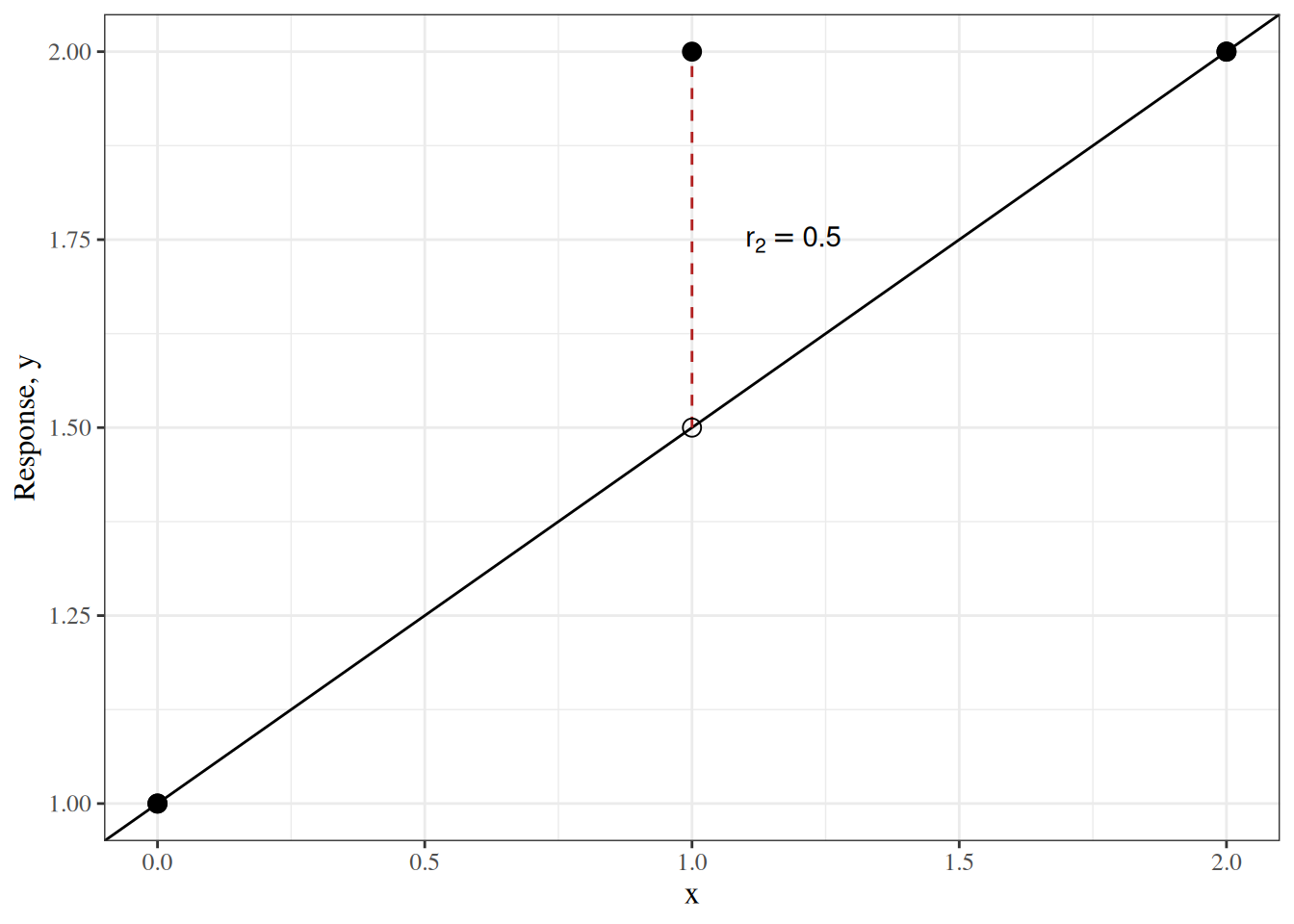
The sMSE of these predictions is
\[ \begin{aligned} {\operatorname{sMSE}\mathopen{}\left(\hat y\right)\mathclose{}} &= \frac{0^2 + (-0.5)^2 + 0^2}{3}\\ &= \frac{0.25}{3}\\ &\approx 0.083, \end{aligned} \]
the residual sum of squares, \(0.25\), divided by \(n = 3\).
3 Estimation versus prediction
RemarkRemark 5 (Estimation versus prediction)
Remark 5 (Estimation versus prediction). Estimation and prediction both measure error as a signed difference, and both summarize it with a mean squared error (a pMSE for an estimator, an sMSE for predictions), but they aim at different targets:
- Target. An estimate aims at a fixed, unknown estimand. A prediction aims at an outcome \(y\), which is a random quantity even when the model is known exactly.
- Error. The estimation error is the estimate minus the estimand. The prediction error is the prediction minus the outcome.
- Mean squared error. The pMSE of an estimator is an expectation over repeated samples. The sMSE of predictions is an average over observations.
- What cannot be removed. The estimation error of a consistent estimator shrinks toward zero as the sample grows. A prediction’s expected squared error, given the same covariates, cannot fall below the residual variance, the variance of the outcome around its conditional mean.
Validating Predictions estimates the prediction error on new observations.
References
[1]
T. Hastie, R. Tibshirani, and J. Friedman, The elements of statistical learning: Data mining, inference, and prediction, 2nd ed. Springer, 2009. doi: 10.1007/978-0-387-84858-7.
[2]
Wikipedia contributors, “Errors and residuals — Wikipedia, the free encyclopedia.” 2026. Available: https://en.wikipedia.org/wiki/Errors_and_residuals
[3]
D. W. Hosmer and S. Lemeshow, Applied logistic regression. New York: Wiley, 1989.
[4]
Wikipedia contributors, “Mean squared prediction error — Wikipedia, the free encyclopedia.” 2026. Available: https://en.wikipedia.org/wiki/Mean_squared_prediction_error