Published

Last modified: 2026-11-19

Show code
# The Python chunks on this page import matplotlib, pandas and scikit-learn;
# reticulate provisions them.
py_packages <- c("matplotlib", "numpy", "pandas", "scikit-learn")
library(reticulate) # nolint: undesirable_function_linter
library(tidymodels) # nolint: undesirable_function_linter
py_require(py_packages)
1 The book’s Chapter 8 lab

This page holds the code lab for the Ensemble Methods chapter.

To work the lab without the solutions, download a stub with only the exercises:

Each solution shows the code in Python and in R.

Section 8.3 of the book [1] is the source of these exercises. The Python code uses scikit-learn [2], and the R code uses the rpart, ranger and xgboost engines of tidymodels.

2 Exploring the Carseats data

DatasetDataset 1: The car seat sales (Carseats) data
Dataset 1: The car seat sales (Carseats) data

Simulated sales of child car seats at 400 stores make up the Carseats data [1, Sec. 8.3.1]. The data are in data/carseats.csv, one row per store. The columns this course uses are:

  • Sales: the unit sales, in thousands, at the store.
  • Price: the price the company charges for a car seat at the store.
  • ShelveLoc: the quality of the shelving location, Bad, Medium or Good.
  • The other columns: the local population, income and advertising budget, among other store characteristics.
ExrExercise 1 (Lab: the scale of sales)

Exercise 1 (Lab: the scale of sales) Use the Carseats data. What are the sample mean and sample standard deviation of Sales?

TipHint

Read the file into a table, then apply a summary function to one column.

Solution 1.

import pandas as pd

cs_eda_py = pd.read_csv("data/carseats.csv")
cs_eda_py_mean = float(cs_eda_py["Sales"].mean())
cs_eda_py_sd = float(cs_eda_py["Sales"].std())
round(cs_eda_py_mean, 2), round(cs_eda_py_sd, 2)
(7.5, 2.82)
cs_eda_r <- readr::read_csv("data/carseats.csv", show_col_types = FALSE)
cs_eda_r_mean <- mean(cs_eda_r$Sales)
cs_eda_r_sd <- sd(cs_eda_r$Sales)
c(mean = cs_eda_r_mean, sd = cs_eda_r_sd)
    mean       sd 
7.496325 2.824115 

Across the 400 stores, Sales has a mean of 7.5 thousand units and a standard deviation of 2.82 thousand. The lab’s next exercises split the stores at \(8\) thousand units, which is slightly above this mean.

ExrExercise 2 (Lab: stores by shelving location)

Exercise 2 (Lab: stores by shelving location) Use the Carseats data. How many stores have each value of ShelveLoc?

TipHint

Count the rows with each value of a column using a pandas method in Python, or count() in R.

Solution 2. This solution continues Solution 1.

cs_eda_py["ShelveLoc"].value_counts()
ShelveLoc
Medium    219
Bad        96
Good       85
Name: count, dtype: int64
cs_eda_r_shelve <- count(cs_eda_r, ShelveLoc)
cs_eda_r_shelve
Show code
cs_eda_r_medium <- filter(cs_eda_r_shelve, ShelveLoc == "Medium")

Medium is the most common location, with 219 of the 400 stores. ShelveLoc has three values rather than numbers, so a tree can split on it, but a straight-line formula would first need it recoded.

ExrExercise 3 (Lab: a histogram of sales)

Exercise 3 (Lab: a histogram of sales) Use the Carseats data. Draw a histogram of Sales.

TipHint

Draw a histogram of one column, as in the histogram of the year of each car in the primer.

Solution 3. This solution continues Solution 2.

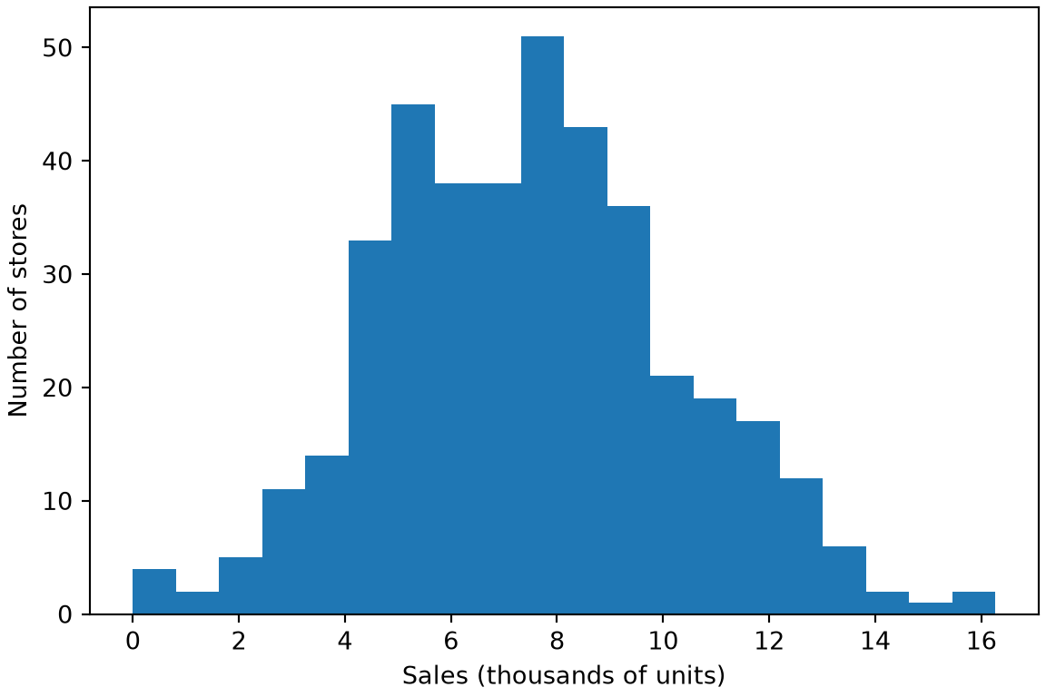
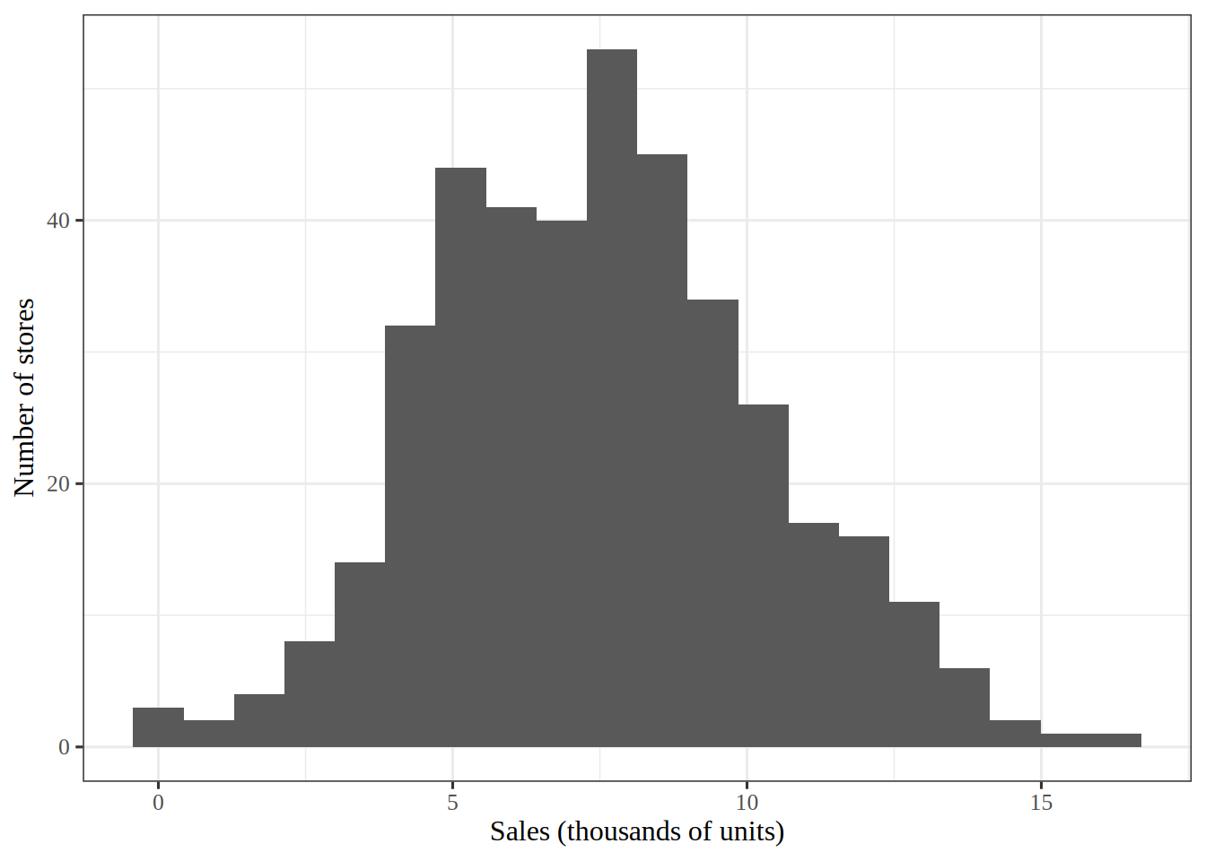
Figure 1: Bars counting the stores at each level of car seat sales, in thousands of units.
import matplotlib.pyplot as plt

fig, ax = plt.subplots(figsize=(6, 4), layout="constrained")
ax.hist(cs_eda_py["Sales"], bins=20);
ax.set_xlabel("Sales (thousands of units)");
ax.set_ylabel("Number of stores");
plt.show()

Histogram of car seat sales in thousands of units at 400 stores, with a broad hump around 5 to 9 and a thin right tail.

library(ggplot2) # nolint: undesirable_function_linter

sales_histogram <- cs_eda_r |>
  ggplot() +
  aes(Sales) +
  geom_histogram(bins = 20) +
  labs(x = "Sales (thousands of units)", y = "Number of stores")
sales_histogram

Histogram of car seat sales in thousands of units at 400 stores, with a broad hump around 5 to 9 and a thin right tail.

Show code
cs_eda_r_per_bin <- nrow(cs_eda_r) / 20

Figure 1 shows a broad hump of sales between 5 and 9 thousand units, with a thin right tail.

I chose 20 bins, which is 20 stores per bar on average. Far fewer bins would hide the shape inside a few wide bars, and far more would leave most bars with only a few stores, so the outline would look ragged. That is why 20 is a compromise between the two.

ExrExercise 4 (Lab: sales against price)

Exercise 4 (Lab: sales against price) Use the Carseats data. Draw a scatterplot of Sales against Price.

TipHint

Draw a scatterplot of one column against another, as in the plot of acceleration against horsepower in the primer.

Solution 4. This solution continues Solution 3.

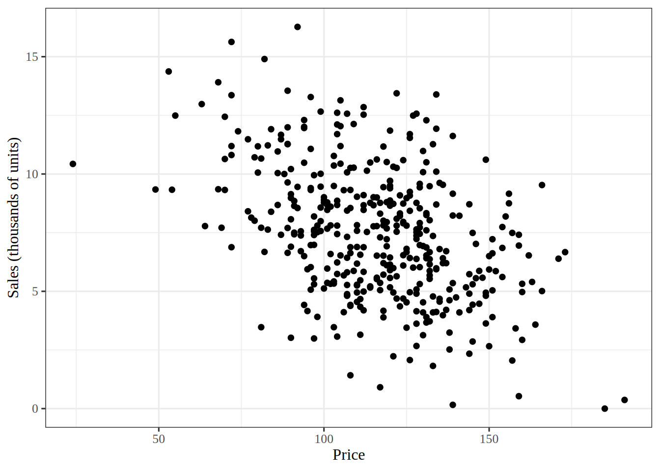
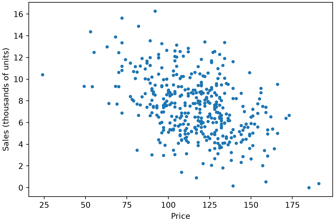
Figure 2: Car seat sales, in thousands of units, against price, with one dot per store.
fig, ax = plt.subplots(figsize=(6, 4), layout="constrained")
ax.scatter(cs_eda_py["Price"], cs_eda_py["Sales"], s=10);
ax.set_xlabel("Price");
ax.set_ylabel("Sales (thousands of units)");
plt.show()

Scatterplot of car seat sales in thousands of units against price. The points drift downward from left to right inside a wide cloud with a lot of scatter.

sales_price_plot <- cs_eda_r |>
  ggplot() +
  aes(Price, Sales) +
  geom_point() +
  labs(x = "Price", y = "Sales (thousands of units)")
sales_price_plot

Scatterplot of car seat sales in thousands of units against price. The points drift downward from left to right inside a wide cloud with a lot of scatter.

In Figure 2, stores with a higher price tend to sell fewer car seats, but the cloud is wide, so price alone leaves most of the variation in Sales unexplained. Other variables, such as ShelveLoc, have to explain the rest.

3 Classification trees

ExrExercise 5 (Lab: define a high-sales indicator)

Exercise 5 (Lab: define a high-sales indicator) Read the Carseats data from data/carseats.csv, which are simulated sales of child car seats at \(400\) stores [1]. Add a variable High that is "Yes" for a store whose Sales (in thousands of units) exceed \(8\) and "No" otherwise.

TipHint

The data frame functions read the file, and .assign adds a column computed from another one. In R, mutate() does the same.

Solution 5.

import pandas as pd

carseats_py = pd.read_csv("data/carseats.csv")
carseats_py["High"] = carseats_py["Sales"].gt(8).map({True: "Yes", False: "No"})
carseats_py["High"].value_counts()
High
No     236
Yes    164
Name: count, dtype: int64
carseats <- readr::read_csv("data/carseats.csv", show_col_types = FALSE) |>
  mutate(High = factor(if_else(Sales > 8, "Yes", "No")))
count(carseats, High)

The data have 400 stores, and 41% of them have Sales above \(8\).

ExrExercise 6 (Lab: split the Carseats data)

Exercise 6 (Lab: split the Carseats data) Split the Carseats stores from Exercise 5 at random into a training set and a test set of equal size, using every variable except Sales as a feature of High.

TipHint

The random number functions draw row positions without repeats, and a selection by position keeps those rows.

Solution 6.

from sklearn.model_selection import train_test_split

x_py = pd.get_dummies(
    carseats_py.drop(columns=["Sales", "High"]), drop_first=True
)
split_py = train_test_split(
    x_py, carseats_py["High"], test_size=0.5, random_state=0
)
x_train_py, x_test_py, high_train_py, high_test_py = split_py
(len(high_train_py), len(high_test_py))
(200, 200)
set.seed(571)
carseats_high <- select(carseats, -Sales)
split_carseats <- initial_split(carseats_high, prop = 1 / 2)
train_carseats <- training(split_carseats)
test_carseats <- testing(split_carseats)
n_train <- nrow(train_carseats)
n_test <- nrow(test_carseats)
c(n_train, n_test)
[1] 200 200

The training set and the test set hold 200 and 200 stores in the R run, and 200 and 200 in the Python run. The two runs use different random splits.

ExrExercise 7 (Lab: fit a classification tree)

Exercise 7 (Lab: fit a classification tree) Fit a classification tree of High on the other variables in the training set from Exercise 6, with at most \(5\) levels of splits.

TipHint

Every estimator in scikit-learn is fit with .fit on a matrix of features and a vector of outcomes, so a column of text must first be recoded to indicator columns. In R, the decision_tree() specification of tidymodels is fit with fit().

Solution 7.

from sklearn.tree import DecisionTreeClassifier

tree_py = DecisionTreeClassifier(max_depth=5, random_state=0)
tree_py.fit(x_train_py, high_train_py)
DecisionTreeClassifier(max_depth=5, random_state=0)
In a Jupyter environment, please rerun this cell to show the HTML representation or trust the notebook.
On GitHub, the HTML representation is unable to render, please try loading this page with nbviewer.org.
tree_py.get_n_leaves()
np.int64(22)
tree_spec <- decision_tree(tree_depth = 5) |>
  set_engine("rpart") |>
  set_mode("classification")
tree_carseats <- fit(tree_spec, High ~ ., data = train_carseats)
tree_carseats
parsnip model object

n= 200 

node), split, n, loss, yval, (yprob)
      * denotes terminal node

 1) root 200 76 No (0.62000000 0.38000000)  
   2) ShelveLoc=Bad,Medium 160 44 No (0.72500000 0.27500000)  
     4) Advertising< 13.5 133 28 No (0.78947368 0.21052632)  
       8) Price>=105 90 11 No (0.87777778 0.12222222)  
        16) CompPrice< 147.5 80  5 No (0.93750000 0.06250000) *
        17) CompPrice>=147.5 10  4 Yes (0.40000000 0.60000000) *
       9) Price< 105 43 17 No (0.60465116 0.39534884)  
        18) Age>=61.5 18  1 No (0.94444444 0.05555556) *
        19) Age< 61.5 25  9 Yes (0.36000000 0.64000000)  
          38) CompPrice< 112.5 9  3 No (0.66666667 0.33333333) *
          39) CompPrice>=112.5 16  3 Yes (0.18750000 0.81250000) *
     5) Advertising>=13.5 27 11 Yes (0.40740741 0.59259259)  
      10) Age>=54.5 14  4 No (0.71428571 0.28571429) *
      11) Age< 54.5 13  1 Yes (0.07692308 0.92307692) *
   3) ShelveLoc=Good 40  8 Yes (0.20000000 0.80000000)  
     6) Price>=135 7  2 No (0.71428571 0.28571429) *
     7) Price< 135 33  3 Yes (0.09090909 0.90909091) *
ExrExercise 8 (Lab: test the classification tree)

Exercise 8 (Lab: test the classification tree) Report the error rate of the tree from Exercise 7 on the test set.

TipHint

The .predict method returns predicted classes, and the error rate is the share that differ from the actual ones. In R, predict() on a tidymodels workflow plays the same role as .predict.

Solution 8.

error_tree_py = (tree_py.predict(x_test_py) != high_test_py).mean()
error_tree_py
np.float64(0.345)
pred_carseats <- predict(tree_carseats, new_data = test_carseats)
error_tree_r <- mean(pred_carseats$.pred_class != test_carseats$High)
error_tree_r
[1] 0.255

The test error rate is 0.255 in the R run and 0.345 in the Python run. The two runs use different random splits, so the two rates differ by more than the choice of language.

4 Regression trees

ExrExercise 9 (Lab: split the Boston data)

Exercise 9 (Lab: split the Boston data) Download the Boston data from data/boston.csv, which has \(506\) Boston neighborhoods from the 1970 census [3]. Its response medv is the median home value, in thousands of dollars. Split the neighborhoods at random into a training set and a test set of equal size.

TipHint

The data frame functions read the file, and the random number functions draw the row positions of the training set.

Solution 9.

import pandas as pd
from sklearn.model_selection import train_test_split

boston_py = pd.read_csv("data/boston.csv")
x_boston_py = boston_py.drop(columns="medv")
split_boston_py = train_test_split(
    x_boston_py, boston_py["medv"], test_size=0.5, random_state=0
)
x_train_b, x_test_b, y_train_b, y_test_b = split_boston_py
(len(y_train_b), len(y_test_b))
(253, 253)
boston <- readr::read_csv("data/boston.csv", show_col_types = FALSE)
set.seed(571)
split_boston <- initial_split(boston, prop = 1 / 2)
train_boston <- training(split_boston)
test_boston <- testing(split_boston)
n_train_b <- nrow(train_boston)
n_test_b <- nrow(test_boston)
c(n_train_b, n_test_b)
[1] 253 253

The training set and the test set hold 253 and 253 neighborhoods in the R run, and 253 and 253 in the Python run. The two runs use different random splits.

ExrExercise 10 (Lab: fit a regression tree)

Exercise 10 (Lab: fit a regression tree) Fit a regression tree of medv on the other variables in the training set from Exercise 9, with at most \(4\) levels of splits.

TipHint

The regression tree estimator is fit with .fit, and one of its settings limits the number of levels of splits. In R, the decision_tree() specification of tidymodels is fit with fit().

Solution 10.

from sklearn.tree import DecisionTreeRegressor

reg_py = DecisionTreeRegressor(max_depth=4, random_state=0)
reg_py.fit(x_train_b, y_train_b)
DecisionTreeRegressor(max_depth=4, random_state=0)
In a Jupyter environment, please rerun this cell to show the HTML representation or trust the notebook.
On GitHub, the HTML representation is unable to render, please try loading this page with nbviewer.org.
reg_py.get_n_leaves()
np.int64(15)
reg_spec <- decision_tree(tree_depth = 4) |>
  set_engine("rpart") |>
  set_mode("regression")
reg_r <- fit(reg_spec, medv ~ ., data = train_boston)
reg_r
parsnip model object

n= 253 

node), split, n, deviance, yval
      * denotes terminal node

 1) root 253 21489.4600 23.12253  
   2) rm< 6.9715 212  7070.3550 20.15849  
     4) lstat>=15 70  1037.9830 14.66286  
       8) crim>=5.76921 32   258.6722 11.76562 *
       9) crim< 5.76921 38   284.5097 17.10263 *
     5) lstat< 15 142  2876.0510 22.86761  
      10) rm< 6.491 107   744.3888 21.18037 *
      11) rm>=6.491 35   895.8469 28.02571  
        22) lstat>=5.155 24   205.5733 26.28333 *
        23) lstat< 5.155 11   458.4418 31.82727 *
   3) rm>=6.9715 41  2925.9220 38.44878  
     6) lstat>=4.505 25   848.9864 33.08800  
      12) tax>=267 13   190.0200 29.60000 *
      13) tax< 267 12   329.4667 36.86667 *
     7) lstat< 4.505 16   235.9100 46.82500 *
ExrExercise 11 (Lab: test the regression tree)

Exercise 11 (Lab: test the regression tree) Report the mean squared error of the tree from Exercise 10 on the test set.

TipHint

The .predict method and the error function of scikit-learn give the mean squared error on the held-out rows. In R, predict() on a tidymodels workflow plays the same role as .predict.

Solution 11.

mse_tree_py = ((reg_py.predict(x_test_b) - y_test_b) ** 2).mean()
mse_tree_py
np.float64(23.585130011852332)
pred_boston <- predict(reg_r, new_data = test_boston)
mse_tree_r <- mean((pred_boston$.pred - test_boston$medv)^2)
mse_tree_r
[1] 31.72017

The test mean squared error is 31.7 in the R run and 23.6 in the Python run, in squared thousands of dollars. The two runs use different random splits, so the two errors differ by more than the choice of language.

5 Random forests

ExrExercise 12 (Lab: fit a random forest)

Exercise 12 (Lab: fit a random forest) Fit a random forest of \(500\) regression trees of medv on the other variables in the training set from Exercise 9. At each split, let the forest choose among \(6\) of the \(12\) predictors, picked at random.

TipHint

Every estimator in scikit-learn is fit with .fit, and a random forest has settings for the number of trees and for the number of predictors tried at each split. In R, the rand_forest() specification of tidymodels has the same settings and is fit with fit().

Solution 12.

from sklearn.ensemble import RandomForestRegressor

forest_py = RandomForestRegressor(
    n_estimators=500, max_features=6, random_state=0
)
forest_py.fit(x_train_b, y_train_b)
RandomForestRegressor(max_features=6, n_estimators=500, random_state=0)
In a Jupyter environment, please rerun this cell to show the HTML representation or trust the notebook.
On GitHub, the HTML representation is unable to render, please try loading this page with nbviewer.org.
len(forest_py.estimators_)
500
forest_spec <- rand_forest(trees = 500, mtry = 6) |>
  set_engine("ranger") |>
  set_mode("regression")
forest_r <- fit(forest_spec, medv ~ ., data = train_boston)
forest_r
parsnip model object

Ranger result

Call:
 ranger::ranger(x = maybe_data_frame(x), y = y, mtry = min_cols(~6,      x), num.trees = 500, num.threads = 1, verbose = FALSE, seed = sample.int(10^5,      1)) 

Type:                             Regression 
Number of trees:                  500 
Sample size:                      253 
Number of independent variables:  12 
Mtry:                             6 
Target node size:                 5 
Variable importance mode:         none 
Splitrule:                        variance 
OOB prediction error (MSE):       12.96487 
R squared (OOB):                  0.8479652 

The Python code fits the forest with scikit-learn’s RandomForestRegressor, and the R code fits it with the ranger engine of tidymodels. Both average the predictions of the \(500\) trees.

ExrExercise 13 (Lab: test the random forest)

Exercise 13 (Lab: test the random forest) Report the mean squared error of the forest from Exercise 12 on the test set.

TipHint

The .predict method and the error function of scikit-learn give the mean squared error on the held-out rows. In R, predict() on a tidymodels workflow plays the same role as .predict.

Solution 13.

mse_forest_py = ((forest_py.predict(x_test_b) - y_test_b) ** 2).mean()
mse_forest_py
np.float64(16.147031375810304)
pred_forest <- predict(forest_r, new_data = test_boston)
mse_forest_r <- mean((pred_forest$.pred - test_boston$medv)^2)
mse_forest_r
[1] 16.42938

The test mean squared error is 16.4 in the R run and 16.1 in the Python run, compared with 31.7 and 23.6 for the single regression tree. The forest’s test error is lower than the single tree’s in the R run and lower in the Python run. The two runs use different random splits, so compare the R and Python values only within each run.

6 Boosting

ExrExercise 14 (Lab: fit a boosted regression)

Exercise 14 (Lab: fit a boosted regression) Fit a boosted ensemble of \(5000\) regression trees of medv on the other variables in the training set from Exercise 9. Give each tree at most \(4\) levels of splits, and use the learning rate \(0.2\).

TipHint

Every estimator in scikit-learn is fit with .fit; a boosted ensemble has settings for the number of trees, the number of levels of each tree and the learning rate. In R, the boost_tree() specification of tidymodels has the same settings and is fit with fit().

Solution 14.

from sklearn.ensemble import GradientBoostingRegressor

boost_py = GradientBoostingRegressor(
    n_estimators=5000, max_depth=4, learning_rate=0.2, random_state=0
)
boost_py.fit(x_train_b, y_train_b)
GradientBoostingRegressor(learning_rate=0.2, max_depth=4, n_estimators=5000,
                          random_state=0)
In a Jupyter environment, please rerun this cell to show the HTML representation or trust the notebook.
On GitHub, the HTML representation is unable to render, please try loading this page with nbviewer.org.
boost_py.n_estimators_
5000
boost_spec <- boost_tree(trees = 5000, tree_depth = 4, learn_rate = 0.2) |>
  set_engine("xgboost") |>
  set_mode("regression")
boost_r <- fit(boost_spec, medv ~ ., data = train_boston)
boost_r
parsnip model object

##### xgb.Booster
call:
  xgboost::xgb.train(params = list(eta = 0.2, max_depth = 4, gamma = 0, 
    colsample_bytree = 1, colsample_bynode = 1, min_child_weight = 1, 
    subsample = 1, nthread = 1, objective = "reg:squarederror"), 
    data = x$data, nrounds = 5000, evals = x$watchlist, verbose = 0)
# of features: 12 
# of rounds:  5000 
callbacks:
   evaluation_log 
evaluation_log:
  iter training_rmse
 <num>         <num>
     1    7.67655235
     2    6.45071980
   ---           ---
  4999    0.00166229
  5000    0.00166229

The Python code fits the ensemble with scikit-learn’s GradientBoostingRegressor, and the R code fits it with the xgboost engine of tidymodels. Both add the \(5000\) trees one at a time, each fitted to the residuals of the trees before it.

ExrExercise 15 (Lab: test the boosted regression)

Exercise 15 (Lab: test the boosted regression) Report the mean squared error of the boosted ensemble from Exercise 14 on the test set.

TipHint

The .predict method and the error function of scikit-learn give the mean squared error on the held-out rows. In R, predict() on a tidymodels workflow plays the same role as .predict.

Solution 15.

mse_boost_py = ((boost_py.predict(x_test_b) - y_test_b) ** 2).mean()
mse_boost_py
np.float64(16.61467329151459)
pred_boost <- predict(boost_r, new_data = test_boston)
mse_boost_r <- mean((pred_boost$.pred - test_boston$medv)^2)
mse_boost_r
[1] 17.99549

The test mean squared error is 18 in the R run and 16.6 in the Python run, compared with 16.4 and 16.1 for the random forest. The two runs use different random splits, so compare the R and Python values only within each run.

References

[1]
G. James, D. Witten, T. Hastie, R. Tibshirani, and J. Taylor, An introduction to statistical learning: With applications in Python. Springer, 2023. doi: 10.1007/978-3-031-38747-0.
[2]
F. Pedregosa et al., “Scikit-learn: Machine learning in Python,” Journal of Machine Learning Research, vol. 12, pp. 2825–2830, 2011, Available: https://jmlr.org/papers/v12/pedregosa11a.html
[3]
D. Harrison and D. L. Rubinfeld, “Hedonic housing prices and the demand for clean air,” Journal of Environmental Economics and Management, vol. 5, no. 1, pp. 81–102, 1978, doi: 10.1016/0095-0696(78)90006-2.
Back to top