Anatomy of a Learning Problem

Inputs, outputs, kinds of problems and learning from experience

Published

Last modified: 2026-11-19

Show code
# The Python chunks on this page import pandas; reticulate provisions it.
reticulate::py_require(c("pandas", "scikit-learn", "scipy", "matplotlib"))

Course Overview: What Is Machine Learning? once held the material below as well. It keeps the definition of machine learning, why to learn from data, where machine learning fits, and the course ahead. Both chapters use the Auto and spam data.

1 The anatomy of a learning problem

1.1 Two steps: training and prediction

A machine learning system works in two steps, shown in Figure 1. In the first step, training (Definition 3), a learning algorithm (Definition 2) reads some training data \(\trainset\) (Definition 1) and produces a model (Definition 5), a function \(\fitmodf{\trainset}\). Training happens once, ahead of time (train time). In the second step, prediction, the system feeds a new input \(x\) to the model and gets back a prediction \(\fitmodf{\trainset}\paren{x}\). Prediction happens every time the system is used (run time). The next section defines each of these terms.
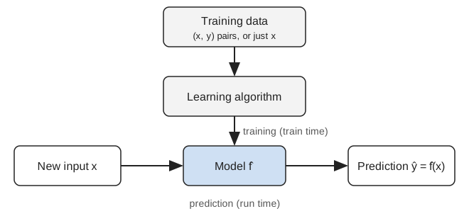
Figure 1: Training turns data into a model once; prediction applies the model to each new input.
Flow diagram.   Training data, made of (x, y) pairs or just x, flows into a learning algorithm, which produces a model f-hat;   this step is labeled training, at train time.   A new input x flows into the model f-hat, which outputs a prediction y-hat equal to f-hat of x;   this step is labeled prediction, at run time.

1.2 The three parts of a learning problem

ExrExercise 1 (What are the parts of a learning problem?)

Exercise 1 (What are the parts of a learning problem?) Figure 1 shows training and then prediction. Name the three objects that training involves:

  • what goes in;
  • what does the computation;
  • what comes out.

Solution 1. Training involves three objects:

  • data go in;
  • an algorithm does the computation;
  • a rule for making predictions comes out.
DefDefinition 1 (Training data (training set))

Definition 1 (Training data (training set)) The training data are inputs \(x\), possibly with outputs \(y\).

Other names: the training data are also called the training set.

DefDefinition 2 (Learning algorithm)

Definition 2 (Learning algorithm) A learning algorithm turns the training data (Definition 1) into a function \(h\).

DefDefinition 3 (Training (fitting, learning, estimation))

Definition 3 (Training (fitting, learning, estimation)) Running a learning algorithm (Definition 2) on the training data is called training.

Other names: training is also called fitting, learning or estimation.

DefDefinition 4 (Feature (attribute))

Definition 4 (Feature (attribute)) A feature is one number that a model family receives as input [1]: one entry of the output of the preprocessing applied to an input’s covariates. With no preprocessing, the features are the covariates.

Other names: a feature is also called an attribute. A covariate, a predictor, an input variable and an independent variable are the measured values before preprocessing.

DefDefinition 5 (Model)

Definition 5 (Model) A model is a set of candidate descriptions of how the outcomes of a data set depend on its inputs, or one member of such a set that training has chosen.

RemarkRemark 1 (A model represents a phenomenon)

Remark 1 (A model represents a phenomenon). In science, a model represents an object, a phenomenon or a process, and it makes some part of the world easier to understand, quantify or simulate [2], [3]. The candidates in a model represent how the outcomes of a data set depend on its inputs. Choosing the set of candidates is an assumption: the set rules out every description outside it. George Box summed up what that assumption costs as “all models are wrong but some are useful” [4, p. 202]. He argued that no simple model represents a system in the world exactly, but a well-chosen simple model can still approximate it usefully, as the ideal gas law \(PV = RT\) does for actual gases, none of which obeys it exactly [4, pp. 202–203]. So the question to ask of a model is not whether it is true. In his words, the question is “Is the model illuminating and useful?” [4, p. 203]. Box also noted that a method derived without an explicitly stated model still implies some unstated model [4, p. 201], so even a method that only makes predictions rests on assumptions about the data. A conceptual model is the same idea outside mathematics: a representation of a system, built from concepts, that helps people understand it.

DefDefinition 6 (Statistical model)

Definition 6 (Statistical model) A statistical model is a model whose candidates are distribution models: either a distribution model family or a fitted distribution model.

DefDefinition 7 (Predictive model)

Definition 7 (Predictive model) A predictive model is a model whose candidates are the members of a prediction function family: either the family itself or one member of the family that training has chosen.

ExmExample 1 (Gaussian outcomes with an affine mean: a model of both kinds)

Example 1 (Gaussian outcomes with an affine mean: a model of both kinds) Take the set of distribution models that give an outcome \(\Outvar\), given a covariate value \(\predvar\), a Gaussian distribution whose mean is an affine function of \(\predvar\). That set is a statistical model. Each member also gives a mean function, and that function predicts the outcome at each covariate value. So the same assumptions also make a predictive model. Figure 2 draws one member.

Show code
intercept <- 1
slope <- 0.5
noise_sd <- 1
x_at <- c(2, 5, 8)
y_grid <- seq(-3, 3, length.out = 101)
curves <- tidyr::expand_grid(x_at = x_at, dev = y_grid)
curves <- dplyr::mutate(
  curves,
  y = intercept + slope * x_at + dev,
  density = dnorm(dev, sd = noise_sd),
  x = x_at + 2 * density
)
x_limits <- c(0, 10)
y_limits <- c(-2, 9)
curves |>
  ggplot2::ggplot() +
  ggplot2::aes(x = x, y = y, group = x_at) +
  ggplot2::geom_abline(
    intercept = intercept,
    slope = slope,
    colour = "#0072B2"
  ) +
  ggplot2::geom_path(colour = "#D55E00") +
  ggplot2::coord_cartesian(xlim = x_limits, ylim = y_limits) +
  ggplot2::labs(x = "covariate value x", y = "outcome y")
Show code
import matplotlib.pyplot as plt
import numpy as np

intercept, slope, noise_sd = 1, 0.5, 1
dev = np.linspace(-3, 3, 101)
density = np.exp(-0.5 * (dev / noise_sd) ** 2) / (noise_sd * np.sqrt(2 * np.pi))
x_line = np.array([0, 10])
fig, ax = plt.subplots(figsize=(5, 3.5), layout="constrained")
ax.plot(x_line, intercept + slope * x_line, color="#0072B2");
for x_at in [2, 5, 8]:
    ax.plot(x_at + 2 * density, intercept + slope * x_at + dev, color="#D55E00");
ax.set_xlim(0, 10);
ax.set_ylim(-2, 9);
ax.set_xlabel("covariate value x");
ax.set_ylabel("outcome y");
plt.show()
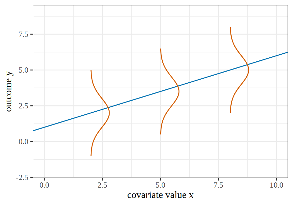
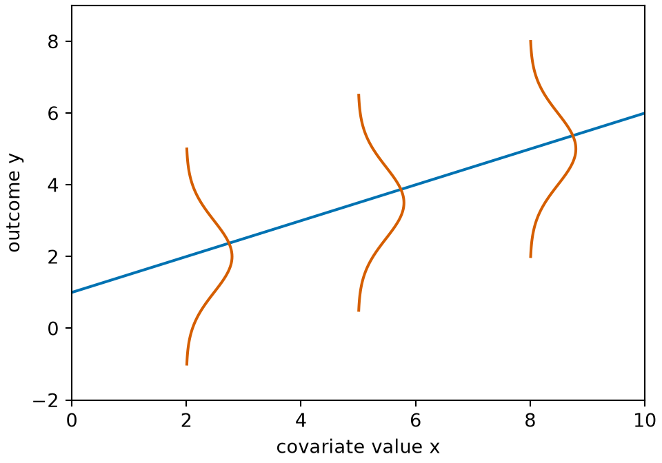
Figure 2: One member of the statistical model in Example 1: the Gaussian distributions of \(\Outvar\) given \(\predvar = 2\), \(5\) and \(8\), centered on the line \(\outvar = 1 + 0.5 \predvar\), each with standard deviation \(1\).
(a)
Line chart of one member of a statistical model. A blue line rises from y equals 1 at x equals 0 to y equals 6 at x equals 10. At x equals 2, 5 and 8, a vermilion bell curve drawn sideways, centered on the line, shows the Gaussian distribution that the member gives the outcome at that covariate value.
(b)
Line chart of one member of a statistical model. A blue line rises from y equals 1 at x equals 0 to y equals 6 at x equals 10. At x equals 2, 5 and 8, a vermilion bell curve drawn sideways, centered on the line, shows the Gaussian distribution that the member gives the outcome at that covariate value.
RemarkRemark 2 (Causal models are a third kind)

Remark 2 (Causal models are a third kind). A causal model is a further kind of model. Its candidates also describe how the distribution of the data would change under an intervention, such as setting one variable to a chosen value. So a causal model carries a statistical model with it, but a statistical model says nothing about interventions. These notes do not use causal models.

RemarkRemark 3 (Which meaning of “model” these notes use)

Remark 3 (Which meaning of “model” these notes use). A use of the word model names either a set of candidates or one chosen member, and the surrounding sentence shows which one. These notes usually use the word for a predictive model that training has chosen: the function \(\fitmodf{\trainset}\) that training produces from the training data \(\trainset\) and a prediction function family. The chosen function turns a new input value \(\newpredval\) into the prediction \(\fitmodvalf{\trainset}{\newpredval}\). The input value \(\newpredval\) holds one value of each feature. The hat in \(\fitmodf{\trainset}\) marks a function estimated from data.

RemarkRemark 4 (“Predictor” can name a model)

Remark 4 (“Predictor” can name a model). Statistics uses predictor for a measured value of an input, a covariate. Some machine learning texts use the same word for a fitted model. Hastie, Tibshirani and Friedman call the averaged forest function “the random forest (regression) predictor” [5], equation 15.2. Murphy calls the function obtained by training on a subset of the data “the predictor” [6], equation 16.104. These notes use predictor only for a measured value of an input.

ExmExample 2 (The parts of the spam cutoff problem)

Example 2 (The parts of the spam cutoff problem) Name the parts of the spam cutoff rule on the Spambase data [7]: the training data (Definition 1) are the \((x, y)\) pairs of half the messages, the learning algorithm (Definition 2) is a function that searches cutoffs, training (Definition 3) is running it, and the model (Definition 5) is the rule it returns.

import numpy as np
import pandas as pd

spam_tp = pd.read_csv("data/spambase.csv")
n_tp = len(spam_tp)
order_tp = (np.arange(n_tp) * 1009) % n_tp  # scrambled row order, as before
train_tp, new_tp = order_tp[: n_tp // 2], order_tp[n_tp // 2 :]

# Training data: x is the share of "!" characters, y the label (1 = spam).
x_tp = spam_tp["char_freq_!"].to_numpy()
y_tp = spam_tp["Class"].to_numpy()

def learn_cutoff_tp(x, y):
    # The learning algorithm: turn training data into a cutoff.
    grid = np.round(np.arange(0, 3.01, 0.05), 2)
    return grid[np.argmin([np.mean((x > c) != (y == 1)) for c in grid])]

cut_tp = learn_cutoff_tp(x_tp[train_tp], y_tp[train_tp])  # training

def model_tp(x):
    # The model: map a new input x to a prediction.
    return (x > cut_tp).astype(int)

print("cutoff:", cut_tp)
cutoff: 0.1
print(pd.DataFrame({"x": x_tp[new_tp[:5]], "prediction": model_tp(x_tp[new_tp[:5]]),
                    "label": y_tp[new_tp[:5]]}))
       x  prediction  label
0  1.103           1      1
1  0.000           0      0
2  0.000           0      0
3  0.633           1      1
4  0.443           1      1
spam_tp <- read.csv("data/spambase.csv", check.names = FALSE)
n_tp <- nrow(spam_tp)
order_tp <- ((seq_len(n_tp) - 1) * 1009) %% n_tp + 1  # scrambled row order, as before
train_tp <- order_tp[seq_len(n_tp %/% 2)]
new_tp <- order_tp[-seq_len(n_tp %/% 2)]

# Training data: x is the share of "!" characters, y the label (1 = spam).
x_tp <- spam_tp[["char_freq_!"]]
y_tp <- spam_tp[["Class"]]

learn_cutoff_tp <- function(x, y) {
  # The learning algorithm: turn training data into a cutoff.
  grid <- round(seq(0, 3, by = 0.05), 2)
  grid[which.min(sapply(grid, function(c) mean((x > c) != (y == 1))))]
}

cut_tp <- learn_cutoff_tp(x_tp[train_tp], y_tp[train_tp])  # training

# The model: map a new input x to a prediction.
model_tp <- function(x) as.integer(x > cut_tp)

cat("cutoff:", cut_tp, "\n")
cutoff: 0.1 
five_tp <- new_tp[1:5]
data.frame(x = x_tp[five_tp], prediction = model_tp(x_tp[five_tp]), label = y_tp[five_tp])

Training on 2300 messages produced the model “spam when ! makes up more than 0.1% of the characters”. The model never saw the five messages printed, and it gets 5 of them right. The same algorithm, trained on different data, can return a different model.

VideosWatch

Abu-Mostafa names the components of a learning problem in his first Caltech lecture, from 3:06, and then formalizes them, from 12:47 [8], Lecture 1.

1.3 Inputs: feature vectors

ExrExercise 2 (How can an email be an input?)

Exercise 2 (How can an email be an input?) A learning algorithm computes with numbers. How could you describe one email, or one car, so that a learning algorithm can use it as an input?

Solution 2. Measure a list of properties, and write each one as a number: for an email, how often each of several words appears; for a car, its horsepower, weight and number of cylinders.

DefDefinition 8 (Feature vector)

Definition 8 (Feature vector) A feature vector \(x \in \reals^{\ninputvars}\) describes one input by \(\ninputvars\) features (Definition 4), one per measured property. It is an element of the real coordinate space \(\reals^{\ninputvars}\).

ExmExample 3 (A column and a row of Spambase)

Example 3 (A column and a row of Spambase) In the Spambase table [7], each column except Class is a feature (Definition 4): word_freq_free is the percentage of a message’s words that are free. A message’s feature vector is its row of those columns.

import pandas as pd

spam_fv = pd.read_csv("data/spambase.csv")
feats_fv = spam_fv.drop(columns="Class")  # the features; Class is the label y

# One feature: a column, with one value per message.
print(feats_fv["word_freq_free"].head(3))
0    0.32
1    0.14
2    0.06
Name: word_freq_free, dtype: float64
# One feature vector: a row, with one value per feature.
x1_fv = feats_fv.iloc[0].to_numpy()
print(x1_fv[:6])
[0.   0.64 0.64 0.   0.32 0.  ]
print("D =", len(x1_fv))
D = 57
spam_fv <- read.csv("data/spambase.csv", check.names = FALSE)
feats_fv <- spam_fv[, names(spam_fv) != "Class"]  # the features; Class is the label y

# One feature: a column, with one value per message.
head(feats_fv[["word_freq_free"]], 3)
[1] 0.32 0.14 0.06
# One feature vector: a row, with one value per feature.
x1_fv <- unlist(feats_fv[1, ], use.names = FALSE)
x1_fv[1:6]
[1] 0.00 0.64 0.64 0.00 0.32 0.00
cat("D =", length(x1_fv), "\n")
D = 57 

The feature word_freq_free has 4601 values, one per message. The first message’s feature vector has \(\ninputvars = 57\) entries, one per feature, so \(x \in \reals^{57}\) (Definition 8).

VideosWatch

Weinberger introduces feature vectors, from 33:27 [9], Lecture 1.

DefDefinition 9 (Feature function (feature map, encoding))

Definition 9 (Feature function (feature map, encoding)) A feature function \(\vfeatmap\) sends a covariate vector \(\vpredvar\), whose entries may be numbers or categories, to its feature vector (Definition 8) \(\vfeatmap(\vpredvar) \in \reals^{\ninputvars \times 1}\).

ExmExample 4 (Encoding a shelf location in the Carseats data)

Example 4 (Encoding a shelf location in the Carseats data) In the Carseats data [10], a store’s covariate vector holds its shelf location, a category (Bad, Medium or Good), and its price, a number. The feature function replaces the category with one 0/1 feature per category and keeps the price. The first three stores’ feature vectors are the rows below, so \(\ninputvars\) is the number of columns.

carseats <- read.csv("data/carseats.csv")[1:3, c("ShelveLoc", "Price")]
carseats$ShelveLoc <- factor(carseats$ShelveLoc, levels = c("Bad", "Medium", "Good"))
carseats
# One 0/1 column per shelf location, then the price.
data.frame(model.matrix(~ 0 + ShelveLoc + Price, data = carseats))
DefDefinition 10 (Output variable (label, target, response, outcome, dependent variable))

Definition 10 (Output variable (label, target, response, outcome, dependent variable)) The output variable is the quantity a supervised model predicts for an input. Each example has one value of it, written \(\outvar\) once observed; before it is observed, it is a random variable, written \(\Outvar\). In regression the output is a number, and in classification it is a class.

Other names: the output is also called the label, target, response, outcome or dependent variable. The term outcome is common in statistics and the term target in machine learning.

ExmExample 5 (The output of Spambase)

Example 5 (The output of Spambase) In the Spambase table [7], the Class column is the output variable (Definition 10): it is 1 for a message that is spam and 0 for one that is not. The other columns are the features (Definition 4).

import pandas as pd

spam_out = pd.read_csv("data/spambase.csv")
y_out = spam_out["Class"]  # the output variable: one value per message

# The output is a class, so count the messages in each class.
print(y_out.value_counts())
Class
0    2788
1    1813
Name: count, dtype: int64
spam_out <- read.csv("data/spambase.csv", check.names = FALSE)
y_out <- spam_out[["Class"]]  # the output variable: one value per message

# The output is a class, so count the messages in each class.
table(y_out)
y_out
   0    1 
2788 1813 

Of the 4601 messages, 1813 are spam, so the output takes the value 1 for 39.4% of them.

Most often, each input is a feature vector.

ExrExercise 3 (How long is the feature vector?)

Exercise 3 (How long is the feature vector?) What is \(\ninputvars\) for each of these inputs?

An email in the spam data, described by the relative frequencies of 57 words and characters.

Solution 3. \(\ninputvars = 57\): one relative frequency per word or character.

ExrExercise 4 (How long is the feature vector? (part 2))

Exercise 4 (How long is the feature vector? (part 2)) Use the setup of Exercise 3.

A handwritten ZIP-code digit, scanned as a 16-by-16 grid of grayscale pixels.

Solution 4. One intensity per pixel:

\[ \begin{aligned} \ninputvars &= 16 \times 16 \\ &= 256. \end{aligned} \]

ExrExercise 5 (Does every input fit in a row?)

Exercise 5 (Does every input fit in a row?) Consider four inputs:

  • one car, described by its engine size, weight and fuel economy;
  • the text of an email;
  • a color photograph;
  • a recorded spoken sentence.

Which of them arrive as a fixed list of attributes, and which do not?

Solution 5. Only the car arrives as a fixed list of attributes. Tabular data like it is structured; text, images and audio are unstructured.

ExrExercise 6 (Does every input fit in a row? (part 2))

Exercise 6 (Does every input fit in a row? (part 2)) Use the setup of Exercise 5.

For each one that does not, name a form in which a model could receive it.

Solution 6. An unstructured input can be presented to a model in several forms:

  • flattened into a \(\ninputvars\)-vector for a classical model, as the scanned digit was in Exercise 4;
  • kept as a multi-dimensional array for a model that takes grid-shaped input directly: a matrix \(\predvar \in \reals^{D_1 \times D_2}\) for a grayscale image or a spectrogram, or a 3-D array for the color photograph;
  • given as a sequence of inputs, as for the spoken sentence or the email’s words;
  • structured as an object, such as a parse tree of the email’s sentences.
DefDefinition 11 (Structured data)

Definition 11 (Structured data) Data are structured when every observation is described by the same fixed list of attributes, so a dataset of them fits in a table with one row per observation and one column per attribute.

Example: a list of cars, each described by its engine size, weight and fuel economy.

DefDefinition 12 (Unstructured data)

Definition 12 (Unstructured data) Data are unstructured when they do not come as a fixed list of attributes: a model receives the raw content, such as words, pixels or audio samples, and any attributes have to be derived from it.

Examples: the text of an email, a photograph, a recorded sentence.

ExmExample 6 (The numbers and the names in the Auto table)

Example 6 (The numbers and the names in the Auto table) The Auto data [10] describe each car by the same fixed list of attributes: mpg, cylinders, displacement, horsepower, weight, acceleration, year and origin. The last column, name, is free text:

import pandas as pd

auto_sd = pd.read_csv("data/auto.csv")
# Structured: every car has the same attributes, so the data fit a table.
print(auto_sd.drop(columns="name").head(3))
    mpg  cylinders  displacement  ...  acceleration  year  origin
0  18.0          8         307.0  ...          12.0    70       1
1  15.0          8         350.0  ...          11.5    70       1
2  18.0          8         318.0  ...          11.0    70       1

[3 rows x 8 columns]
# Unstructured: the text of a name has no fixed attributes. To use it,
# we derive one, here the make, which we take to be the first word.
make_sd = auto_sd["name"].str.split().str[0]
print(auto_sd["name"].head(3).tolist())
['chevrolet chevelle malibu', 'buick skylark 320', 'plymouth satellite']
print(make_sd.value_counts().head(3))
name
ford         48
chevrolet    43
plymouth     31
Name: count, dtype: int64
auto_sd <- read.csv("data/auto.csv")
# Structured: every car has the same attributes, so the data fit a table.
head(auto_sd[, names(auto_sd) != "name"], 3)
# Unstructured: the text of a name has no fixed attributes. To use it,
# we derive one, here the make, which we take to be the first word.
make_sd <- sapply(strsplit(auto_sd$name, " "), `[`, 1)
head(auto_sd$name, 3)
[1] "chevrolet chevelle malibu" "buick skylark 320"        
[3] "plymouth satellite"       
head(sort(table(make_sd), decreasing = TRUE), 3)
make_sd
     ford chevrolet  plymouth 
       48        43        31 

The numeric columns of the 392 cars are structured data (Definition 11): every row has the same 8 attributes. The name text is unstructured (Definition 12) until we derive an attribute from it, and the make we derived takes 37 distinct values. A derived attribute inherits the text’s quirks: chevrolet, chevy and chevroelt count as three makes.

An unstructured input can reach a model in several forms: flattened into a \(\ninputvars\)-vector, kept as a multi-dimensional array, given as a sequence, or structured as an object such as a parse tree; Solution 5 gives an example of each.

Historically, turning unstructured data (Definition 12) into good features was a large part of applied machine learning. Hand-engineered features create an information bottleneck: any attribute left out of the feature vector is lost to the model, and the choice of features reflects what its designers overlooked. Deep learning architectures, such as convolutional and recurrent networks, avoid the bottleneck by taking raw inputs and learning feature representations from them. Categorical inputs, such as a color, are turned into numbers too, for example by one-hot encoding (Harris’ 2022 weekly notes).

ExrExercise 7 (Explore a real dataset)

Exercise 7 (Explore a real dataset) The plot shows the cars of the Auto data from the Introduction to Statistical Learning labs [10], [11]. Pick what to plot. Which variable would you most want to predict from the others, and which variables would you predict it from?

Show code
viewof autoX = Inputs.select(autoVars, {value: "horsepower", label: "x"})
viewof autoY = Inputs.select(autoVars, {value: "mpg", label: "y"})
viewof autoColor = Inputs.select(autoVars, {value: "origin", label: "color by"})
Show code
Plot.plot({
  ariaLabel: 'Scatter plot of the Auto cars, with the x, y and color variables chosen from the controls; by default mpg against horsepower, colored by origin.',
  height: 320, width: 760, grid: true,
  x: {label: autoX}, y: {label: autoY},
  color: {legend: true, label: autoColor,
          type: autoColor === "origin" || autoColor === "cylinders" ? "ordinal" : "linear",
          scheme: autoColor === "origin" || autoColor === "cylinders" ? "category10" : "viridis"},
  marks: [Plot.dot(auto, {x: autoX, y: autoY, fill: autoColor, r: 3,
                          fillOpacity: 0.8, tip: true, title: "name"})]
})
Figure 3: Any two Auto variables plotted against each other, colored by a third.

In origin, 1 is American, 2 is European and 3 is Japanese.
Solution 7. There is no single right answer. Two natural choices:

  • Predict mpg from horsepower, weight and the rest. Plotting mpg against horsepower (Figure 4) shows mpg falling as horsepower rises, and along a curve rather than a straight line.
  • Predict origin from the rest. The colors in Figure 4 show that the European and Japanese cars differ from the American ones in both mpg and horsepower.
Figure 4: Miles per gallon against horsepower for the cars of the Auto data, colored by origin. The black curve is a loess smooth of all the cars.

2 Kinds of learning problems

2.1 Supervised and unsupervised learning

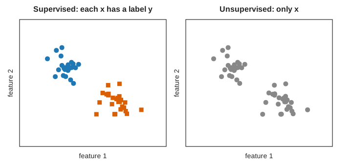
Figure 5: The same fifty points, with labels (left) and without (right). A classifier learns to separate the labeled groups; a clustering algorithm must find the groups without labels.
Two scatter plots of the same fifty points in two dimensions. On the left, titled Supervised: each x has a label y, the points are colored by label: a blue cluster of circles at upper left and an orange cluster of squares at lower right. On the right, titled Unsupervised: only x, the same points are all gray.
ExrExercise 8 (What differs between the two panels?)

Exercise 8 (What differs between the two panels?) The two panels of Figure 5 show the same fifty points. What does the left panel give a learning algorithm that the right panel does not?

Solution 8. The left panel gives the group of every point, and the right panel gives only the points.

ExrExercise 9 (What differs between the two panels? (part 2))

Exercise 9 (What differs between the two panels? (part 2)) Use the setup of Exercise 8.

What could the goal be in each of the two panels?

Solution 9. With the group of every point, the goal could be to predict the group of a new point. With only the points, the goal could be to find groups among them.

DefDefinition 13 (Supervised learning)

Definition 13 (Supervised learning) In supervised learning, every training example is a pair \((\vpredvar, \outvar)\): the correct output is given, and the goal is to predict \(\outvar\) for new \(\vpredvar\) [12].

Here \(\outvar\) is the output variable (Definition 10), which has other names there. A training example is also called an observation or an instance.

DefDefinition 14 (Unsupervised learning)

Definition 14 (Unsupervised learning) In unsupervised learning, the training data are inputs \(x\) alone, and the goal is to find structure in them, such as groups, directions of variation, or a density [13].

ExmExample 7 (The Spambase table with and without its labels)

Example 7 (The Spambase table with and without its labels) Take three feature columns of Spambase [7], and the Class column that labels each message. With Class, the table holds \((x, y)\) pairs. Without it, the table holds inputs \(x\) alone.

import pandas as pd

spam_su = pd.read_csv("data/spambase.csv")
feats_su = ["word_freq_free", "word_freq_you", "char_freq_!"]

# Supervised: each row is a pair (x, y), and the goal is to predict y from x.
# Comparing the label groups shows which features carry information about y.
print(spam_su[feats_su + ["Class"]].head(3))
   word_freq_free  word_freq_you  char_freq_!  Class
0            0.32           1.93        0.778      1
1            0.14           3.47        0.372      1
2            0.06           1.36        0.276      1
print(spam_su.groupby("Class")[feats_su].mean().round(2))
       word_freq_free  word_freq_you  char_freq_!
Class                                            
0                0.07           1.27         0.11
1                0.52           2.26         0.51
# Unsupervised: drop the labels and look for structure in x alone,
# here which features rise and fall together.
print(spam_su[feats_su].corr().round(2))
                word_freq_free  word_freq_you  char_freq_!
word_freq_free            1.00           0.08         0.10
word_freq_you             0.08           1.00         0.15
char_freq_!               0.10           0.15         1.00
spam_su <- read.csv("data/spambase.csv", check.names = FALSE)
feats_su <- c("word_freq_free", "word_freq_you", "char_freq_!")

# Supervised: each row is a pair (x, y), and the goal is to predict y from x.
# Comparing the label groups shows which features carry information about y.
head(spam_su[, c(feats_su, "Class")], 3)
aggregate(spam_su[, feats_su], by = list(Class = spam_su$Class), FUN = mean)
# Unsupervised: drop the labels and look for structure in x alone,
# here which features rise and fall together.
round(cor(spam_su[, feats_su]), 2)
               word_freq_free word_freq_you char_freq_!
word_freq_free           1.00          0.08        0.10
word_freq_you            0.08          1.00        0.15
char_freq_!              0.10          0.15        1.00

In the supervised view (Definition 13), spam averages 0.52% free against 0.07% in email, so free helps predict the label. In the unsupervised view (Definition 14) there is no label to predict: the only finding is structure in the inputs, such as a correlation of 0.08 between free and you.

VideosWatch

Hastie and Tibshirani present the supervised learning problem, then unsupervised learning, from 4:02 [14], video 1.2.

ReadingRead

GeeksforGeeks explains supervised and unsupervised learning [15].

ExrExercise 10 (What if labels are scarce, or there are none?)

Exercise 10 (What if labels are scarce, or there are none?) Suppose only a few of the training examples have labels. A harder case: no one gives the correct answer at all, and a game program learns only whether it won. What kind of learning does each case call for?

Solution 10. An algorithm given a few labels could learn from the labeled and the unlabeled examples together. A program given no correct answers could learn from the results of its own moves, counting a win as good and a loss as bad.

DefDefinition 15 (Semi-supervised learning)

Definition 15 (Semi-supervised learning) In semi-supervised learning, the training data hold a few labeled examples and many unlabeled ones [16]. For a spam filter, the labeled examples are the emails someone has read and marked as spam or email; the rest of the inbox is unlabeled.

ExmExample 8 (A spam filter with 100 labeled messages)

Example 8 (A spam filter with 100 labeled messages) Suppose only 100 of the Spambase messages [7] have been read and marked as spam or email, and the rest of the inbox is unlabeled.

import numpy as np
import pandas as pd

spam_ss = pd.read_csv("data/spambase.csv")
n_ss = len(spam_ss)
order_ss = (np.arange(n_ss) * 1009) % n_ss  # scrambled row order, as before

# Hide every label except those of the first 100 messages in the scrambled order.
y_ss = np.array(spam_ss["Class"], dtype=float)  # a writable copy
y_ss[order_ss[100:]] = np.nan
print("labeled:", int(np.sum(~np.isnan(y_ss))), " unlabeled:", int(np.sum(np.isnan(y_ss))))
labeled: 100  unlabeled: 4501
# Every message still has its features; only the labeled ones can score a cutoff.
x_ss = spam_ss["char_freq_!"].to_numpy()
lab_ss = ~np.isnan(y_ss)
grid_ss = np.round(np.arange(0, 3.01, 0.05), 2)
errs_ss = [np.mean((x_ss[lab_ss] > c) != (y_ss[lab_ss] == 1)) for c in grid_ss]
cut_ss = grid_ss[np.argmin(errs_ss)]

# Check it against the labels we hid.
truth_ss = spam_ss["Class"].to_numpy()[~lab_ss]
print("cutoff:", cut_ss, " error on the unlabeled:",
      round(np.mean((x_ss[~lab_ss] > cut_ss) != (truth_ss == 1)), 3))
cutoff: 0.05  error on the unlabeled: 0.217
spam_ss <- read.csv("data/spambase.csv", check.names = FALSE)
n_ss <- nrow(spam_ss)
order_ss <- ((seq_len(n_ss) - 1) * 1009) %% n_ss + 1  # scrambled row order, as before

# Hide every label except those of the first 100 messages in the scrambled order.
y_ss <- spam_ss$Class
y_ss[order_ss[-seq_len(100)]] <- NA
missing_ss <- is.na(y_ss)
n_unlab_ss <- sum(missing_ss)
n_lab_ss <- length(y_ss) - n_unlab_ss
cat("labeled:", n_lab_ss, " unlabeled:", n_unlab_ss, "\n")
labeled: 100  unlabeled: 4501 
# Every message still has its features;
# only the labeled ones can score a cutoff.
x_ss <- spam_ss[["char_freq_!"]]
lab_ss <- !is.na(y_ss)
grid_ss <- round(seq(0, 3, by = 0.05), 2)
errs_ss <- sapply(grid_ss, function(c) mean((x_ss[lab_ss] > c) != (y_ss[lab_ss] == 1)))
cut_ss <- grid_ss[which.min(errs_ss)]

# Check it against the labels we hid.
truth_ss <- spam_ss$Class[!lab_ss]
cat("cutoff:", cut_ss, " error on the unlabeled:",
    round(mean((x_ss[!lab_ss] > cut_ss) != (truth_ss == 1)), 3), "\n")
cutoff: 0.05  error on the unlabeled: 0.217 

The training data hold 100 labeled examples and 4501 unlabeled ones (Definition 15). This code uses only the labeled 100 to choose the cutoff, so the 4501 unlabeled messages go unused. A semi-supervised method would also learn from their features. The hidden labels were used above only to check the result.

DefDefinition 16 (Reinforcement learning)

Definition 16 (Reinforcement learning) In reinforcement learning, an agent acts and learns from rewards rather than from correct answers [17]. For a program learning to play a board game, for example, its actions are its moves, and its reward comes from how its games turn out, not from a label saying which move was right.

ExmExample 9 (A filter that learns only from rewards)

Example 9 (A filter that learns only from rewards) Let a spam filter act on the Spambase messages [7] one at a time: its action is to send each message to the junk folder or to the inbox, and the only feedback is a reward, +1 for a right call and -1 for a wrong one. Try three cutoff policies, each on its own 500 messages, and keep the one with the highest average reward:

import numpy as np
import pandas as pd

spam_rl = pd.read_csv("data/spambase.csv")
n_rl = len(spam_rl)
order_rl = (np.arange(n_rl) * 1009) % n_rl  # scrambled message order, as before
x_rl = spam_rl["char_freq_!"].to_numpy()
y_rl = spam_rl["Class"].to_numpy()

def reward_rl(cut, rows):
    # Act: junk the message if x > cut. The environment returns +1 or -1;
    # the learner keeps these rewards, not the labels behind them.
    return np.where((x_rl[rows] > cut) == (y_rl[rows] == 1), 1, -1)

for j, cut in enumerate([0.05, 0.5, 1.5]):
    rows = order_rl[500 * j : 500 * (j + 1)]
    print("cutoff", cut, "mean reward:", round(reward_rl(cut, rows).mean(), 3))
cutoff 0.05 mean reward: 0.576
cutoff 0.5 mean reward: 0.432
cutoff 1.5 mean reward: 0.248
spam_rl <- read.csv("data/spambase.csv", check.names = FALSE)
n_rl <- nrow(spam_rl)
order_rl <- ((seq_len(n_rl) - 1) * 1009) %% n_rl + 1  # scrambled message order, as before
x_rl <- spam_rl[["char_freq_!"]]
y_rl <- spam_rl$Class

reward_rl <- function(cut, rows) {
  # Act: junk the message if x > cut. The environment returns +1 or -1;
  # the learner keeps these rewards, not the labels behind them.
  ifelse((x_rl[rows] > cut) == (y_rl[rows] == 1), 1, -1)
}

cuts_rl <- c(0.05, 0.5, 1.5)
mean_reward_rl <- sapply(seq_along(cuts_rl), function(j) {
  mean(reward_rl(cuts_rl[j], order_rl[(500 * (j - 1) + 1):(500 * j)]))
})
for (j in seq_along(cuts_rl)) {
  cat("cutoff", cuts_rl[j], "mean reward:", round(mean_reward_rl[j], 3), "\n")
}
cutoff 0.05 mean reward: 0.576 
cutoff 0.5 mean reward: 0.432 
cutoff 1.5 mean reward: 0.248 

The policy with cutoff 0.05 earns the highest average reward, 0.58, so this agent would adopt it (Definition 16). This is the simplest case. In a game such as checkers, the reward arrives only when the game ends, and says nothing about which move was the mistake.

ReadingRead

Semi-supervised data are common, because labels cost time and money: someone has to read each email to mark it as spam, while unread emails arrive at no cost. The week 10 lecture on reinforcement learning replaces labels with rewards.

ExrExercise 11 (How could a computer find groups?)

Exercise 11 (How could a computer find groups?) A dataset has points with no labels, and we want \(k\) groups. Propose a procedure that a computer could repeat to split the points into \(k\) groups.

Solution 11. Start with a rough guess at the groups, then keep improving the guess:

  1. put each point with the group whose middle is closest;
  2. recompute each middle;
  3. stop once no point changes group.
DefDefinition 17 (Clustering)

Definition 17 (Clustering) Clustering is the unsupervised task (Definition 14) of dividing \(N\) inputs \(\vx_1, \ldots, \vx_N\) into groups, called clusters, so that inputs in the same cluster are more similar to each other than to inputs in other clusters [20]. The output is a cluster assignment for each input. No labels are given, so the clusters are found, not learned from examples of the right answer.

ExmExample 10 (Grouping cars without labels)

Example 10 (Grouping cars without labels) Ignore mpg and every other column of the Auto data [10] except two: the horsepower and weight of each car. Standardize both, so that neither dominates the distances, and cluster the cars into three groups by two methods, \(k\)-means and hierarchical clustering with Ward linkage. Cluster labels are arbitrary, so number the clusters from the lightest cars to the heaviest:

import numpy as np
import pandas as pd
from scipy.cluster.hierarchy import fcluster, linkage
from sklearn.cluster import KMeans

auto_cl = pd.read_csv("data/auto.csv").dropna(subset=["horsepower"])
x_cl = auto_cl[["horsepower", "weight"]].to_numpy(float)
x_cl = (x_cl - x_cl.mean(axis=0)) / x_cl.std(axis=0, ddof=1)
w_cl = auto_cl["weight"].to_numpy(float)

def by_weight(labels, weight):
    # Renumber the clusters 0, 1, 2 in order of their mean weight.
    ids, inverse = np.unique(labels, return_inverse=True)
    order = np.argsort([weight[labels == g].mean() for g in ids])
    return np.argsort(order)[inverse]

km_cl = by_weight(KMeans(3, n_init=10, random_state=1).fit(x_cl).labels_, w_cl)
hc_cl = by_weight(fcluster(linkage(x_cl, "ward"), 3, criterion="maxclust"), w_cl)

print(np.bincount(km_cl), np.bincount(hc_cl))
[159 138  95] [102 187 103]
print(pd.crosstab(km_cl, hc_cl))
col_0    0    1   2
row_0              
0      102   57   0
1        0  130   8
2        0    0  95
auto_cl <- na.omit(read.csv("data/auto.csv")[, c("horsepower", "weight")])
x_cl <- scale(auto_cl)

# Renumber the clusters 1, 2, 3 in order of their mean weight.
by_weight <- function(labels, weight) {
  rank(tapply(weight, labels, mean))[as.character(labels)]
}

set.seed(1)
km_fit <- kmeans(x_cl, centers = 3, nstart = 10)
km_cl <- by_weight(km_fit$cluster, auto_cl$weight)
hc_cl <- by_weight(cutree(hclust(dist(x_cl), "ward.D2"), k = 3), auto_cl$weight)

rbind(kmeans = table(km_cl), ward = table(hc_cl))
         1   2   3
kmeans 156 141  95
ward   102 187 103
table(kmeans = km_cl, ward = hc_cl)
      ward
kmeans   1   2   3
     1 102  54   0
     2   0 133   8
     3   0   0  95

Both methods split the 392 cars into light, middle and heavy groups, and neither was told which cars are which. \(k\)-means puts 156, 141 and 95 cars in them, Ward linkage 102, 187 and 103. They agree on 330 cars and differ on the other 62. Each method is an answer to the same task, clustering (Definition 17). The two languages start \(k\)-means differently, so their counts can differ slightly. The prose gives the R values.

Show code
library(ggplot2)
cl_long <- rbind(
  data.frame(auto_cl, method = "k-means", group = factor(km_cl)),
  data.frame(auto_cl, method = "Ward linkage", group = factor(hc_cl))
)
cl_long$method <- factor(cl_long$method, levels = c("k-means", "Ward linkage"))
ggplot(cl_long, aes(horsepower, weight, colour = group, shape = group)) +
  geom_point(alpha = 0.7) +
  scale_colour_manual(values = c("1" = "#0072B2", "2" = "#D55E00", "3" = "#009E73")) +
  scale_shape_manual(values = c("1" = 16, "2" = 17, "3" = 15)) +
  facet_wrap(~method) +
  labs(x = "Horsepower", y = "Weight (lb)", colour = "Group", shape = "Group")
Show code
import matplotlib.pyplot as plt

fig, axes = plt.subplots(1, 2, figsize=(7, 3.5), sharey=True, layout="constrained")
styles_cl = [("#0072B2", "o"), ("#D55E00", "^"), ("#009E73", "s")]
for ax, labels, title in zip(axes, [km_cl, hc_cl], ["k-means", "Ward linkage"]):
    for g, (colour, marker) in enumerate(styles_cl):
        keep = labels == g
        ax.plot(auto_cl["horsepower"][keep], auto_cl["weight"][keep], color=colour,
                marker=marker, linestyle="", alpha=0.7, label=f"group {g + 1}");
    ax.set_title(title);
    ax.set_xlabel("Horsepower");
axes[0].set_ylabel("Weight (lb)");
fig.legend(*axes[0].get_legend_handles_labels(), loc="outside lower center", ncol=3);
plt.show()
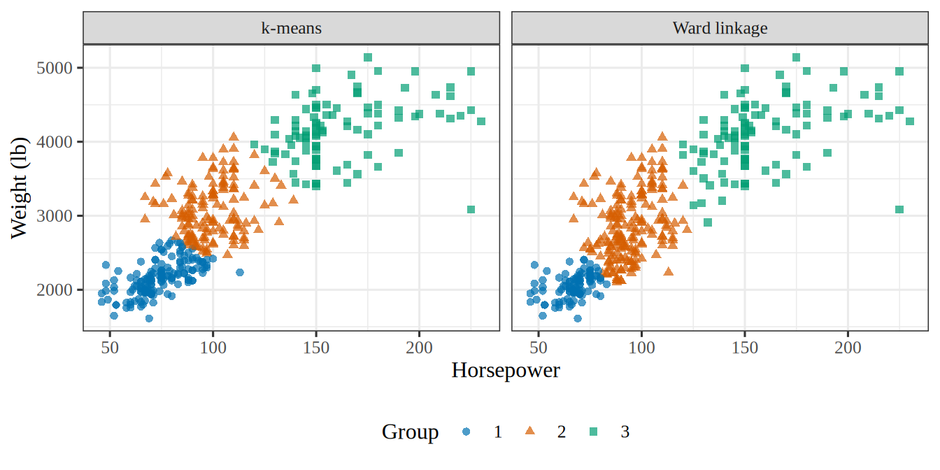
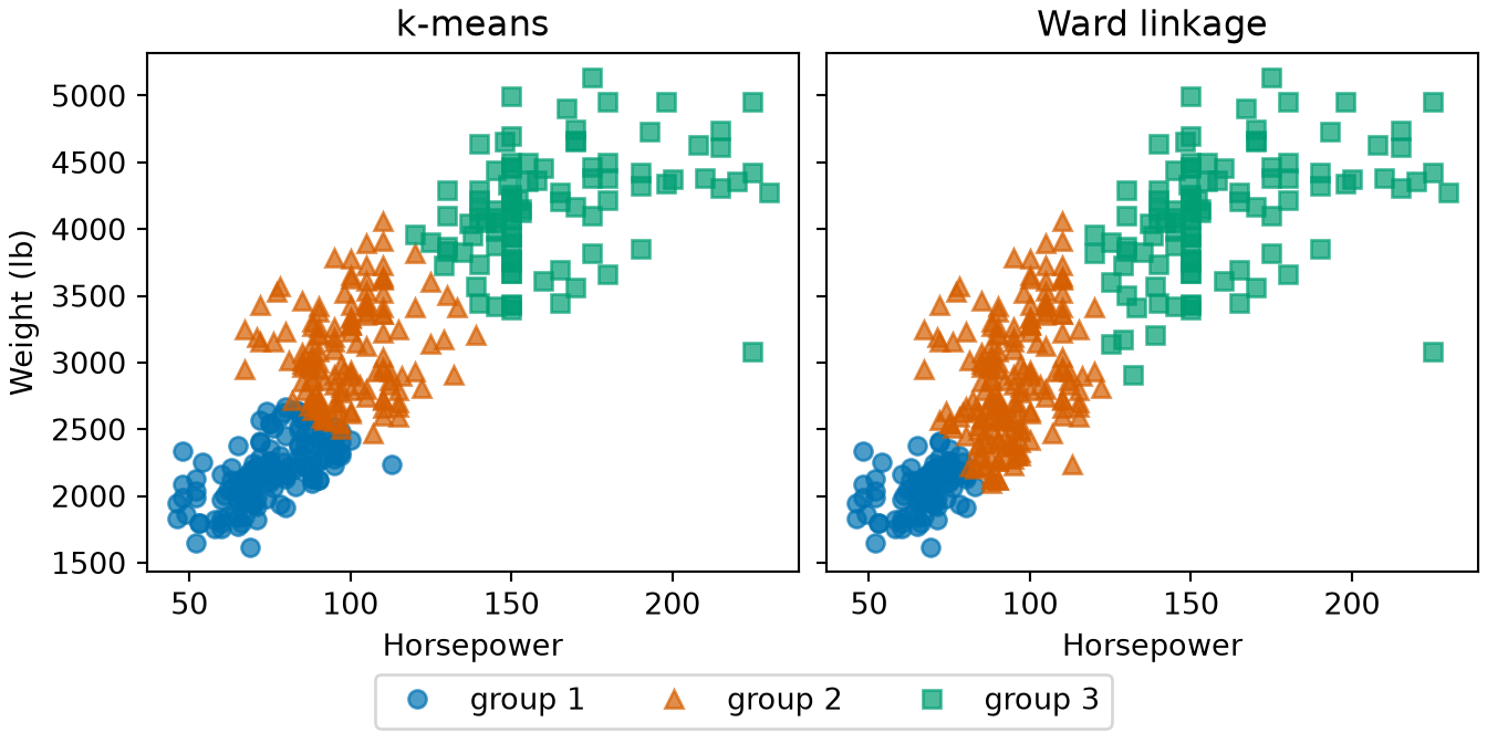
Figure 6: The cars of Example 10 by horsepower and weight, colored by the group that each method found. Both methods split the cars into light, middle and heavy groups.
(a)
Two scatter plots side by side of the weight of each car against its horsepower, one panel for the three groups found by k-means and one for the three groups found by Ward linkage. In both panels the cars run from light, low-power cars at the lower left to heavy, high-power cars at the upper right. Group 1, the lightest, is drawn as blue circles, group 2 as vermilion triangles and group 3, the heaviest, as green squares. The groups in the two panels cover nearly the same regions.
(b)
Two scatter plots side by side of the weight of each car against its horsepower, one panel for the three groups found by k-means and one for the three groups found by Ward linkage. In both panels the cars run from light, low-power cars at the lower left to heavy, high-power cars at the upper right. Group 1, the lightest, is drawn as blue circles, group 2 as vermilion triangles and group 3, the heaviest, as green squares. The groups in the two panels cover nearly the same regions.
RemarkRemark 5 (Clustering is a task, not an algorithm)

Remark 5 (Clustering is a task, not an algorithm). Clustering names the task, not a way of doing it. \(k\)-means (Definition 18) is one method for it, and hierarchical clustering is another, so the same inputs can be clustered in more than one way.

DefDefinition 18 (k-means)

Definition 18 (k-means) k-means is a classic method for clustering (Definition 17) the inputs into \(k\) groups [21]. It starts with \(k\) group centers and repeats two steps until the assignments stop changing:

  1. assign each point to its nearest center;
  2. move each center to the mean of the points assigned to it.
ExmExample 11 (Two groups among the Spambase messages)

Example 11 (Two groups among the Spambase messages) Run \(k\)-means with \(k = 2\) on two Spambase features [7], the percentages of ! and $ characters, without showing it the labels. Both percentages are heavy-tailed, so the code works with \(\log(1 + \text{percentage})\), which keeps a few extreme messages from taking over:

import numpy as np
import pandas as pd

spam_km = pd.read_csv("data/spambase.csv")
feat_km = np.log1p(spam_km[["char_freq_!", "char_freq_$"]].to_numpy())

# Start from the messages with the smallest and the largest feature total.
sums_km = feat_km.sum(axis=1)
centers_km = feat_km[[sums_km.argmin(), sums_km.argmax()]]

for _ in range(100):
    # Step 1: assign each point to its nearest center.
    dist_km = ((feat_km[:, None, :] - centers_km[None, :, :]) ** 2).sum(axis=2)
    group_km = dist_km.argmin(axis=1)
    # Step 2: move each center to the mean of its points; stop when nothing moves.
    new_km = np.array([feat_km[group_km == g].mean(axis=0) for g in range(2)])
    if np.allclose(new_km, centers_km):
        break
    centers_km = new_km

print(centers_km.round(2))
[[0.06 0.04]
 [0.64 0.16]]
# k-means never saw Class; compare its groups with it afterwards.
print(pd.crosstab(group_km, spam_km["Class"], rownames=["group"]))
Class     0     1
group            
0      2652  1025
1       136   788
spam_km <- read.csv("data/spambase.csv", check.names = FALSE)
feat_km <- log1p(as.matrix(spam_km[, c("char_freq_!", "char_freq_$")]))

# Start from the messages with the smallest and the largest feature total.
sums_km <- rowSums(feat_km)
start_km <- feat_km[c(which.min(sums_km), which.max(sums_km)), ]

# kmeans() repeats the assign and move steps; "Lloyd" is the version
# described in the definition.
fit_km <- kmeans(feat_km, centers = start_km, algorithm = "Lloyd", iter.max = 100)
round(fit_km$centers, 2)
  char_freq_! char_freq_$
1        0.06        0.04
2        0.64        0.16
# k-means never saw Class; compare its groups with it afterwards.
tab_km <- table(group = fit_km$cluster, Class = spam_km$Class)
tab_km
     Class
group    0    1
    1 2652 1025
    2  136  788

The groups hold 3677 and 924 messages. The method used only the features, as an unsupervised method does (Definition 14), yet 85% of the messages in group 2 are spam, against 28% in group 1. Groups found without labels can still line up with the labels.

Show code
library(ggplot2)
km_points <- data.frame(
  excl = feat_km[, 1], dollar = feat_km[, 2],
  group = factor(fit_km$cluster)
)
km_centers <- data.frame(excl = fit_km$centers[, 1], dollar = fit_km$centers[, 2])
ggplot(km_points, aes(excl, dollar, colour = group, shape = group)) +
  geom_point(alpha = 0.4) +
  geom_point(data = km_centers, shape = 4, size = 4, stroke = 1.5, colour = "black") +
  scale_colour_manual(values = c("1" = "#0072B2", "2" = "#D55E00")) +
  scale_shape_manual(values = c("1" = 16, "2" = 17)) +
  labs(
    x = "Log of one plus the percentage of !",
    y = "Log of one plus the percentage of $",
    colour = "Group", shape = "Group"
  )
Show code
import matplotlib.pyplot as plt

fig, ax = plt.subplots(figsize=(5, 4), layout="constrained")
for g, (colour, marker) in enumerate([("#0072B2", "o"), ("#D55E00", "^")]):
    keep = group_km == g
    ax.plot(feat_km[keep, 0], feat_km[keep, 1], color=colour, marker=marker,
            linestyle="", alpha=0.4, label=f"group {g + 1}");
ax.plot(centers_km[:, 0], centers_km[:, 1], color="black", marker="x", markersize=10,
        markeredgewidth=2, linestyle="", label="centre");
ax.set_xlabel("Log of one plus the percentage of !");
ax.set_ylabel("Log of one plus the percentage of $");
fig.legend(loc="outside lower center", ncol=3);
plt.show()
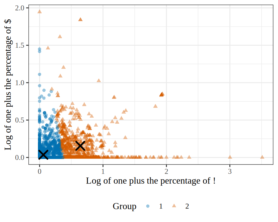
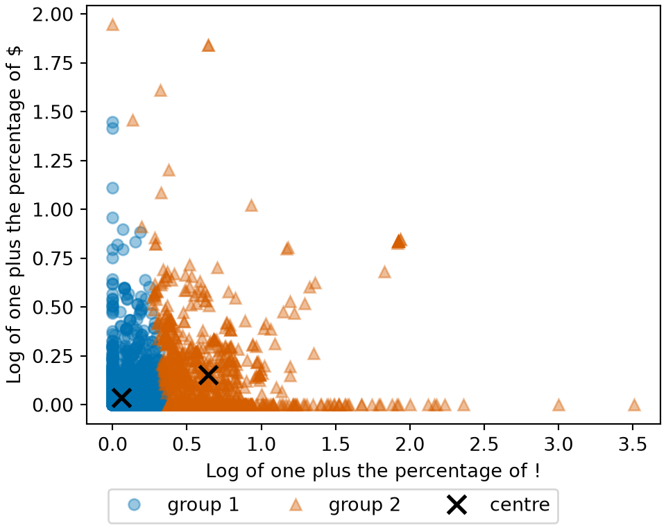
Figure 7: The two groups that \(k\)-means found in Example 11, with the two group centers marked by black crosses. The method never saw the class of the messages.
(a)
Scatter plot of the Spambase messages by the log of one plus the percentage of exclamation marks on the horizontal axis and the log of one plus the percentage of dollar signs on the vertical axis. Most points crowd near the origin. Points in group 1 are drawn as blue circles and points in group 2 as vermilion triangles, with group 2 covering the messages with a larger percentage of exclamation marks and group 1 those with few, including a few with many dollar signs. Black crosses mark the two group centres, one near the origin and one further up and to the right.
(b)
Scatter plot of the Spambase messages by the log of one plus the percentage of exclamation marks on the horizontal axis and the log of one plus the percentage of dollar signs on the vertical axis. Most points crowd near the origin. Points in group 1 are drawn as blue circles and points in group 2 as vermilion triangles, with group 2 covering the messages with a larger percentage of exclamation marks and group 1 those with few, including a few with many dollar signs. Black crosses mark the two group centres, one near the origin and one further up and to the right.
ReadingRead

GeeksforGeeks explains \(k\)-means clustering [22].

ExrExercise 12 (Let the computer find groups)

Exercise 12 (Let the computer find groups) Here are the cars of the Auto data again, plotted by weight and mpg, this time with no labels. First, by eye: how many groups do you see, and where are they?

Show code
viewof kmShow = Inputs.radio(["no groups", "k-means groups"], {value: "no groups", label: "show"})
viewof kmK = Inputs.range([2, 5], {width: 360, value: 2, step: 1, label: "k (groups)"})
viewof kmIter = Inputs.range([0, 15], {width: 360, value: 0, step: 1, label: "iterations"})
viewof kmCompare = Inputs.radio(["nothing", "origin", "cylinders"], {value: "nothing", label: "compare with"})
Show code
kmLabels = kmRun(kmK, kmIter).map((j) => `group ${j + 1}`)
Show code
Plot.plot({
  ariaLabel: 'Scatter plot of the Auto cars, mpg against weight. The points are gray until k-means groups are shown, and then each group has its own color.',
  height: 320, width: 760, grid: true,
  x: {label: "weight (lb)"}, y: {label: "mpg"},
  color: {legend: kmShow === "k-means groups", type: "ordinal", scheme: "category10"},
  marks: [Plot.dot(auto, {x: "weight", y: "mpg", r: 3, fillOpacity: 0.8,
                          fill: kmShow === "k-means groups" ? (d, i) => kmLabels[i] : "#777",
                          tip: true, title: "name"})]
})
Show code
{
  if (kmShow !== "k-means groups" || kmCompare === "nothing") return md``;
  const values = Array.from(new Set(auto.map((d) => d[kmCompare]))).sort((a, b) => a - b);
  const groups = Array.from(new Set(kmLabels)).sort();
  const count = (g, v) => auto.filter((d, i) => kmLabels[i] === g && d[kmCompare] === v).length;
  const head = `| ${kmCompare}: | ${values.join(" | ")} |`;
  const rule = `|:--|${values.map(() => "--:").join("|")}|`;
  const rows = groups.map((g) => `| ${g} | ${values.map((v) => count(g, v)).join(" | ")} |`);
  return md`${[head, rule, ...rows].join("\n")}`;
}
Figure 8: k-means on the Auto cars’ weight and mpg, step by step, with its groups compared against origin or cylinders.

In origin, 1 is American, 2 is European and 3 is Japanese.

Solution 12. By eye, most people see two groups: light cars with high mpg, and heavy cars with low mpg.

ExrExercise 13 (Let the computer find groups (part 2))

Exercise 13 (Let the computer find groups (part 2)) Use the setup of Exercise 12.

Then let k-means (Definition 18) look. Choose \(k\), and step through the iterations. At what iteration does it stop changing?

Solution 13. K-means with \(k = 2\) agrees and stops changing after one iteration. It finds 217 light cars, averaging 2335 lb and 29 mpg, and 175 heavy ones, averaging 3774 lb and 17 mpg.Larger \(k\) also takes longer to stop changing: \(k = 3\) is still changing until its ninth iteration.

ExrExercise 14 (Let the computer find groups (part 3))

Exercise 14 (Let the computer find groups (part 3)) Use the setup of Exercise 12.

Then compare its groups with origin and with cylinders. Which one do the groups match better?

Solution 14. The groups match cylinders much better than origin. The heavy group holds all 103 eight-cylinder cars, and the light group holds 194 of the 199 four-cylinder cars. By origin, the heavy group is almost all American (163 of 175), but the light group mixes all three: 82 American, 58 European and 77 Japanese cars. European and Japanese cars have much the same weights and mpg, so no grouping of these two variables could separate them.

The mismatch with origin shows a limitation of unsupervised learning. The algorithm finds structure in the data, and that structure need not match the label we care about. The algorithm always returns \(k\) groups, even if the data hold fewer, so choosing \(k\) is itself a question. Unsupervised Learning returns to k-means, and to that question.

2.2 Regression and classification

ExrExercise 15 (How do outputs differ?)

Exercise 15 (How do outputs differ?) Supervised problems are named for their output. Compare two supervised problems: predicting a house’s price, and labeling a message spam or email. How does the output \(y\) differ between them?

Solution 15. A house’s price is a number, and a message’s label is one of two categories.

DefDefinition 19 (Regression)

Definition 19 (Regression) A supervised problem (Definition 13) is a regression problem when the output \(y\) is a quantity, such as a price or a temperature, or a vector of quantities [23].

DefDefinition 20 (Classification)

Definition 20 (Classification) A supervised problem (Definition 13) is a classification problem when \(y\) is one of a fixed set of categories, such as spam or email [24].

With two classes the problem is binary classification; with more, it is multi-class classification.

Other names: the categories are also called classes.

ExmExample 12 (Predicting mpg versus predicting spam)

Example 12 (Predicting mpg versus predicting spam) Look at the output \(y\) of two problems from this page: a car’s mpg in the Auto data [10], and a message’s Class in the Spambase data [7].

import pandas as pd

auto_rc = pd.read_csv("data/auto.csv")
spam_rc = pd.read_csv("data/spambase.csv")

# mpg takes many different values along a scale: a quantity.
print(auto_rc["mpg"].describe().round(1))
count    392.0
mean      23.4
std        7.8
min        9.0
25%       17.0
50%       22.8
75%       29.0
max       46.6
Name: mpg, dtype: float64
# Class takes just two values, standing for spam and email: a category.
print(spam_rc["Class"].value_counts())
Class
0    2788
1    1813
Name: count, dtype: int64
auto_rc <- read.csv("data/auto.csv")
spam_rc <- read.csv("data/spambase.csv", check.names = FALSE)

# mpg takes many different values along a scale: a quantity.
summary(auto_rc$mpg)
   Min. 1st Qu.  Median    Mean 3rd Qu.    Max. 
   9.00   17.00   22.75   23.45   29.00   46.60 
# Class takes just two values, standing for spam and email: a category.
table(spam_rc$Class)

   0    1 
2788 1813 

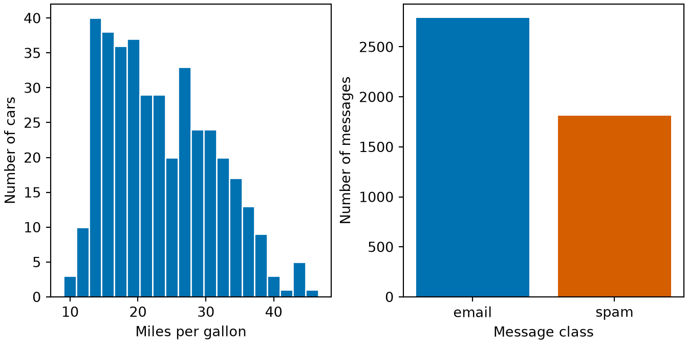
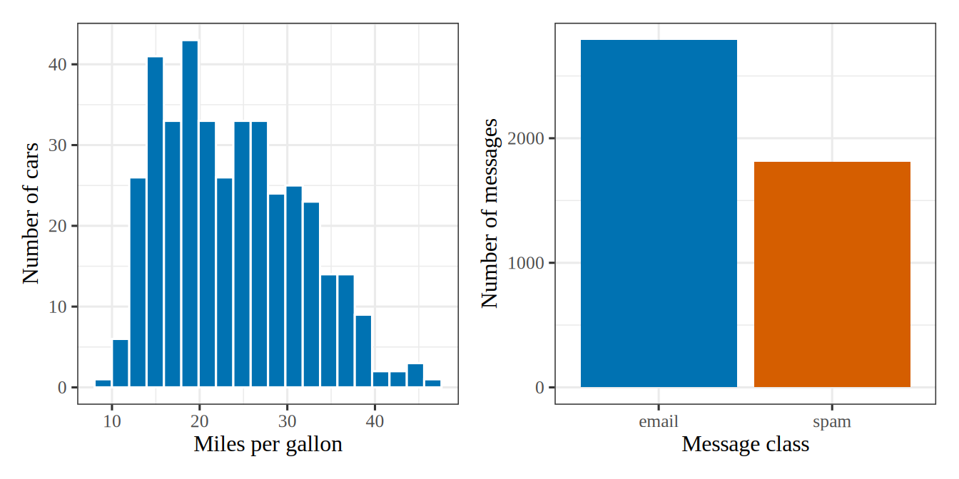
Predicting mpg, which takes 127 distinct values between 9 and 46.6, is a regression problem (Definition 19). Predicting Class, which takes 2 values, is a classification problem (Definition 20), and a binary one because there are two classes. What decides the kind of problem is the output: predicting a car’s origin, coded 1, 2 or 3 but standing for a country, would be classification too.

Show code
library(ggplot2)
library(patchwork)
rg_mpg <- ggplot(auto_rc, aes(mpg)) +
  geom_histogram(bins = 20, fill = "#0072B2", colour = "white") +
  labs(x = "Miles per gallon", y = "Number of cars")
rg_class <- ggplot(
  data.frame(Class = factor(spam_rc$Class, levels = 0:1, labels = c("email", "spam"))),
  aes(Class, fill = Class)
) +
  geom_bar(show.legend = FALSE) +
  scale_fill_manual(values = c(email = "#0072B2", spam = "#D55E00")) +
  labs(x = "Message class", y = "Number of messages")
rg_mpg + rg_class
Show code
import matplotlib.pyplot as plt

fig, (ax_mpg, ax_class) = plt.subplots(1, 2, figsize=(7, 3.5), layout="constrained")
ax_mpg.hist(auto_rc["mpg"], bins=20, color="#0072B2", edgecolor="white");
ax_mpg.set_xlabel("Miles per gallon");
ax_mpg.set_ylabel("Number of cars");
counts_rg = spam_rc["Class"].value_counts().sort_index()
ax_class.bar(["email", "spam"], counts_rg.to_numpy(), color=["#0072B2", "#D55E00"]);
ax_class.set_xlabel("Message class");
ax_class.set_ylabel("Number of messages");
plt.show()
Figure 9: On the left, the output of a regression takes many values along a scale, such as the mpg of cars; on the right, the output of a classification takes just a few, such as the two Class values of messages (Example 12).
(a)
Two panels side by side. The left panel is a histogram of the miles per gallon of the cars in the Auto data, spread over a scale from about 9 to 47 with most cars between 15 and 30 and a longer tail to the right. The right panel is a bar chart of the Spambase message class with two bars, email, which is the taller at about 2800 messages, and spam, at about 1800.
(b)
Two panels side by side. The left panel is a histogram of the miles per gallon of the cars in the Auto data, spread over a scale from about 9 to 47 with most cars between 15 and 30 and a longer tail to the right. The right panel is a bar chart of the Spambase message class with two bars, email, which is the taller at about 2800 messages, and spam, at about 1800.
ReadingRead

GeeksforGeeks explains classification and regression [25].

The spam filter is a classification problem with two classes. Predicting the log of a prostate-cancer antigen level in the blood from clinical measurements is a regression problem. So is predicting a house’s price from its living area, using 47 houses in Portland, Oregon. Other output types exist, such as a ranking of search results by relevance or a sequence of part-of-speech tags, one for each word of a sentence, but these two are the focus of most of this course.

ExrExercise 16 (Regression or classification?)

Exercise 16 (Regression or classification?) Is predicting mpg from the other Auto data variables a regression or a classification problem?

Solution 16. Predicting mpg is regression, because mpg is a quantity.

ExrExercise 17 (Regression or classification? (part 2))

Exercise 17 (Regression or classification? (part 2)) Use the setup of Exercise 16.

Is predicting origin a regression or a classification problem?

Solution 17. Predicting origin is classification, because origin is one of three categories, even though it is stored as the numbers 1, 2 and 3.

2.3 A first regression model

ExrExercise 18 (What is the simplest rule?)

Exercise 18 (What is the simplest rule?) We want a rule that takes a car’s horsepower and returns a predicted mpg.

What is the simplest shape such a rule can take?

Solution 18. A straight line, \[ \eoutvar = \hcoef{0} + \hcoef{1} \predvar, \] where - \(\predvar\) is a car’s horsepower (horsepower); - \(\eoutvar\) is its predicted mpg; - \(\hcoef{0}\) is the intercept; - \(\hcoef{1}\) is the slope.

ExrExercise 19 (What is the simplest rule? (part 2))

Exercise 19 (What is the simplest rule? (part 2)) Use the setup of Exercise 18.

How many numbers do we have to choose to specify that rule exactly?

Solution 19. Two: \(\hcoef{0}\) and \(\hcoef{1}\). To choose them, we need a way to score a line.

ExrExercise 20 (How could we score a line?)

Exercise 20 (How could we score a line?) The line’s error on each car is \(y - \hat{y}\). Propose one number that scores the line on \(n\) cars, so that a lower score means a better line.

Solution 20. Square each car’s error, so that errors above and below the line both increase its total, and average the squares over the \(n\) cars.

DefDefinition 21 (Sample mean squared error)

Definition 21 (Sample mean squared error) The sample mean squared error (sMSE) of a fitted model on \(n\) examples \((x_1, y_1), \ldots, (x_n, y_n)\) is the average squared error [26], \[ \sMSEt = \frac{1}{n} \sum_{i=1}^{n} (y_i - \hat{y}_i)^2, \] where \(\hat{y}_i\) is the fitted model’s prediction for example \(i\).

RemarkRemark 6 (The sMSE estimates the risk)

Remark 6 (The sMSE estimates the risk). The sMSE is a sample estimate of the expected squared error on new examples, the risk under squared error.

ExmExample 13 (A baseline’s sample mean squared error on Auto)

Example 13 (A baseline’s sample mean squared error on Auto) The simplest rule for predicting mpg in the Auto data [10] ignores the car and always guesses the sample mean mpg. Compute its sMSE, and compare it with the sMSE of a line that uses horsepower:

import numpy as np
import pandas as pd

auto_ms = pd.read_csv("data/auto.csv")
y_ms = auto_ms["mpg"].to_numpy(float)

# Baseline: predict the mean mpg for every car.
mse_base_ms = np.mean((y_ms - y_ms.mean()) ** 2)

# Line: predict from horsepower, with the least squares fit.
slope_ms, intercept_ms = np.polyfit(auto_ms["horsepower"], y_ms, 1)
pred_ms = intercept_ms + slope_ms * auto_ms["horsepower"].to_numpy()
mse_line_ms = np.mean((y_ms - pred_ms) ** 2)

print("baseline sMSE:", round(mse_base_ms, 1))
baseline sMSE: 60.8
print("line sMSE:    ", round(mse_line_ms, 1))
line sMSE:     23.9
auto_ms <- read.csv("data/auto.csv")
y_ms <- auto_ms$mpg

# Baseline: predict the mean mpg for every car.
mse_base_ms <- mean((y_ms - mean(y_ms))^2)

# Line: predict from horsepower, with the least squares fit.
fit_ms <- lm(mpg ~ horsepower, data = auto_ms)
mse_line_ms <- mean((y_ms - fitted(fit_ms))^2)

cat("baseline sMSE:", round(mse_base_ms, 1), "\n")
baseline sMSE: 60.8 
cat("line sMSE:    ", round(mse_line_ms, 1), "\n")
line sMSE:     23.9 

On these 392 cars the baseline’s sMSE (Definition 21) is 60.8, in squared miles per gallon, and the line’s is 23.9. The line’s sMSE cannot be larger, because the baseline is a line with slope 0. The line’s sMSE is smaller by a factor of 2.54.

DefDefinition 22 (Sample root mean squared error)

Definition 22 (Sample root mean squared error) The sample root mean squared error (sRMSE) of a fitted model on \(n\) examples is the square root of its sMSE (Definition 21) [27], \[ \sRMSEt = \sqrt{\sMSEt}. \]

RemarkRemark 7 (The sRMSE has the unit of the outcome)

Remark 7 (The sRMSE has the unit of the outcome). Squaring the errors squares their unit, and the square root returns the sRMSE to the unit of the outcome. The sRMSE ranks fitted models in the same order as the sMSE (Definition 21), because the square root is increasing. We therefore report the sRMSE, and later say more about why.

ExmExample 14 (A baseline’s sample root mean squared error on Auto)

Example 14 (A baseline’s sample root mean squared error on Auto) Take the square root of the two sMSEs from Example 13:

print("baseline sRMSE:", round(np.sqrt(mse_base_ms), 2))
baseline sRMSE: 7.8
print("line sRMSE:    ", round(np.sqrt(mse_line_ms), 2))
line sRMSE:     4.89
rmse_base_ms <- sqrt(mse_base_ms)
rmse_line_ms <- sqrt(mse_line_ms)
cat("baseline sRMSE:", round(rmse_base_ms, 2), "\n")
baseline sRMSE: 7.8 
cat("line sRMSE:    ", round(rmse_line_ms, 2), "\n")
line sRMSE:     4.89 

The baseline’s sRMSE (Definition 22) is 7.80 miles per gallon, the same unit as mpg, and the line’s is 4.89. Using horsepower shrinks the typical error by a factor of 1.59.

VideosWatch

Hutchinson explains a model, training and a loss step by step, Machine Learning Example (21 min) [28].

ReadingRead

GeeksforGeeks explains mean squared error [29].

Squaring makes every error increase the rule’s total, and makes big errors count much more than small ones.

ExrExercise 21 (Score a line by hand)

Exercise 21 (Score a line by hand) Take the line \(\hat{y} = 40 - 0.16x\) and the first three cars in Auto:

Table 1: The first three cars, with horsepower and fuel economy.
car horsepower \(x\) mpg \(y\)
chevrolet chevelle malibu 130 18
buick skylark 320 165 15
plymouth satellite 150 18

For each car, find the prediction \(\hat{y}\) and the error \(y - \hat{y}\). Then find the line’s sMSE (Definition 21) on these three cars, and take its square root to get the sRMSE (Definition 22).

Solution 21.

Table 2: The line’s value, its gap and the gap multiplied by itself for each of the three cars.
car \(\hat{y} = 40 - 0.16x\) error \(y - \hat{y}\) squared
chevrolet chevelle malibu \(40 - 20.8 = 19.2\) \(-1.2\) 1.44
buick skylark 320 \(40 - 26.4 = 13.6\) \(1.4\) 1.96
plymouth satellite \(40 - 24.0 = 16.0\) \(2.0\) 4.00

The average of the squared errors is \[ \frac{1.44 + 1.96 + 4.00}{3} = \frac{7.40}{3} \approx 2.47. \] That average is the line’s sMSE on these three cars (Definition 21). Its square root, \(\sqrt{7.40/3} \approx 1.57\) miles per gallon, is the line’s sRMSE (Definition 22).

ExrExercise 22 (Fit a line yourself)

Exercise 22 (Fit a line yourself) Now score lines on all 392 cars at once. Move the intercept and slope to make the sRMSE (Definition 22) as small as you can. What is the lowest sRMSE you can reach?

Show code
viewof fitB0 = Inputs.range([20, 60], {width: 360, value: 30, step: 0.1, label: "intercept b0"})
viewof fitB1 = Inputs.range([-0.4, 0.1], {width: 360, value: -0.05, step: 0.001, label: "slope b1"})
viewof fitShow = Inputs.checkbox(
  ["least-squares line", "least-squares curve"],
  {label: "also show"}
)
Show code
yourMse = mseOf((x) => fitB0 + fitB1 * x)
Show code
{
  const sign = (b) => (b < 0 ? "\u2212" : "+");
  const ls = fitShow.includes("least-squares line")
    ? ` The least-squares line is mpg = ${lsLine.b0.toFixed(2)} ${sign(lsLine.b1)} ${Math.abs(lsLine.b1).toFixed(4)} \u00d7 horsepower, with sRMSE ${rmseOf((x) => lsLine.b0 + lsLine.b1 * x).toFixed(2)}.`
    : "";
  return md`Your line: mpg = ${fitB0.toFixed(1)} ${sign(fitB1)} ${Math.abs(fitB1).toFixed(3)} \u00d7 horsepower,
with sRMSE **${Math.sqrt(yourMse).toFixed(2)}**.
Predicting the sample mean, ${mpgMean.toFixed(1)}, for every car has sRMSE ${Math.sqrt(meanMse).toFixed(2)}.${ls}`;
}
Show code
Plot.plot({
  ariaLabel: 'Scatter plot of mpg against horsepower for the Auto cars, with a dotted gray line at the average mpg, a red line set by the intercept and slope controls, and optionally the least-squares line and curve.',
  height: 340, width: 560, grid: true,
  x: {label: "horsepower", domain: [40, 235]},
  y: {label: "mpg", domain: [5, 50]},
  marks: [
    Plot.dot(autoFit, {x: "horsepower", y: "mpg", r: 2.5, fill: "#888", fillOpacity: 0.6,
                       tip: true, title: "name"}),
    Plot.ruleY([mpgMean], {stroke: "#aaa", strokeDasharray: "2,3"}),
    Plot.line(hpGrid, {x: (x) => x, y: (x) => fitB0 + fitB1 * x,
                       stroke: "#d62728", strokeWidth: 2.5, clip: true}),
    fitShow.includes("least-squares line")
      ? Plot.line(hpGrid, {x: (x) => x, y: (x) => lsLine.b0 + lsLine.b1 * x,
                           stroke: "#1f77b4", strokeWidth: 2, strokeDasharray: "6,4", clip: true})
      : null,
    fitShow.includes("least-squares curve")
      ? Plot.line(hpGrid, {x: (x) => x, y: (x) => lsQuad[0] + lsQuad[1] * x + lsQuad[2] * x * x,
                           stroke: "#2ca02c", strokeWidth: 2, clip: true})
      : null
  ]
})
Figure 10: A line fit by hand to mpg against horsepower, with its mean squared error beside the least-squares fit’s.

The red line is yours; the dotted gray line is the average mpg.

Solution 22.

ExrExercise 23 (Fit a line yourself (part 2))

Exercise 23 (Fit a line yourself (part 2)) Use the setup of Exercise 22.

How does the lowest sRMSE you reached compare with the sRMSE of ignoring horsepower and predicting the sample mean mpg for every car?

Solution 23.

ExrExercise 24 (Is a straight line the right shape?)

Exercise 24 (Is a straight line the right shape?) Look at where the cars are relative to the least-squares line, at low, middle and high horsepower. Is there a pattern in the errors?

Solution 24. The errors have a pattern. The line predicts too low at both ends, below about 80 and above about 170 horsepower, and too high in the middle, because mpg falls steeply at first and then flattens.

ExrExercise 25 (Is a straight line the right shape? (part 2))

Exercise 25 (Is a straight line the right shape? (part 2)) Use the setup of Exercise 24.

Then tick least-squares curve, which fits \(\hat{y} = \hcoef{0} + \hcoef{1} x + \hcoef{2} x^2\) by least squares. Should we always prefer the model with the lower sRMSE (Definition 22)?

Solution 25.

But a lower sRMSE on the data we fit is not the goal. A curve with enough terms could pass through every car and reach an sRMSE of zero, and still predict the next car badly. Minimizing sRMSE on the data we fit repeats the mistake of trusting the best spam rule’s score on half A. The error that matters is the error on data the rule has not seen, which is generalization, the subject of A First Model and Generalization.

VideosWatch

Abu-Mostafa sorts learning problems into supervised, unsupervised and reinforcement learning in his first Caltech lecture, from 36:04 [8], Lecture 1.

3 Learning a game from self-play

3.1 Scoring a checkers position

A program that plays checkers has to choose a move on every turn. One way to choose is to look at the positions each move could lead to, score each position, and pick the move whose position scores best.

ExrExercise 26 (Describe a checkers position with numbers)

Exercise 26 (Describe a checkers position with numbers) Suppose the program plays Black. List four numbers you could compute from a checkers board that say whether the position is good for Black.

TipHint

Think about what a checkers player counts or looks at before deciding who is ahead.

Solution 26. Four good choices:

  • piece advantage: Black’s pieces minus White’s pieces, with a king counted as more than a man;
  • mobility: the number of squares Black could move a piece to;
  • center control: the number of Black pieces on the eight central squares;
  • advancement: how far Black’s men have moved toward the far row, where they become kings.

The IBM checkers program used all four, from a list of 38 such features plus piece advantage [30], “Term replacement”.

ExrExercise 27 (What does scoring a position take?)

Exercise 27 (What does scoring a position take?) To pick a move, the program scores each position it could reach. What goes into that scoring rule, and what comes out?

Solution 27. A board position goes in, and one number comes out. A bigger number should mean the position is better for Black. So the scoring rule is a function from positions to numbers.

DefDefinition 23 (Evaluation function)

Definition 23 (Evaluation function) An evaluation function \(V\) assigns a number \(V(s)\) to each game position \(s\), with a larger number meaning the position is better for the player it scores [31].

ExmExample 15 (Scoring a position by who has more pieces)

Example 15 (Scoring a position by who has more pieces) Score a position \(s\) from Black’s side with \[ V(s) = \begin{cases} 1 & \text{if Black has more pieces than White,} \\ 0 & \text{if the two sides have the same number of pieces,} \\ -1 & \text{if Black has fewer pieces than White.} \end{cases} \] A position \(s\) where Black has 7 pieces and White has 5 scores \(V(s) = 1\).

ExrExercise 28 (Combine the features into one score)

Exercise 28 (Combine the features into one score) How could the program combine the numbers from Exercise 26 into a single score for a position?

Solution 28. Give each feature a weight, multiply each feature by its weight, and add up the products. A feature that matters more for winning gets a larger weight.

DefDefinition 24 (Linear evaluation function)

Definition 24 (Linear evaluation function) A linear evaluation function is an evaluation function (Definition 23) that is a weighted sum, the dot product of a weight vector with a feature vector (Definition 8) describing the position, \[ V_{w}(s) = \sum_{j=1}^{\ninputvars} w_j x_j(s), \] where \(x_1(s), \ldots, x_{\ninputvars}(s)\) are the features of \(s\), and the numbers \(w_1, \ldots, w_{\ninputvars}\) are its weights.

ExmExample 16 (A two-feature evaluation function)

Example 16 (A two-feature evaluation function) Take two features, \(x_1(s)\), Black’s piece advantage, and \(x_2(s)\), Black’s mobility advantage (the number of squares Black can move a piece to, minus White’s number), with weights \(w_1 = 3\) and \(w_2 = 1\). A position \(s\) where Black is ahead by one piece and can move to 5 more squares than White scores \[ \begin{aligned} V_{w}(s) &= 3 \times 1 + 1 \times 5 \\ &= 8. \end{aligned} \]

The features say what the program looks at. The weights say how much each feature matters, and the program can learn the weights.

ExrExercise 29 (Where can the weights come from?)

Exercise 29 (Where can the weights come from?) Name three ways to choose the weights \(w_1, \ldots, w_{\ninputvars}\) of a linear evaluation function for checkers (Definition 24).

Solution 29.

  1. A person sets them by hand, from experience of the game. No learning happens.
  2. The program learns them from games between expert players, choosing weights whose top-scored move tends to match the move the expert made.
  3. The program learns them from games it plays against itself.
ExrExercise 30 (Where can the weights come from? (part 2))

Exercise 30 (Where can the weights come from? (part 2)) Use the setup of Exercise 29.

Which of your three ways count as machine learning?

Solution 30. Ways 2 and 3 are machine learning: the program’s play improves with experience, and the experience is data, not rules a person wrote down. The IBM checkers program learned its weights by way 3 in 1959 [30]. A 1967 follow-up reported an improved “book learning” procedure, which Samuel judged “much superior to the linear polynomial method” [32], abstract.

3.2 Learning from self-play

Nobody tells a program playing against itself how good a position really is, or which move was correct. Learning from self-play is a kind of reinforcement learning (Definition 16), and the program has to make its own targets.

ExrExercise 31 (Score a position by looking ahead)

Exercise 31 (Score a position by looking ahead) The evaluation function scores a position from its features alone. How could the program use the evaluation function to get a more reliable score for a position \(s\), by looking several moves ahead of \(s\)?

Solution 31. Look at every position the game could reach from \(s\) within a few moves, and score each of those positions with the evaluation function. Then work backwards, assuming each player picks the move that is best for that player.

DefDefinition 25 (Backed-up score)

Definition 25 (Backed-up score) The backed-up score of a position \(s\) looks several moves ahead: it applies the evaluation function to every position reachable from \(s\) within a fixed number of moves, then assumes each side picks the move best for itself, working back one move at a time until it reaches \(s\) [33].

ExmExample 17 (A two-move backed-up score)

Example 17 (A two-move backed-up score) In position \(s\), Black is to move and has two moves, A and B. White then has two replies to each. The evaluation function scores the four resulting positions for Black:

Table 3: The four resulting positions of the two-move game, with the value of each for Black.
Black’s move White’s reply score for Black
A A1 \(5\)
A A2 \(1\)
B B1 \(3\)
B B2 \(2\)

White picks the reply that is worst for Black, so move A is worth \(\min(5, 1) = 1\) and move B is worth \(\min(3, 2) = 2\). Black picks the better of the two moves, so the backed-up score of \(s\) is \(\max(1, 2) = 2\).

ExrExercise 32 (A target without labels)

Exercise 32 (A target without labels) The program has two ways to score a position \(s\): the evaluation function \(V_{w}(s)\) (Definition 24), and the backed-up score of \(s\) (Definition 25). Which of the two should the program trust more?

Solution 32. The backed-up score is more trustworthy.

ExrExercise 33 (A target without labels (part 2))

Exercise 33 (A target without labels (part 2)) Use the setup of Exercise 32.

Why should the program trust that one more?

Solution 33. The backed-up score has seen more of the game: it scores positions several moves further on, where more of the outcome is already settled.

ExrExercise 34 (A target without labels (part 3))

Exercise 34 (A target without labels (part 3)) Use the setup of Exercise 32.

How could the program use the one it trusts more to improve the weights \(w\)?

Solution 34. So the program can treat the backed-up score as the target, and change the weights until \(V_{w}(s)\) comes closer to it.

we are attempting to make the score, calculated for the current board position, look like that calculated for the terminal board position of the chain of moves which most probably will occur during actual play.

[30], “Polynomial modification procedure”

ExrExercise 35 (Score a position and find the gap)

Exercise 35 (Score a position and find the gap) Use the two-feature evaluation function of Example 16, with a new position \(s\) and these values:

Table 4: The symbols, meanings and values for the position.
symbol meaning value
\(x_1(s)\) Black’s piece advantage in \(s\) \(2\)
\(x_2(s)\) Black’s mobility advantage in \(s\) \(-1\)
\(w_1, w_2\) current weights \(1, 1\)
\(t\) backed-up score of \(s\) (Definition 25) \(3\)

Find the score \(V_{w}(s)\) and the gap \(\delta = t - V_{w}(s)\) between the target and the score.

Solution 35. \[ \begin{aligned} V_{w}(s) &= w_1 x_1(s) + w_2 x_2(s) && \text{(definition of } V_w\text{)} \\ &= 1 \times 2 + 1 \times (-1) && \text{(substitute the values)} \\ &= 1, \\ \delta &= t - V_{w}(s) && \text{(definition of } \delta\text{)} \\ &= 3 - 1 && \text{(substitute the values)} \\ &= 2. \end{aligned} \]

The score is too low by 2.

ExrExercise 36 (Change the weights slightly)

Exercise 36 (Change the weights slightly) One rule for changing the weights is \[ w_j \leftarrow w_j + \eta \, \delta \, x_j(s), \] where the step size \(\eta\) controls how far each weight moves. Use \(\eta = 0.1\) and your \(\delta\) from Exercise 35 to find the new weights \(w_1\) and \(w_2\).

Solution 36. \[ \begin{aligned} w_1 &\leftarrow w_1 + \eta \, \delta \, x_1(s) && \text{(the update rule, } j = 1\text{)} \\ &= 1 + 0.1 \times 2 \times 2 && \text{(substitute the values)} \\ &= 1.4, \\ w_2 &\leftarrow w_2 + \eta \, \delta \, x_2(s) && \text{(the update rule, } j = 2\text{)} \\ &= 1 + 0.1 \times 2 \times (-1) && \text{(substitute the values)} \\ &= 0.8. \end{aligned} \]

The score was too low (\(\delta > 0\)), so the weight on the feature that raised the score (\(x_1 > 0\)) grew, and the weight on the feature that lowered the score (\(x_2 < 0\)) shrank.

ExrExercise 37 (Check the new score)

Exercise 37 (Check the new score) Find the new score \(V_{w}(s)\) with the new weights from Exercise 36.

Solution 37. \[ \begin{aligned} V_{w}(s) &= w_1 x_1(s) + w_2 x_2(s) && \text{(definition of } V_w\text{)} \\ &= 1.4 \times 2 + 0.8 \times (-1) && \text{(substitute the new weights)} \\ &= 2.8 - 0.8 && \text{(multiply)} \\ &= 2.0. \end{aligned} \]

ExrExercise 38 (Check the new score (part 2))

Exercise 38 (Check the new score (part 2)) Use the setup of Exercise 37.

Did the score move toward the target \(t = 3\)?

Solution 38. The new score, 2.0, is closer to \(t = 3\) than the old score of 1.

The IBM program followed the same principle with a different rule. It kept, for each feature, a correlation between the sign of that feature’s contribution to the score and the sign of \(\delta\), and set the weights to powers of 2 in proportion to those correlations. It also swapped the feature with the weakest correlation for one from a reserve list, about once every eight moves [30], “Polynomial modification procedure” and “Term replacement”. The rule in Exercise 36 is a later, simpler one.

ExrExercise 39 (Remember positions you have scored)

Exercise 39 (Remember positions you have scored) Suppose the program looks 3 moves ahead, and it saves every position it meets in play, together with that position’s backed-up score (Definition 25). The 3-move lookahead in a later game reaches one of the saved positions. How far ahead does the saved score effectively look?

Solution 39. The saved score already looks 3 moves past the saved position, and the saved position is 3 moves past the current one, so the score in use looks \(3 + 3 = 6\) moves ahead. The memory grows with every game, and the effective lookahead grows with the memory.

The IBM program saved over 53,000 positions this way. It learned to play good openings and endgames, though its midgame play barely improved [30], “Rote-learning tests”.

4 Going further

The rest of this page is optional: we do it in class if there is time, and otherwise it is here for you to work through on your own.

4.1 More on the spam data

ExrExercise 40 (Look at the spam data)

Exercise 40 (Look at the spam data) The spam data are the Spambase set, collected at Hewlett-Packard Labs and published in the UCI Machine Learning Repository [7]. The same 4601 messages also ship as spam in R’s kernlab package [34], and Python’s ucimlrepo package downloads them from UCI. These notes keep a copy of the file, with UCI’s column names, at data/spambase.csv, so each spam exercise in this section that loads the data reads the same file.

Load it.

Solution 40.

Show code
import pandas as pd

spam = pd.read_csv("data/spambase.csv")
Show code
spam <- read.csv("data/spambase.csv", check.names = FALSE)
ExrExercise 41 (Look at the spam data (part 2))

Exercise 41 (Look at the spam data (part 2)) Use the setup of Exercise 40.

Look at the george, you, free and hp columns.

Solution 41.

Show code
print(spam[["word_freq_george", "word_freq_you",
            "word_freq_free", "word_freq_hp"]].head())
   word_freq_george  word_freq_you  word_freq_free  word_freq_hp
0               0.0           1.93            0.32           0.0
1               0.0           3.47            0.14           0.0
2               0.0           1.36            0.06           0.0
3               0.0           3.18            0.31           0.0
4               0.0           3.18            0.31           0.0
Show code
spam |>
  dplyr::select(word_freq_george, word_freq_you,
                word_freq_free, word_freq_hp) |>
  str()
'data.frame':   4601 obs. of  4 variables:
 $ word_freq_george: num  0 0 0 0 0 0 0 0 0 0 ...
 $ word_freq_you   : num  1.93 3.47 1.36 3.18 3.18 0 3.85 0 1.23 1.67 ...
 $ word_freq_free  : num  0.32 0.14 0.06 0.31 0.31 0 0.96 0 0 0 ...
 $ word_freq_hp    : num  0 0 0 0 0 0 0 0 0 0 ...

Most entries are 0: in any one message, most of the 57 words never appear.

ExrExercise 42 (Look at the spam data (part 3))

Exercise 42 (Look at the spam data (part 3)) Use the setup of Exercise 40.

Count how many messages are spam.

Solution 42.

Show code
print(spam["Class"].value_counts())
Class
0    2788
1    1813
Name: count, dtype: int64
Show code
table(spam$Class)

   0    1 
2788 1813 
Show code
n_msg <- nrow(spam)
n_spam <- sum(spam$Class == 1)
n_email <- sum(spam$Class == 0)

There are 4601 messages: 1813 spam and 2788 email. The file codes spam as 1 and email as 0.

ExrExercise 43 (Read the file with R’s defaults)

Exercise 43 (Read the file with R’s defaults) UCI names six of Spambase’s columns after punctuation marks: char_freq_;, char_freq_( and so on. Read data/spambase.csv into R with read.csv() and no other arguments, and print the names of columns 49 to 54.

Solution 43.

default <- read.csv("data/spambase.csv")
names(default)[49:54]
[1] "char_freq_."   "char_freq_..1" "char_freq_..2" "char_freq_..3"
[5] "char_freq_..4" "char_freq_..5"
ExrExercise 44 (Read the file with R’s defaults (part 2))

Exercise 44 (Read the file with R’s defaults (part 2)) Use the setup of Exercise 43.

What happened to them?

Solution 44. Six names changed: ;, (, [, !, $ and # cannot appear in an R name, so each became ., and the six results were made unique by appending .1, .2 and so on.

ExrExercise 45 (Read the file with R’s defaults (part 3))

Exercise 45 (Read the file with R’s defaults (part 3)) Use the setup of Exercise 43.

Why did that happen to them?

Solution 45. By default read.csv passes every column name through make.names(), which turns anything that is not a legal R name into one.

ExrExercise 46 (Read the file with R’s defaults (part 4))

Exercise 46 (Read the file with R’s defaults (part 4)) Use the setup of Exercise 43.

How do you keep the names as they are in the file?

Solution 46.

kept <- read.csv("data/spambase.csv", check.names = FALSE)
names(kept)[49:54]
[1] "char_freq_;" "char_freq_(" "char_freq_[" "char_freq_!" "char_freq_$"
[6] "char_freq_#"

check.names = FALSE keeps the file’s names, which must then be quoted with backticks in $ access: spam$`char_freq_(`.

Python’s pandas.read_csv keeps them as they are, and they are used as strings in either case: spam["char_freq_!"].

ExrExercise 47 (Look at four messages)

Exercise 47 (Look at four messages) The table of spam and email averages gives the average message in each group. Select the same five columns for the first two messages in the file, and for the first two real messages that contain both george and hp.

Solution 47. Python counts rows from 0 and R from 1, so the same four messages are [0, 1, 1818, 1823] in one and c(1, 2, 1819, 1824) in the other.

Show code
import pandas as pd

spam = pd.read_csv("data/spambase.csv")
cols = ["word_freq_george", "word_freq_you", "word_freq_free",
        "char_freq_!", "word_freq_hp", "Class"]
print(spam.loc[[0, 1, 1818, 1823], cols].to_string())
      word_freq_george  word_freq_you  word_freq_free  char_freq_!  word_freq_hp  Class
0                 0.00           1.93            0.32        0.778          0.00      1
1                 0.00           3.47            0.14        0.372          0.00      1
1818              2.04           0.00            0.00        0.000          4.08      0
1823              0.24           0.24            0.00        0.149          9.33      0
Show code
spam <- read.csv("data/spambase.csv", check.names = FALSE)
cols <- c("word_freq_george", "word_freq_you", "word_freq_free",
          "char_freq_!", "word_freq_hp", "Class")
spam |>
  dplyr::mutate(id = dplyr::row_number()) |>
  dplyr::filter(id %in% c(1, 2, 1819, 1824)) |>
  dplyr::select(id, dplyr::all_of(cols)) |>
  knitr::kable()
Table 5: Five of the 57 columns, for two spam messages and two real ones.
id word_freq_george word_freq_you word_freq_free char_freq_! word_freq_hp Class
1 0.00 1.93 0.32 0.778 0.00 1
2 0.00 3.47 0.14 0.372 0.00 1
1819 2.04 0.00 0.00 0.000 4.08 0
1824 0.24 0.24 0.00 0.149 9.33 0
ExrExercise 48 (Look at four messages (part 2))

Exercise 48 (Look at four messages (part 2)) Use the setup of Exercise 47.

Does each message look like its group’s average?

Solution 48.

Show code
you_spam_avg <- mean(spam$word_freq_you[spam$Class == 1])

Each message does look like its group. Neither spam message contains george or hp at all, and both real ones contain both.

An average is not a guarantee, though. Message 1 is spam with you at 1.93, below the spam average of 2.26 and well below message 2’s 3.47. A rule built on one column will misclassify messages that a rule built on several would classify correctly.

ExrExercise 49 (Check the order of the rows)

Exercise 49 (Check the order of the rows) Is the file shuffled? Look at the Class column from top to bottom and say how it is arranged.

Solution 49. Count the runs of a constant label, from the top of the file down:

Show code
import pandas as pd

spam = pd.read_csv("data/spambase.csv")
print(spam["Class"].ne(spam["Class"].shift()).sum())
2
Show code
print(spam["Class"].head(3).tolist(), spam["Class"].tail(3).tolist())
[1, 1, 1] [0, 0, 0]
Show code
spam <- read.csv("data/spambase.csv", check.names = FALSE)
rle(spam$Class)
Run Length Encoding
  lengths: int [1:2] 1813 2788
  values : int [1:2] 1 0
Show code
runs <- rle(spam$Class)
n_train <- floor(0.8 * nrow(spam))

There are 2 runs, so the label changes exactly once: all 1813 spam messages come first, then all 2788 real ones.

ExrExercise 50 (Check the order of the rows (part 2))

Exercise 50 (Check the order of the rows (part 2)) Use the setup of Exercise 49.

Why would the order of the rows matter?

Solution 50. So taking the first 80% of the rows, 3680 of them, as a training set would put every spam message in training and leave a test set of email alone. Any split of this file has to shuffle first, so the two halves in the held-out exercise were drawn at random.

ExrExercise 51 (How many rules did the computer try?)

Exercise 51 (How many rules did the computer try?) The best rule search in the exercise on beating the all-email rule tried every %george threshold from 0 to 5 and every %you threshold from 0 to 10, each in steps of 0.05. Count the candidate rules.

Solution 51. From 0 to 5 in steps of 0.05 is \(5 / 0.05 + 1 = 101\) thresholds, and from 0 to 10 is \(10 / 0.05 + 1 = 201\). Every pair is a rule, so the search tried \(101 \times 201 = 20301\) rules, each scored on all 4601 emails. A computer does that in much less than a second; a person does not.

4.2 Statistical learning: a short history

The name statistical learning is recent, but many of its methods are old [10, Ch. 1]:

  • least squares, the first form of linear regression, in the early 1800s;
  • linear discriminant analysis in 1936, and logistic regression in the 1940s;
  • generalized linear models in the early 1970s;
  • classification and regression trees and neural networks in the 1980s, once computers could fit nonlinear models;
  • support vector machines in the 1990s.

Statisticians and computer scientists developed these methods at the same time. The same tools led to data mining, machine learning and bioinformatics, fields whose methods “have common underpinnings but are often expressed with different terminology” [5], back cover.

VideosWatch

The Data Science Learning Community’s book clubs discuss An Introduction to Statistical Learning, Chapter 1, in recorded meetings:

4.3 Loading the Auto data yourself

ExrExercise 52 (Load the data yourself)

Exercise 52 (Load the data yourself) The Auto data are available as data/auto.csv; the note on the Auto data says where that file comes from. In either language, load the file and report how many rows and columns it has.

Solution 52.

import pandas as pd

# ISLP's load_data("Auto") reads this same file,
# with each car's name as the row index.
Auto = pd.read_csv("data/auto.csv", index_col="name")
print(Auto.shape)
(392, 8)
# The ISLR2 package holds the same data frame, as `Auto`.
Auto <- read.csv("data/auto.csv", stringsAsFactors = TRUE)
str(Auto)
'data.frame':   392 obs. of  9 variables:
 $ mpg         : num  18 15 18 16 17 15 14 14 14 15 ...
 $ cylinders   : int  8 8 8 8 8 8 8 8 8 8 ...
 $ displacement: num  307 350 318 304 302 429 454 440 455 390 ...
 $ horsepower  : int  130 165 150 150 140 198 220 215 225 190 ...
 $ weight      : int  3504 3693 3436 3433 3449 4341 4354 4312 4425 3850 ...
 $ acceleration: num  12 11.5 11 12 10.5 10 9 8.5 10 8.5 ...
 $ year        : int  70 70 70 70 70 70 70 70 70 70 ...
 $ origin      : int  1 1 1 1 1 1 1 1 1 1 ...
 $ name        : Factor w/ 301 levels "amc ambassador brougham",..: 49 36 230 14 160 141 54 222 240 2 ...

Both find 392 cars. Python reports 8 columns, because the code makes each car’s name the row index, as ISLP does; R reports 9, with name as an ordinary column.

ExrExercise 53 (Summarize three variables)

Exercise 53 (Summarize three variables) Now summarize mpg, horsepower and weight. What is the range of each, and the mean of mpg?

Solution 53.

import pandas as pd

Auto = pd.read_csv("data/auto.csv", index_col="name")
print(Auto[["mpg", "horsepower", "weight"]].describe())
              mpg  horsepower       weight
count  392.000000  392.000000   392.000000
mean    23.445918  104.469388  2977.584184
std      7.805007   38.491160   849.402560
min      9.000000   46.000000  1613.000000
25%     17.000000   75.000000  2225.250000
50%     22.750000   93.500000  2803.500000
75%     29.000000  126.000000  3614.750000
max     46.600000  230.000000  5140.000000
Show code
Auto <- read.csv("data/auto.csv", stringsAsFactors = TRUE)
Auto |>
  dplyr::select(mpg, horsepower, weight) |>
  gtsummary::tbl_summary(
    type = gtsummary::all_continuous() ~ "continuous2",
    statistic = gtsummary::all_continuous() ~
      c("{mean} ({sd})", "{min}, {max}"),
    digits = gtsummary::all_continuous() ~ 1
  ) |>
  gtsummary::as_kable()
Characteristic N = 392
mpg
Mean (SD) 23.4 (7.8)
Min, Max 9.0, 46.6
horsepower
Mean (SD) 104.5 (38.5)
Min, Max 46.0, 230.0
weight
Mean (SD) 2,977.6 (849.4)
Min, Max 1,613.0, 5,140.0

mpg runs from 9 to 46.6, with a mean of 23.4; horsepower from 46 to 230; and weight from 1613 to 5140 pounds.

The chapter 2 lab goes further, in Python (Ch02-statlearn-lab.ipynb in the ISLP labs repository) and in R (the chapter 2 files on the book’s R resources page).

4.4 Sorting learning problems

ExrExercise 54 (Supervised or unsupervised?)

Exercise 54 (Supervised or unsupervised?) For each task, decide whether it is supervised or unsupervised.

Recognize which digit, 0 to 9, a handwritten image shows.

Solution 54. Supervised: each image comes with its digit.

ExrExercise 55 (Supervised or unsupervised? (part 2))

Exercise 55 (Supervised or unsupervised? (part 2)) Use the setup of Exercise 54.

Predict tomorrow’s high temperature in Bellingham.

Solution 55. Supervised: past days come with their recorded highs.

ExrExercise 56 (Supervised or unsupervised? (part 3))

Exercise 56 (Supervised or unsupervised? (part 3)) Use the setup of Exercise 54.

Group news articles by topic, with no topics given in advance.

Solution 56. Unsupervised (clustering): no topics are given.

ExrExercise 57 (Supervised or unsupervised? (part 4))

Exercise 57 (Supervised or unsupervised? (part 4)) Use the setup of Exercise 54.

Predict a house’s sale price from its size and location.

Solution 57. Supervised: past sales come with their prices.

ExrExercise 58 (Supervised or unsupervised? (part 5))

Exercise 58 (Supervised or unsupervised? (part 5)) Use the setup of Exercise 54.

Decide whether a credit-card transaction is fraudulent, given past transactions marked as fraud or not.

Solution 58. Supervised: past transactions are marked as fraud or not.

The fraud task can also be an unsupervised problem. A detector could flag transactions unlike the rest even with no labels marking past fraud. That version of the task is called anomaly detection. The same goal can lead to different problems depending on what data exist.

ExrExercise 59 (Supervised or unsupervised? (part 6))

Exercise 59 (Supervised or unsupervised? (part 6)) Use the setup of Exercise 54.

Find groups of customers who shop in similar ways.

Solution 59. Unsupervised (clustering): no groups are given.

ExrExercise 60 (Regression or classification, again)

Exercise 60 (Regression or classification, again) For each supervised task in Exercise 54, decide whether it is regression or classification.

Solution 60.

4.5 Asking questions of data

ExrExercise 61 (Asking questions of data)

Exercise 61 (Asking questions of data) Machine learning starts with a question that data can help answer. A transit agency records card taps at stations, with the time, the line and the weather that day. What patterns might exist in these data?

Solution 61. Many answers work. Some examples:

Public transit: the traffic at a station may depend on the time, the line and the weather, and the traffic at some stations may rise and fall together.

ExrExercise 62 (Asking questions of data (part 2))

Exercise 62 (Asking questions of data (part 2)) What would you want a model to predict from the transit data of Exercise 61?

Solution 62. Public transit: predict how many people will tap in at a station during the next hour from the time, the line and the weather.

ExrExercise 63 (Asking questions of data (part 3))

Exercise 63 (Asking questions of data (part 3)) Would the model of Exercise 62 be supervised or unsupervised?

Solution 63. Public transit: predicting the number of taps is supervised regression, and finding groups of stations whose traffic rises and falls together is unsupervised.

ExrExercise 64 (Asking questions of data (part 4))

Exercise 64 (Asking questions of data (part 4)) A farm records soil samples, planting dates, rainfall and harvest weights for many fields. What patterns might exist in these data?

Solution 64. Farming: a field’s harvest weight may depend on its soil, planting date and rainfall, and fields planted late with little rain may form a group.

ExrExercise 65 (Asking questions of data (part 5))

Exercise 65 (Asking questions of data (part 5)) What would you want a model to predict from the farming data of Exercise 64?

Solution 65. Farming: predict a field’s harvest weight from its soil, planting date and rainfall.

ExrExercise 66 (Asking questions of data (part 6))

Exercise 66 (Asking questions of data (part 6)) Would the model of Exercise 65 be supervised or unsupervised?

Solution 66. Farming: predicting the harvest weight is supervised regression, and flagging fields that were planted late and got little rain is unsupervised grouping.

ExrExercise 67 (Asking questions of data (part 7))

Exercise 67 (Asking questions of data (part 7)) A public library records each loan, with the book’s subject and the borrower’s earlier loans. What patterns might exist in these data?

Solution 67. A public library: borrowers who read one subject may borrow more books on it, and some borrowers may read alike.

ExrExercise 68 (Asking questions of data (part 8))

Exercise 68 (Asking questions of data (part 8)) What would you want a model to predict from the library data of Exercise 67?

Solution 68. A public library: predict whether a borrower will take out a second book from the same subject.

ExrExercise 69 (Asking questions of data (part 9))

Exercise 69 (Asking questions of data (part 9)) Would the model of Exercise 68 be supervised or unsupervised?

Solution 69. A public library: predicting whether a borrower takes a second book is supervised classification, and grouping borrowers by what they read is unsupervised.

ExrExercise 70 (Your own problem)

Exercise 70 (Your own problem) Brainstorm one use of machine learning not mentioned in this lecture, and name its input features and its output.

Solution 70. Answers will vary; we will share a few and sort them together, as supervised or unsupervised. For a supervised one, check that its output is something you could have recorded for past examples, since the model learns from those recorded outputs.

Definitions on this page

References

[1]
Wikipedia contributors, “Feature (machine learning) — Wikipedia, the free encyclopedia.” 2026. Available: https://en.wikipedia.org/wiki/Feature_(machine_learning)
[2]
Wikipedia contributors, “Scientific modelling — Wikipedia, the free encyclopedia.” 2026. Available: https://en.wikipedia.org/wiki/Scientific_modelling
[3]
Wikipedia contributors, “Model — Wikipedia, the free encyclopedia.” 2026. Available: https://en.wikipedia.org/wiki/Model
[4]
G. E. P. Box, “Robustness in the strategy of scientific model building,” in Robustness in statistics, R. L. Launer and G. N. Wilkinson, Eds., Academic Press, 1979, pp. 201–236. doi: 10.1016/B978-0-12-438150-6.50018-2.
[5]
T. Hastie, R. Tibshirani, and J. Friedman, The elements of statistical learning: Data mining, inference, and prediction, 2nd ed. Springer, 2009. Available: https://hastie.su.domains/ElemStatLearn/
[6]
K. P. Murphy, Machine learning: A probabilistic perspective. in Adaptive computation and machine learning. MIT Press, 2012.
[7]
M. Hopkins, E. Reeber, G. Forman, and J. Suermondt, “Spambase.” UCI Machine Learning Repository, 1999. doi: 10.24432/C53G6X.
[8]
Y. S. Abu-Mostafa, “Learning from data: CS 156 lectures.” Caltech, lecture videos on YouTube, 2012. Available: https://www.youtube.com/playlist?list=PLD63A284B7615313A
[9]
K. Weinberger, “CS4780: Machine learning for intelligent systems, spring 2017.” Cornell University, lecture videos on YouTube, 2017. Available: https://www.youtube.com/playlist?list=PLl8OlHZGYOQ7bkVbuRthEsaLr7bONzbXS
[10]
G. James, D. Witten, T. Hastie, and R. Tibshirani, An introduction to statistical learning with applications in R, 2nd ed. Springer, 2021. Available: https://www.statlearning.com/
[11]
G. James, D. Witten, T. Hastie, R. Tibshirani, and J. Taylor, An introduction to statistical learning: With applications in Python. Springer, 2023. doi: 10.1007/978-3-031-38747-0.
[12]
Wikipedia contributors, “Supervised learning — Wikipedia, the free encyclopedia.” 2026. Available: https://en.wikipedia.org/wiki/Supervised_learning
[13]
Wikipedia contributors, “Unsupervised learning — Wikipedia, the free encyclopedia.” 2026. Available: https://en.wikipedia.org/wiki/Unsupervised_learning
[14]
T. Hastie, R. Tibshirani, and J. Taylor, “Statistical learning with python.” Stanford Online, lecture videos on YouTube, 2023. Available: https://www.youtube.com/playlist?list=PLoROMvodv4rPP6braWoRt5UCXYZ71GZIQ
[15]
GeeksforGeeks, “Supervised and unsupervised learning.” GeeksforGeeks, tutorial article, 2025. Available: https://www.geeksforgeeks.org/machine-learning/supervised-unsupervised-learning/
[16]
Wikipedia contributors, “Weak supervision — Wikipedia, the free encyclopedia.” 2026. Available: https://en.wikipedia.org/wiki/Weak_supervision
[17]
Wikipedia contributors, “Reinforcement learning — Wikipedia, the free encyclopedia.” 2026. Available: https://en.wikipedia.org/wiki/Reinforcement_learning
[18]
GeeksforGeeks, “Semi-supervised learning in ML.” GeeksforGeeks, tutorial article, 2026. Available: https://www.geeksforgeeks.org/machine-learning/ml-semi-supervised-learning/
[19]
GeeksforGeeks, “Reinforcement learning.” GeeksforGeeks, tutorial article, 2026. Available: https://www.geeksforgeeks.org/machine-learning/what-is-reinforcement-learning/
[20]
Wikipedia contributors, “Cluster analysis — Wikipedia, the free encyclopedia.” 2026. Available: https://en.wikipedia.org/wiki/Cluster_analysis
[21]
Wikipedia contributors, “K-means clustering — Wikipedia, the free encyclopedia.” 2026. Available: https://en.wikipedia.org/wiki/K-means_clustering
[22]
GeeksforGeeks, “K means clustering – introduction.” GeeksforGeeks, tutorial article, 2026. Available: https://www.geeksforgeeks.org/machine-learning/k-means-clustering-introduction/
[23]
Wikipedia contributors, “Regression analysis — Wikipedia, the free encyclopedia.” 2026. Available: https://en.wikipedia.org/wiki/Regression_analysis
[24]
Wikipedia contributors, “Statistical classification — Wikipedia, the free encyclopedia.” 2026. Available: https://en.wikipedia.org/wiki/Statistical_classification
[25]
GeeksforGeeks, “Classification vs regression in machine learning.” GeeksforGeeks, tutorial article, 2025. Available: https://www.geeksforgeeks.org/machine-learning/ml-classification-vs-regression/
[26]
Wikipedia contributors, “Mean squared error — Wikipedia, the free encyclopedia.” 2026. Available: https://en.wikipedia.org/wiki/Mean_squared_error
[27]
Wikipedia contributors, “Root-mean-square deviation — Wikipedia, the free encyclopedia.” 2026. Available: https://en.wikipedia.org/wiki/Root-mean-square_deviation
[28]
B. Hutchinson, “DATA 471/571 (machine learning) and CSCI 481/581 (deep learning) video lectures.” Western Washington University. Accessed: Sep. 28, 2026. [Online]. Available: https://facultyweb.cs.wwu.edu/~hutchib2/video_lectures/data371/
[29]
GeeksforGeeks, “Mean squared error.” GeeksforGeeks, tutorial article, 2026. Available: https://www.geeksforgeeks.org/maths/mean-squared-error/
[30]
A. L. Samuel, “Some studies in machine learning using the game of checkers,” IBM Journal of Research and Development, vol. 3, no. 3, pp. 210–229, 1959, doi: 10.1147/rd.33.0210.
[31]
Wikipedia contributors, “Evaluation function — Wikipedia, the free encyclopedia.” 2026. Available: https://en.wikipedia.org/wiki/Evaluation_function
[32]
A. L. Samuel, “Some studies in machine learning using the game of checkers. II—recent progress,” IBM Journal of Research and Development, vol. 11, no. 6, pp. 601–617, 1967, doi: 10.1147/rd.116.0601.
[33]
Wikipedia contributors, “Minimax — Wikipedia, the free encyclopedia.” 2026. Available: https://en.wikipedia.org/wiki/Minimax
[34]
A. Karatzoglou, A. Smola, K. Hornik, and A. Zeileis, “kernlab – an S4 package for kernel methods in R,” Journal of Statistical Software, vol. 11, no. 9, pp. 1–20, 2004, doi: 10.18637/jss.v011.i09.
[35]
Data Science Learning Community, “Introduction to statistical learning using R (islr06).” Book club meeting recordings on YouTube, 2023. Available: https://www.youtube.com/playlist?list=PL3x6DOfs2NGjlhpKMiWsDcKL2nngwXROq
[36]
Data Science Learning Community, “Introduction to statistical learning using Python (islp03).” Book club meeting recordings on YouTube, 2025. Available: https://www.youtube.com/playlist?list=PL3x6DOfs2NGgbSNh0UG87rrM-z5LiKLZp
Back to top