Each solution shows the code in Python, in R as the book’s lab writes it, and in R with tidymodels.
Section 5.3 of the book [1] is the source of these exercises. The Python code follows the book’s Chapter 5 lab notebook, with scikit-learn [2] in place of the ISLP package. The R code without tidymodels follows the book’s Chapter 5 R lab [3, Sec. 5.3], with lm(), boot::cv.glm() and boot::boot(). The tidymodels code fits the same models with tidymodels.
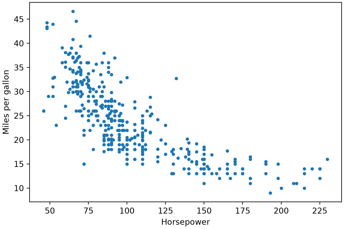
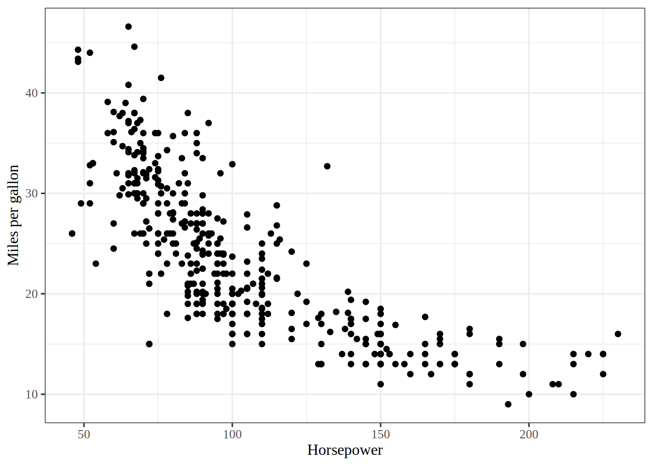
The correlation is -0.78, so cars with more horsepower tend to get fewer miles per gallon. Horsepower is a strong candidate predictor of mpg for the models in this lab.
ExrExercise 3 (Lab: a histogram of fuel efficiency)
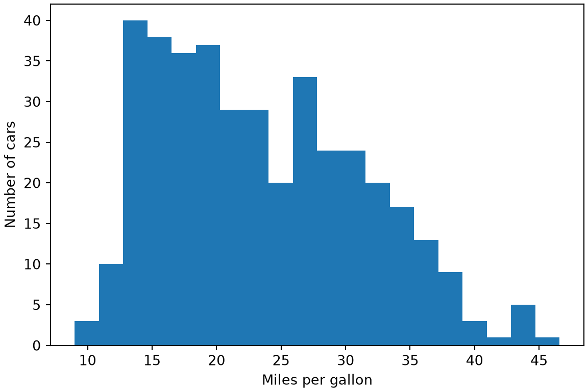
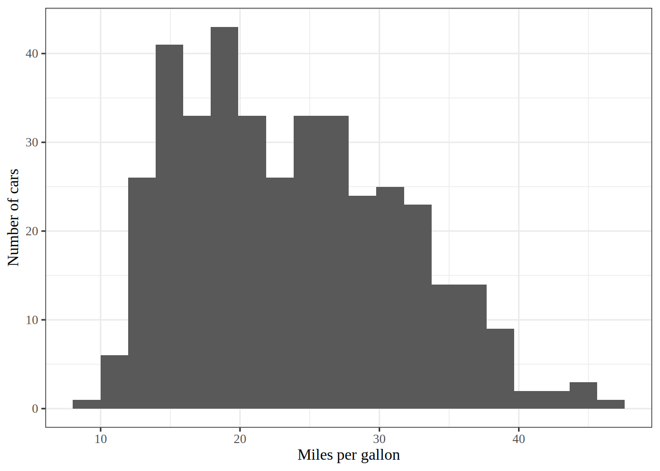
Exercise 3 (Lab: a histogram of fuel efficiency) Use the Auto data. Draw a histogram of mpg.
import matplotlib.pyplot as pltfig, ax = plt.subplots(figsize=(6, 4), layout="constrained")ax.hist(auto_eda_py["mpg"], bins=20);ax.set_xlabel("Miles per gallon");ax.set_ylabel("Number of cars");plt.show()
library(ggplot2)# nolint: undesirable_function_lintermpg_histogram<-auto_eda_r|>ggplot()+aes(mpg)+geom_histogram(bins =20)+labs(x ="Miles per gallon", y ="Number of cars")mpg_histogram
I chose 20 bins, which is about 20 cars per bar on average. Far fewer bins would hide the shape inside a few wide bars, and far more would leave most bars with only a few cars, so the outline would look ragged. That is why 20 is a compromise between the two.
import matplotlib.pyplot as pltfig, ax = plt.subplots(figsize=(6, 4), layout="constrained")ax.scatter(auto_eda_py["horsepower"], auto_eda_py["mpg"], s=10);ax.set_xlabel("Horsepower");ax.set_ylabel("Miles per gallon");plt.show()
library(ggplot2)# nolint: undesirable_function_lintermpg_horsepower_plot<-auto_eda_r|>ggplot()+aes(horsepower, mpg)+geom_point()+labs(x ="Horsepower", y ="Miles per gallon")mpg_horsepower_plot
Figure 2 shows miles per gallon falling as horsepower rises.
The points follow a curve, not a straight line, so a straight-line model leaves a systematic pattern, which is the reason the lab goes on to add a squared horsepower term.
3 The validation set approach
ExrExercise 5 (Lab: split the data into two halves)
# Fix the seed so the random split is the same on every render;# seed 1 is the book's, so this tab draws the book's split.set.seed(1)auto<-readr::read_csv("data/auto.csv", show_col_types =FALSE)# Draw 196 of the 392 row numbers, without repeats, for the training set;# the other 196 rows are the validation set.train<-sample(392, 196)length(train)
# Fit the line on the training rows only.lm_fit<-lm(mpg~horsepower, data =auto, subset =train)# Predict every car, then keep the squared errors of the validation rows.lm_pred<-predict(lm_fit, auto)lm_sq_err<-(auto$mpg-lm_pred)^2lin_base_mse<-mean(lm_sq_err[-train])lin_base_mse
[1] 23.26601
lin_spec<-linear_reg()lin_fit<-fit(lin_spec, mpg~horsepower, data =auto_train)lin_pred<-predict(lin_fit, auto_valid)lin_r_mse<-mean((auto_valid$mpg-lin_pred$.pred)^2)lin_r_mse
[1] 23.26601
The validation error is 23.27 in each R run and 23.6 in the Python run. From seed 1, sample() and initial_split() put the same \(196\) cars in the training set, which is the book’s split, so both R runs match the book’s value of 23.27 [3, Sec. 5.3.1]. Python’s generator draws a different split, so its number differs.
ExrExercise 7 (Lab: find the validation error of a quadratic fit)
# I() makes ^ square horsepower, instead of meaning a formula interaction.lm_fit2<-lm(mpg~horsepower+I(horsepower^2), data =auto, subset =train)# Score the quadratic fit on the same validation rows as the line.lm_pred2<-predict(lm_fit2, auto)lm_sq_err2<-(auto$mpg-lm_pred2)^2quad_base_mse<-mean(lm_sq_err2[-train])quad_base_mse
[1] 18.71646
quad_fit<-fit(lin_spec, mpg~horsepower+I(horsepower^2), data =auto_train)quad_pred<-predict(quad_fit, auto_valid)quad_r_mse<-mean((auto_valid$mpg-quad_pred$.pred)^2)quad_r_mse
[1] 18.71646
The fit with the squared term has validation error 18.7 in each R run and 18.8 in the Python run, below the straight line’s 23.3 and 23.6. The relationship between horsepower and mpg curves, which a line cannot follow.
4 Cross-validation
ExrExercise 8 (Lab: find the ten-fold cross-validation error)
# Fix the seed so the folds are the same on every render; 17 is the book's seed.set.seed(17)# glm() without a family fits the same line as lm(),# in the form that boot::cv.glm() accepts.glm_fit<-glm(mpg~horsepower, data =auto)cv_err_ten<-boot::cv.glm(auto, glm_fit, K =10)# The first element of delta is the cross-validation estimate of the MSE.cv_base_mse<-cv_err_ten$delta[1]cv_base_mse
[1] 24.27207
auto_folds<-vfold_cv(auto, v =10)rmse_only<-metric_set(rmse)cv_res<-fit_resamples(lin_spec,mpg~horsepower, resamples =auto_folds, metrics =rmse_only)cv_metrics<-collect_metrics(cv_res, summarize =FALSE)cv_r_mse<-mean(cv_metrics$.estimate^2)cv_r_mse
[1] 24.41096
The cross-validation estimate is 24.3 in the R run, 24.4 in the tidymodels run, and 24.2 in the Python run. It uses every observation for both fitting and validation, so it depends less on any one random split than a single validation error does.
ExrExercise 9 (Lab: find the leave-one-out cross-validation error)
# glm() without a family fits the same line as lm(),# in the form that boot::cv.glm() accepts.glm_fit<-glm(mpg~horsepower, data =auto)# With no K, cv.glm() leaves out one observation at a time.cv_err<-boot::cv.glm(auto, glm_fit)# The first element of delta is the cross-validation estimate of the MSE.loo_base_mse<-cv_err$delta[1]loo_base_mse
[1] 24.23151
auto_loo<-loo_cv(auto)loo_spec<-linear_reg()loo_squared_error<-purrr::map_dbl(auto_loo$splits, \(split){left_in<-analysis(split)loo_fit<-fit(loo_spec, mpg~horsepower, data =left_in)left_out<-assessment(split)loo_pred<-predict(loo_fit, left_out)(left_out$mpg-loo_pred$.pred)^2})loo_r_mse<-mean(loo_squared_error)loo_r_mse
[1] 24.23151
The leave-one-out cross-validationestimate is 24.2 in each R run and 24.2 in the Python run. The tidymodels code makes each fit itself, because tune does not accept leave-one-out resamples. Each of the \(392\) fits leaves out one observation. No random split is involved, so the three runs agree.
5 The bootstrap
ExrExercise 10 (Lab: estimate a standard error with the bootstrap)
# Fix the seed so the bootstrap samples are the same on every render.set.seed(1)# boot::boot() calls the function once per bootstrap sample,# passing the row numbers that the sample drew;# the function returns the intercept and the slope fitted to those rows,# as the book's boot.fn() does.boot_out<-boot::boot(auto, \(data, index){boot_lm<-lm(mpg~horsepower, data =data, subset =index)coef(boot_lm)}, 1000)# Column 2 of t holds the 1000 bootstrap slopes.boot_se_base<-sd(boot_out$t[, 2])boot_out
set.seed(0)auto_boot<-bootstraps(auto, times =1000)boot_spec<-linear_reg()boot_slopes<-purrr::map_dbl(auto_boot$splits, \(split){boot_data<-analysis(split)boot_fit<-fit(boot_spec, mpg~horsepower, data =boot_data)tidy(boot_fit)$estimate[2]})boot_se_r<-sd(boot_slopes)boot_se_r
[1] 0.007477015
The bootstrap standard error of the slope is about 0.0074 in the R run, 0.0075 in the tidymodels run, and 0.0075 in the Python run. Each run draws its own random bootstrap samples, so the three values agree only approximately.
References
[1]
G. James, D. Witten, T. Hastie, R. Tibshirani, and J. Taylor, An introduction to statistical learning: With applications in Python. Springer, 2023. doi: 10.1007/978-3-031-38747-0.
[2]
F. Pedregosa et al., “Scikit-learn: Machine learning in Python,”Journal of Machine Learning Research, vol. 12, pp. 2825–2830, 2011, Available: https://jmlr.org/papers/v12/pedregosa11a.html
[3]
G. James, D. Witten, T. Hastie, and R. Tibshirani, An introduction to statistical learning with applications in R, 2nd ed. Springer, 2021. Available: https://www.statlearning.com/