Resampling Lab

Last modified: 2026-11-19

Show code
# The Python chunks on this page import matplotlib, numpy, pandas
# and scikit-learn; reticulate provisions them.
py_packages <- c("matplotlib", "numpy", "pandas", "scikit-learn")
library(reticulate) # nolint: undesirable_function_linter
library(tidymodels) # nolint: undesirable_function_linter
py_require(py_packages)

1 The book’s Chapter 5 lab

This page holds the code lab for the Model Selection chapter.

To work the lab without the solutions, download a stub with only the exercises:

Each solution shows the code in Python, in R as the book’s lab writes it, and in R with tidymodels.

Section 5.3 of the book [1] is the source of these exercises. The Python code follows the book’s Chapter 5 lab notebook, with scikit-learn [2] in place of the ISLP package. The R code without tidymodels follows the book’s Chapter 5 R lab [3, Sec. 5.3], with lm(), boot::cv.glm() and boot::boot(). The tidymodels code fits the same models with tidymodels.

2 Exploring the Auto data

Exercise 1 (Lab: the average fuel efficiency)

Exercise 1 (Lab: the average fuel efficiency) Use the Auto data [1]. What is the sample mean of mpg?

Hint

A summary of a column of the data frame returns its sample mean.

Solution 1.

import pandas as pd

auto_eda_py = pd.read_csv("data/auto.csv")
auto_eda_py_mean = float(auto_eda_py["mpg"].mean())
round(auto_eda_py_mean, 2)
23.45
auto_eda_r <- readr::read_csv("data/auto.csv", show_col_types = FALSE)
auto_eda_r_mean <- mean(auto_eda_r$mpg)
round(auto_eda_r_mean, 2)
[1] 23.45

The cars in the Auto data average 23.4 miles per gallon.

Exercise 2 (Lab: fuel efficiency and horsepower)

Exercise 2 (Lab: fuel efficiency and horsepower) Use the Auto data. What is the sample correlation between mpg and horsepower?

Hint

The summary functions of a data frame include its correlation matrix, from which you read one pair of columns.

Solution 2. This solution continues Solution 1.

auto_eda_py_cor = float(auto_eda_py["mpg"].corr(auto_eda_py["horsepower"]))
round(auto_eda_py_cor, 3)
-0.778
auto_eda_r_cor <- cor(auto_eda_r$mpg, auto_eda_r$horsepower)
round(auto_eda_r_cor, 3)
[1] -0.778

The correlation is -0.78, so cars with more horsepower tend to get fewer miles per gallon. Horsepower is a strong candidate predictor of mpg for the models in this lab.

Exercise 3 (Lab: a histogram of fuel efficiency)

Exercise 3 (Lab: a histogram of fuel efficiency) Use the Auto data. Draw a histogram of mpg.

Hint

The plotting functions draw a histogram of one column.

Solution 3. This solution continues Solution 1.

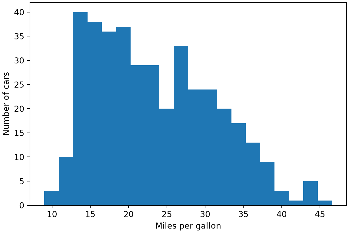
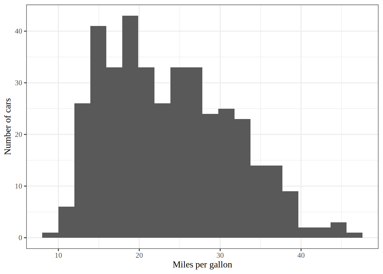
Figure 1: Bars counting the cars at each level of miles per gallon.
import matplotlib.pyplot as plt

fig, ax = plt.subplots(figsize=(6, 4), layout="constrained")
ax.hist(auto_eda_py["mpg"], bins=20);
ax.set_xlabel("Miles per gallon");
ax.set_ylabel("Number of cars");
plt.show()

Histogram of miles per gallon for the cars in the data. The tallest bars are at the low-to-middle values, and the bars shrink toward a thin tail at the highest values.

library(ggplot2) # nolint: undesirable_function_linter

mpg_histogram <- auto_eda_r |>
  ggplot() +
  aes(mpg) +
  geom_histogram(bins = 20) +
  labs(x = "Miles per gallon", y = "Number of cars")
mpg_histogram

Histogram of miles per gallon for the cars in the data. The tallest bars are at the low-to-middle values, and the bars shrink toward a thin tail at the highest values.

Show code
auto_eda_r_median <- median(auto_eda_r$mpg)
auto_eda_r_per_bin <- nrow(auto_eda_r) / 20

I chose 20 bins, which is about 20 cars per bar on average. Far fewer bins would hide the shape inside a few wide bars, and far more would leave most bars with only a few cars, so the outline would look ragged. That is why 20 is a compromise between the two.

Figure 1 shows a mildly right-skewed shape: the sample median is 22.75, below the sample mean of 23.4.

Exercise 4 (Lab: a scatterplot of fuel efficiency against horsepower)

Exercise 4 (Lab: a scatterplot of fuel efficiency against horsepower) Use the Auto data. Draw a scatterplot of mpg against horsepower.

Hint

The plotting functions draw a scatterplot of one column against another.

Solution 4. This solution continues Solution 1.

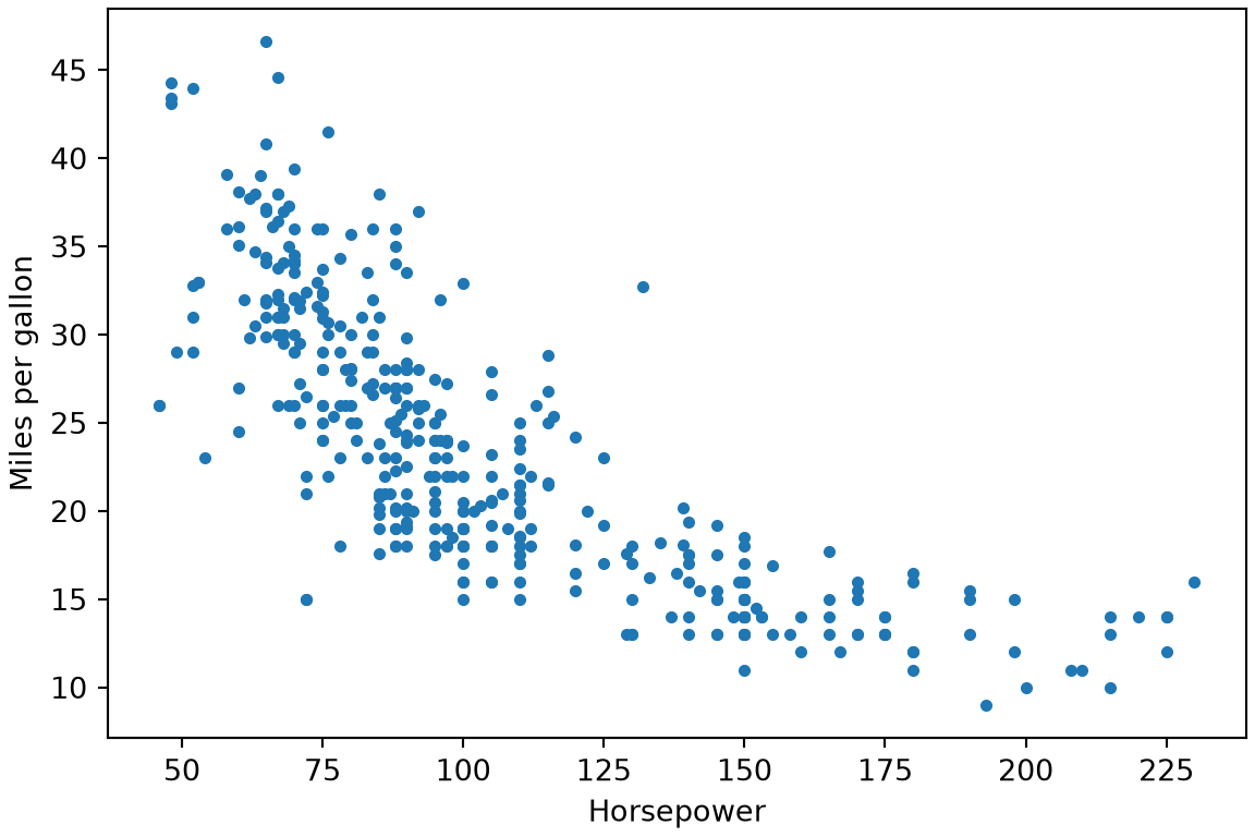
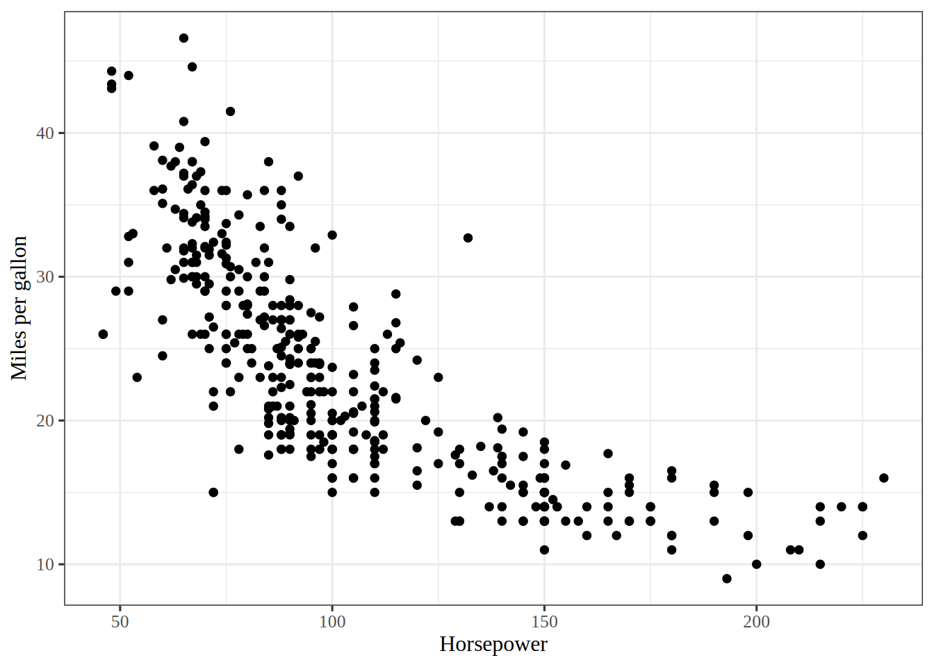
Figure 2: Miles per gallon against horsepower, with one dot per car.
import matplotlib.pyplot as plt

fig, ax = plt.subplots(figsize=(6, 4), layout="constrained")
ax.scatter(auto_eda_py["horsepower"], auto_eda_py["mpg"], s=10);
ax.set_xlabel("Horsepower");
ax.set_ylabel("Miles per gallon");
plt.show()

Scatterplot of miles per gallon against horsepower. The points fall from the upper left to the lower right, along a curve that is steep at low horsepower and flattens at high horsepower.

library(ggplot2) # nolint: undesirable_function_linter

mpg_horsepower_plot <- auto_eda_r |>
  ggplot() +
  aes(horsepower, mpg) +
  geom_point() +
  labs(x = "Horsepower", y = "Miles per gallon")
mpg_horsepower_plot

Scatterplot of miles per gallon against horsepower. The points fall from the upper left to the lower right, along a curve that is steep at low horsepower and flattens at high horsepower.

Figure 2 shows miles per gallon falling as horsepower rises.

The points follow a curve, not a straight line, so a straight-line model leaves a systematic pattern, which is the reason the lab goes on to add a squared horsepower term.

3 The validation set approach

Exercise 5 (Lab: split the data into two halves)

Exercise 5 (Lab: split the data into two halves) Randomly split the \(392\) observations of the Auto data [1] into a training set of \(196\) observations and a validation set of \(196\).

Hint

The random number functions draw whole numbers with or without repeats, and a selection by position keeps those rows of the data frame.

Solution 5.

import pandas as pd
from sklearn.model_selection import train_test_split

auto = pd.read_csv("data/auto.csv")
auto_train, auto_valid = train_test_split(auto, train_size=196, random_state=0)
auto_train.shape, auto_valid.shape
((196, 9), (196, 9))
Show code
# Fix the seed so the random split is the same on every render;
# seed 1 is the book's, so this tab draws the book's split.
set.seed(1)
auto <- readr::read_csv("data/auto.csv", show_col_types = FALSE)
# Draw 196 of the 392 row numbers, without repeats, for the training set;
# the other 196 rows are the validation set.
train <- sample(392, 196)
length(train)
[1] 196
set.seed(1)
auto <- readr::read_csv("data/auto.csv", show_col_types = FALSE)
auto_split <- initial_split(auto, prop = 0.5)
auto_train <- training(auto_split)
auto_valid <- testing(auto_split)
n_train <- nrow(auto_train)
n_valid <- nrow(auto_valid)
c(n_train, n_valid)
[1] 196 196

Exercise 6 (Lab: find the validation error of a linear fit)

Exercise 6 (Lab: find the validation error of a linear fit) Fit a linear regression of mpg on horsepower to the training set of Solution 5, and find the mean squared error of its predictions on the validation set.

Hint

Fit a model with a formula on the training set, predict on the validation set, and take the mean of the squared differences, as the error function of scikit-learn does.

Solution 6.

from sklearn.linear_model import LinearRegression

lin_py = LinearRegression()
lin_py = lin_py.fit(auto_train[["horsepower"]], auto_train["mpg"])
lin_py_pred = lin_py.predict(auto_valid[["horsepower"]])
lin_py_mse = float(((auto_valid["mpg"] - lin_py_pred) ** 2).mean())
lin_py_mse
23.61661706966988
Show code
# Fit the line on the training rows only.
lm_fit <- lm(mpg ~ horsepower, data = auto, subset = train)
# Predict every car, then keep the squared errors of the validation rows.
lm_pred <- predict(lm_fit, auto)
lm_sq_err <- (auto$mpg - lm_pred)^2
lin_base_mse <- mean(lm_sq_err[-train])
lin_base_mse
[1] 23.26601
lin_spec <- linear_reg()
lin_fit <- fit(lin_spec, mpg ~ horsepower, data = auto_train)
lin_pred <- predict(lin_fit, auto_valid)
lin_r_mse <- mean((auto_valid$mpg - lin_pred$.pred)^2)
lin_r_mse
[1] 23.26601

The validation error is 23.27 in each R run and 23.6 in the Python run. From seed 1, sample() and initial_split() put the same \(196\) cars in the training set, which is the book’s split, so both R runs match the book’s value of 23.27 [3, Sec. 5.3.1]. Python’s generator draws a different split, so its number differs.

Exercise 7 (Lab: find the validation error of a quadratic fit)

Exercise 7 (Lab: find the validation error of a quadratic fit) Fit a quadratic linear regression of mpg on horsepower to the training set of Solution 5, and find the mean squared error of its predictions on the validation set.

Hint

Wrap the square in I(...) inside the formula, then compute the mean squared error on the validation set as in Exercise 6.

Solution 7.

from sklearn.pipeline import make_pipeline
from sklearn.preprocessing import PolynomialFeatures

quad_py = make_pipeline(PolynomialFeatures(2), LinearRegression())
quad_py = quad_py.fit(auto_train[["horsepower"]], auto_train["mpg"])
quad_py_pred = quad_py.predict(auto_valid[["horsepower"]])
quad_py_mse = float(((auto_valid["mpg"] - quad_py_pred) ** 2).mean())
quad_py_mse
18.763031346897684
Show code
# I() makes ^ square horsepower, instead of meaning a formula interaction.
lm_fit2 <- lm(mpg ~ horsepower + I(horsepower^2), data = auto, subset = train)
# Score the quadratic fit on the same validation rows as the line.
lm_pred2 <- predict(lm_fit2, auto)
lm_sq_err2 <- (auto$mpg - lm_pred2)^2
quad_base_mse <- mean(lm_sq_err2[-train])
quad_base_mse
[1] 18.71646
quad_fit <- fit(lin_spec, mpg ~ horsepower + I(horsepower^2), data = auto_train)
quad_pred <- predict(quad_fit, auto_valid)
quad_r_mse <- mean((auto_valid$mpg - quad_pred$.pred)^2)
quad_r_mse
[1] 18.71646

The fit with the squared term has validation error 18.7 in each R run and 18.8 in the Python run, below the straight line’s 23.3 and 23.6. The relationship between horsepower and mpg curves, which a line cannot follow.

4 Cross-validation

Exercise 8 (Lab: find the ten-fold cross-validation error)

Exercise 8 (Lab: find the ten-fold cross-validation error) Find the ten-fold cross-validation estimate of the mean squared error of linear regression of mpg on horsepower, using all \(392\) observations of the Auto data.

Hint

Split the row numbers into ten groups; each group is held out once while the model is fit on the rest.

Solution 8.

from sklearn.model_selection import KFold, cross_val_score

folds_py = KFold(10, shuffle=True, random_state=0)
cv_py_scores = cross_val_score(
    LinearRegression(),
    auto[["horsepower"]],
    auto["mpg"],
    cv=folds_py,
    scoring="neg_mean_squared_error",
)
cv_py_mse = float(-cv_py_scores.mean())
cv_py_mse
24.207664490171332
Show code
# Fix the seed so the folds are the same on every render; 17 is the book's seed.
set.seed(17)
# glm() without a family fits the same line as lm(),
# in the form that boot::cv.glm() accepts.
glm_fit <- glm(mpg ~ horsepower, data = auto)
cv_err_ten <- boot::cv.glm(auto, glm_fit, K = 10)
# The first element of delta is the cross-validation estimate of the MSE.
cv_base_mse <- cv_err_ten$delta[1]
cv_base_mse
[1] 24.27207
auto_folds <- vfold_cv(auto, v = 10)
rmse_only <- metric_set(rmse)
cv_res <- fit_resamples(
  lin_spec,
  mpg ~ horsepower,
  resamples = auto_folds,
  metrics = rmse_only
)
cv_metrics <- collect_metrics(cv_res, summarize = FALSE)
cv_r_mse <- mean(cv_metrics$.estimate^2)
cv_r_mse
[1] 24.41096

The cross-validation estimate is 24.3 in the R run, 24.4 in the tidymodels run, and 24.2 in the Python run. It uses every observation for both fitting and validation, so it depends less on any one random split than a single validation error does.

Exercise 9 (Lab: find the leave-one-out cross-validation error)

Exercise 9 (Lab: find the leave-one-out cross-validation error) Using leave-one-out cross-validation, find the cross-validation estimate of the mean squared error of linear regression of mpg on horsepower, using all \(392\) observations of the Auto data.

Hint

Hold out one row at a time, fit the model on the rest, and average the squared errors of the predictions.

Solution 9.

from sklearn.linear_model import LinearRegression
from sklearn.model_selection import LeaveOneOut, cross_val_score

loo_py_scores = cross_val_score(
    LinearRegression(),
    auto[["horsepower"]],
    auto["mpg"],
    cv=LeaveOneOut(),
    scoring="neg_mean_squared_error",
)
loo_py_mse = float(-loo_py_scores.mean())
loo_py_mse
24.231513517929226
Show code
# glm() without a family fits the same line as lm(),
# in the form that boot::cv.glm() accepts.
glm_fit <- glm(mpg ~ horsepower, data = auto)
# With no K, cv.glm() leaves out one observation at a time.
cv_err <- boot::cv.glm(auto, glm_fit)
# The first element of delta is the cross-validation estimate of the MSE.
loo_base_mse <- cv_err$delta[1]
loo_base_mse
[1] 24.23151
auto_loo <- loo_cv(auto)
loo_spec <- linear_reg()
loo_squared_error <- purrr::map_dbl(auto_loo$splits, \(split) {
  left_in <- analysis(split)
  loo_fit <- fit(loo_spec, mpg ~ horsepower, data = left_in)
  left_out <- assessment(split)
  loo_pred <- predict(loo_fit, left_out)
  (left_out$mpg - loo_pred$.pred)^2
})
loo_r_mse <- mean(loo_squared_error)
loo_r_mse
[1] 24.23151

The leave-one-out cross-validation estimate is 24.2 in each R run and 24.2 in the Python run. The tidymodels code makes each fit itself, because tune does not accept leave-one-out resamples. Each of the \(392\) fits leaves out one observation. No random split is involved, so the three runs agree.

5 The bootstrap

Exercise 10 (Lab: estimate a standard error with the bootstrap)

Exercise 10 (Lab: estimate a standard error with the bootstrap) Draw \(1000\) bootstrap samples of the \(392\) observations of the Auto data. In each, fit a linear regression of mpg on horsepower. Use the slope from each of the \(1000\) fits to find the bootstrap standard error of the slope.

Hint

Draw each of the bootstrap samples with rng.choice or rng.integers in Python, or boot::boot() or rsample::bootstraps() in R, then take the standard deviation of the slopes.

Solution 10.

import numpy as np
from sklearn.linear_model import LinearRegression

rng = np.random.default_rng(0)
n_obs_py = len(auto)
slopes_py = np.empty(1000)
for b in range(1000):
    rows_py = rng.integers(0, n_obs_py, size=n_obs_py)
    boot_py = auto.iloc[rows_py]
    boot_fit_py = LinearRegression().fit(boot_py[["horsepower"]], boot_py["mpg"])
    slopes_py[b] = boot_fit_py.coef_[0]
boot_se_py = float(slopes_py.std(ddof=1))
boot_se_py
0.00746209301139544
Show code
# Fix the seed so the bootstrap samples are the same on every render.
set.seed(1)
# boot::boot() calls the function once per bootstrap sample,
# passing the row numbers that the sample drew;
# the function returns the intercept and the slope fitted to those rows,
# as the book's boot.fn() does.
boot_out <- boot::boot(auto, \(data, index) {
  boot_lm <- lm(mpg ~ horsepower, data = data, subset = index)
  coef(boot_lm)
}, 1000)
# Column 2 of t holds the 1000 bootstrap slopes.
boot_se_base <- sd(boot_out$t[, 2])
boot_out

ORDINARY NONPARAMETRIC BOOTSTRAP


Call:
boot::boot(data = auto, statistic = function(data, index) {
    boot_lm <- lm(mpg ~ horsepower, data = data, subset = index)
    coef(boot_lm)
}, R = 1000)


Bootstrap Statistics :
      original        bias    std. error
t1* 39.9358610  0.0553942585 0.843931305
t2* -0.1578447 -0.0006285291 0.007367396
set.seed(0)
auto_boot <- bootstraps(auto, times = 1000)
boot_spec <- linear_reg()
boot_slopes <- purrr::map_dbl(auto_boot$splits, \(split) {
  boot_data <- analysis(split)
  boot_fit <- fit(boot_spec, mpg ~ horsepower, data = boot_data)
  tidy(boot_fit)$estimate[2]
})
boot_se_r <- sd(boot_slopes)
boot_se_r
[1] 0.007477015

The bootstrap standard error of the slope is about 0.0074 in the R run, 0.0075 in the tidymodels run, and 0.0075 in the Python run. Each run draws its own random bootstrap samples, so the three values agree only approximately.

References

[1]
G. James, D. Witten, T. Hastie, R. Tibshirani, and J. Taylor, An introduction to statistical learning: With applications in Python. Springer, 2023. doi: 10.1007/978-3-031-38747-0.
[2]
F. Pedregosa et al., “Scikit-learn: Machine learning in Python,” Journal of Machine Learning Research, vol. 12, pp. 2825–2830, 2011, Available: https://jmlr.org/papers/v12/pedregosa11a.html
[3]
G. James, D. Witten, T. Hastie, and R. Tibshirani, An introduction to statistical learning with applications in R, 2nd ed. Springer, 2021. Available: https://www.statlearning.com/