Subset Selection

Published

Last modified: 2026-11-19

Show code
# The Python chunks import numpy, pandas, matplotlib, scipy, statsmodels
# and l0bnb; reticulate provisions them.
py_packages <- c("numpy", "pandas", "matplotlib", "scipy", "statsmodels",
                 "l0bnb")
library(reticulate) # nolint: undesirable_function_linter
py_require(py_packages)

1 How many models?

ExrExercise 1 (How many models?)

Exercise 1 (How many models?) Each model below keeps the intercept and uses some subset of \(p\) candidate features.

How many such models are there?

Solution 1. Each feature is either in the model or out of it, so there are \(2^p\) models.

ExrExercise 2 (How many models? (part 2))

Exercise 2 (How many models? (part 2)) Use the setup of Exercise 1.

How many are there for \(8\) features, and for \(30\)?

Solution 2. For \(p = 8\) there are \(2^8 = 256\) models, few enough to fit them all. For \(p = 30\) there are \(2^{30} =\) 1,073,741,824 models, too many to fit [1, Sec. 3.2.2], p. 87. The procedures that follow fit far fewer.

2 Forward and backward selection

Examples on the Auto data in this chapter use the objects below. The section Lab: linear regression on the Auto data builds the same objects step by step.

Show code
import numpy as np
import pandas as pd
from scipy import stats

# ISLP's load_data("Auto") reads this same file.
Auto = pd.read_csv("data/auto.csv")
y = Auto["mpg"].to_numpy()
n = len(y)

# Indicators of a European and of a Japanese car; American is the baseline.
origin = Auto["origin"].to_numpy()
european = (origin == 2).astype(float)
japanese = (origin == 3).astype(float)


def fit(columns):
    """Least-squares coefficients of mpg on an intercept and `columns`."""
    Phi = np.column_stack([np.ones(n)] + columns)
    beta_hat = np.linalg.lstsq(Phi, y, rcond=None)[0]
    return beta_hat, Phi
Show code
auto <- readr::read_csv("data/auto.csv", show_col_types = FALSE)
DefDefinition 1 (Forward selection)

Definition 1 (Forward selection) Forward selection starts from the model with only an intercept. At each step, it fits every model that adds one more feature, and keeps the one with the lowest residual sum of squares (RSS). It stops when a stopping rule is met [1, Sec. 3.2.2], p. 87, [3].

ExmExample 1 (Forward selection on the Auto data)

Example 1 (Forward selection on the Auto data) Run forward selection (Definition 1) for mpg over eight candidate features: cylinders, displacement, horsepower, weight, acceleration, year, and the european and japanese indicators of the exercise Lab: use a category as a feature. Record the order in which the features enter and the RSS after each step.

candidates = {
    name: Auto[name].to_numpy(float)
    for name in ["cylinders", "displacement", "horsepower", "weight",
                 "acceleration", "year"]
}
candidates["european"] = european
candidates["japanese"] = japanese

def rss(names):
    beta_hat, Phi = fit([candidates[k] for k in names])
    return np.sum((y - Phi @ beta_hat) ** 2)

forward_order, forward_rss = [], []
remaining = list(candidates)
while remaining:
    best = min(remaining, key=lambda k: rss(forward_order + [k]))
    forward_order.append(best)
    remaining.remove(best)
    forward_rss.append(rss(forward_order))
print(pd.DataFrame({"added": forward_order, "rss": forward_rss}))
          added          rss
0        weight  7321.233706
1          year  4568.952042
2      japanese  4472.554527
3      european  4310.409498
4  displacement  4271.964759
5    horsepower  4221.333733
6     cylinders  4194.483283
7  acceleration  4187.391678
auto <- dplyr::mutate(auto,
                       european = as.numeric(origin == 2),
                       japanese = as.numeric(origin == 3))
candidates <- c("cylinders", "displacement", "horsepower", "weight",
                "acceleration", "year", "european", "japanese")

rss <- function(names, data) {
  fit <- lm(reformulate(names, response = "mpg"), data = data)
  sum(residuals(fit)^2)
}

forward_order <- character(0)
forward_rss <- numeric(0)
remaining <- candidates
while (length(remaining) > 0) {
  scores <- sapply(remaining, function(k) rss(c(forward_order, k), auto))
  best <- names(which.min(scores))
  forward_order <- c(forward_order, best)
  forward_rss <- c(forward_rss, min(scores))
  remaining <- setdiff(remaining, best)
}
tibble::tibble(added = forward_order, rss = forward_rss)

R also has built-in tools for this search. add1() fits each one-feature addition to a model and reports its RSS:

null_fit <- lm(mpg ~ 1, data = auto)
full_formula <- reformulate(candidates, response = "mpg")
add1(null_fit, scope = full_formula)

step() calls add1() repeatedly, but it orders the candidates by the AIC, not by RSS, \(p\)-values or cross-validation, and it stops as soon as no addition lowers the AIC. Its option k is the penalty per coefficient: the default k = 2 gives the AIC, and k = log(n) gives the BIC. Among the candidates that add one feature to the same model, the one with the lowest AIC has the lowest RSS, so step() adds features in the same order as the loop above. Setting k = 0 removes the penalty, so the search runs until every feature is in:

forward_all <- step(null_fit, scope = full_formula,
                    direction = "forward", k = 0, trace = 0)
forward_all$anova
forward_all_steps <- forward_all$anova$Step[-1]
forward_all_order <- sub("+ ", "", forward_all_steps, fixed = TRUE)
all(forward_all_order == forward_order)
[1] TRUE

With the default k = 2, the search stops early:

forward_aic <- step(null_fit, scope = full_formula,
                    direction = "forward", trace = 0)
forward_aic$anova
forward_aic_terms <- terms(forward_aic)
forward_aic_kept <- attr(forward_aic_terms, "term.labels")
forward_aic_left_out <- setdiff(candidates, forward_aic_kept)
forward_aic_left_out
[1] "acceleration"

The AIC search keeps 7 features and leaves out acceleration, the last feature that the loop added. MASS::stepAIC() runs the same search.

weight enters first, with RSS 7321, then year, which brings it down to 4569. After that the gains are small: the last 6 features together lower the RSS only to 4187. The RSS falls at every step, as the solution to the exercise Lab: add a second feature shows it must, so it cannot by itself say when to stop. These are training RSS values, computed on the cars used to fit, so they get no confidence intervals: the residuals are not independent draws, and the values are biased low.

DefDefinition 2 (Backward selection)

Definition 2 (Backward selection) Backward selection starts from the model with all \(p\) features. At each step, it removes the feature whose \(t\)-test gives the largest \(p\)-value and refits. It stops when a stopping rule is met, such as every remaining \(p\)-value being below a threshold [1, Sec. 3.2.2], p. 87, [3].

ExmExample 2 (Backward selection on the Auto data)

Example 2 (Backward selection on the Auto data) Run backward selection (Definition 2) over the eight features of Example 1, stopping when every remaining \(p\)-value is below \(0.05\).

def p_values(names):
    beta_hat, Phi = fit([candidates[k] for k in names])
    df = n - Phi.shape[1]
    sigma2 = np.sum((y - Phi @ beta_hat) ** 2) / df
    se = np.sqrt(sigma2 * np.diag(np.linalg.inv(Phi.T @ Phi)))
    return 2 * stats.t.sf(np.abs(beta_hat / se), df)[1:]

backward_kept = list(candidates)
backward_dropped, backward_p = [], []
while np.max(p_values(backward_kept)) >= 0.05:
    p = p_values(backward_kept)
    backward_dropped.append(backward_kept[np.argmax(p)])
    backward_p.append(np.max(p))
    backward_kept.remove(backward_dropped[-1])
print(pd.DataFrame({"dropped": backward_dropped, "p": backward_p}))
        dropped         p
0  acceleration  0.421101
1     cylinders  0.117742
print(backward_kept)
['displacement', 'horsepower', 'weight', 'year', 'european', 'japanese']
backward_kept <- candidates
repeat {
  fit <- lm(reformulate(backward_kept, response = "mpg"), data = auto)
  p <- coef(summary(fit))[-1, 4]
  if (max(p) < 0.05) break
  print(c(dropped = names(which.max(p)), p = signif(max(p), 2)))
  backward_kept <- setdiff(backward_kept, names(which.max(p)))
}
       dropped              p 
"acceleration"         "0.42" 
    dropped           p 
"cylinders"      "0.12" 
backward_kept
[1] "displacement" "horsepower"   "weight"       "year"         "european"    
[6] "japanese"    

drop1() is R’s built-in tool for one backward step. With test = "F", it tests the removal of each feature with an \(F\)-test. For a feature with one coefficient, the \(F\)-test and the \(t\)-test give the same \(p\)-value, so drop1() reports the \(p\)-values that the loop above uses:

full_fit <- lm(full_formula, data = auto)
drop1(full_fit, test = "F")

step() with direction = "backward" repeats that step, but it orders the removals by the AIC, not by \(p\)-values, and stops when no removal lowers the AIC:

backward_aic <- step(full_fit, direction = "backward", trace = 0)
backward_aic$anova
backward_aic_terms <- terms(backward_aic)
backward_aic_kept <- attr(backward_aic_terms, "term.labels")
backward_aic_kept
[1] "cylinders"    "displacement" "horsepower"   "weight"       "year"        
[6] "european"     "japanese"    

The AIC search keeps 7 features, 1 more than the \(p\)-value loop. An AIC penalty of \(2\) per coefficient is a looser bar than a \(p\)-value below \(0.05\): with many cars, removing one coefficient raises the AIC when its \(\abs{t} > \sqrt{2}\), which is roughly \(p < 0.16\). So a feature can lower the AIC without being significant at the \(0.05\) level.

Backward selection drops acceleration (\(p = 0.42\)) and then cylinders (\(p = 0.12\)), and keeps 6 features: displacement, horsepower, weight, year, european, japanese. Forward selection added those same two features last, so here the two procedures agree on which features matter least. They need not agree in general.

RemarkRemark 1 (Mixed selection, and choosing when to stop)

Remark 1 (Mixed selection, and choosing when to stop). Mixed selection adds features as forward selection does, but after each step it removes any feature whose \(p\)-value has risen above a threshold. It can drop a feature that forward selection added early and that later became redundant. In R, step() and MASS::stepAIC() with direction = "both" run a version of mixed selection that at each step adds or drops whichever feature lowers the AIC the most. Backward selection needs \(p < n\), since it starts by fitting every feature; forward selection does not [1, Sec. 3.2.2], p. 87.

None of the three procedures is guaranteed to find the best of the \(2^p\) models. A stopping rule based on training error alone always takes the largest model, as Example 1 shows. Model Selection chooses with cross-validation instead.

3 Best subset selection

ExrExercise 3 (Finding the best model of each size for certain)

Exercise 3 (Finding the best model of each size for certain) Forward selection and backward selection each fit only some of the \(2^{\ninputvars}\) models that use a subset of \(\ninputvars\) candidate features, so neither is guaranteed to find, for a given number of features \(\subsetsize\), the model with the smallest residual sum of squares among all models with \(\subsetsize\) features.

TipHint

Use the count of models in Solution 1.

Describe a way to find that model for every \(\subsetsize\) from \(0\) to \(\ninputvars\) with certainty.

Solution 3. Fit every model that uses a subset of the \(\ninputvars\) candidate features. Then, for each number of features \(\subsetsize\), keep the fitted model with the smallest residual sum of squares among those with \(\subsetsize\) features. No model is skipped, so the kept model is the best one of its size. The residual sum of squares compares only models of the same size: it never rises when a feature is added, so a different criterion has to choose among the \(\ninputvars + 1\) kept models.

DefDefinition 3 (Best subset selection)

Definition 3 (Best subset selection) Best subset selection fits a least-squares model for every subset of the \(\ninputvars\) candidate features. For each size \(\subsetsize \in \set{0, \dots, \ninputvars}\), it keeps the subset \(\mathcal{S}_{\subsetsize}\) whose model has the smallest residual sum of squares:

\[ \mathcal{S}_{\subsetsize} \eqdef \argmin_{\mathcal{S} \subseteq \set{1, \dots, \ninputvars},\ \card{\mathcal{S}} = \subsetsize} \RSS(\mathcal{S}). \]

It then chooses one of the \(\ninputvars + 1\) kept models by an estimate of its test error, such as the cross-validation estimate, Mallows’ \(C_p\), the AIC, the BIC or the adjusted \(R^2\) [2, Sec. 6.1.1].

ExmExample 3 (Best subset selection on baseball salaries)

Example 3 (Best subset selection on baseball salaries) Run best subset selection on the Hitters data, which hold the batting and fielding records and 1987 salaries of Major League baseball players. Predict Salary from ten candidate features: the 1986 counts AtBat, Hits, Walks and PutOuts, the career counts CAtBat, CHits, CHmRun, CRBI and CRuns, and DivisionW, which is \(1\) for a player in the West division and \(0\) otherwise. These features include all six in the model that the book’s lab chooses by the BIC [2, Sec. 6.5.1].

Show code
# Drop the players with no salary, and code the division as 1 for West.
bs_hitters <- readr::read_csv("data/hitters.csv", show_col_types = FALSE) |>
  tidyr::drop_na(Salary) |>
  dplyr::mutate(DivisionW = as.numeric(Division == "W"))
bs_candidates <- c("AtBat", "Hits", "Walks", "CAtBat", "CHits",
                   "CHmRun", "CRBI", "CRuns", "DivisionW", "PutOuts")

# The residual sum of squares of the least-squares model of Salary on `names`.
bs_rss <- function(names) { # nolint: function_location_linter
  bs_formula <- reformulate(names, response = "Salary")
  fit <- lm(bs_formula, data = bs_hitters)
  res <- residuals(fit)
  sum(res^2)
}

# Fit every subset of size k, and keep the one with the smallest RSS.
bs_best_of_size <- function(k) { # nolint: function_location_linter
  subsets <- utils::combn(bs_candidates, k, simplify = FALSE)
  rss_type <- numeric(1)
  scores <- vapply(subsets, bs_rss, rss_type)
  best <- which.min(scores)
  chosen <- subsets[[best]]
  chosen_names <- paste(chosen, collapse = ", ")
  n_fits <- length(subsets)
  tibble::tibble(size = k, features = chosen_names,
                 rss = scores[best], n_fits = n_fits)
}
bs_best <- bs_candidates |>
  seq_along() |>
  lapply(bs_best_of_size) |>
  dplyr::bind_rows()
bs_best

leaps::regsubsets() is R’s built-in tool for this search. It gives the same subsets and RSS values as the loop above, without a separate least-squares solve for each candidate model:

Show code
bs_formula <- reformulate(bs_candidates, response = "Salary")
bs_regsubsets <- leaps::regsubsets(bs_formula, data = bs_hitters, nvmax = 10)
bs_summary <- summary(bs_regsubsets)
bs_summary$outmat
          AtBat Hits Walks CAtBat CHits CHmRun CRBI CRuns DivisionW PutOuts
1  ( 1 )  " "   " "  " "   " "    " "   " "    "*"  " "   " "       " "    
2  ( 1 )  " "   "*"  " "   " "    " "   " "    "*"  " "   " "       " "    
3  ( 1 )  " "   "*"  " "   " "    " "   " "    "*"  " "   " "       "*"    
4  ( 1 )  " "   "*"  " "   " "    " "   " "    "*"  " "   "*"       "*"    
5  ( 1 )  "*"   "*"  " "   " "    " "   " "    "*"  " "   "*"       "*"    
6  ( 1 )  "*"   "*"  "*"   " "    " "   " "    "*"  " "   "*"       "*"    
7  ( 1 )  " "   "*"  "*"   "*"    "*"   "*"    " "  " "   "*"       "*"    
8  ( 1 )  "*"   "*"  "*"   "*"    "*"   "*"    " "  " "   "*"       "*"    
9  ( 1 )  "*"   "*"  "*"   "*"    "*"   " "    "*"  "*"   "*"       "*"    
10  ( 1 ) "*"   "*"  "*"   "*"    "*"   "*"    "*"  "*"   "*"       "*"    
Show code
all.equal(bs_summary$rss, bs_best$rss)
[1] TRUE
Show code
from itertools import combinations
import numpy as np
import pandas as pd

# Drop the players with no salary, and code the division as 1 for West.
bs_hitters = pd.read_csv("data/hitters.csv").dropna(subset=["Salary"])
bs_hitters["DivisionW"] = (bs_hitters["Division"] == "W").astype(float)
bs_candidates = ["AtBat", "Hits", "Walks", "CAtBat", "CHits",
                 "CHmRun", "CRBI", "CRuns", "DivisionW", "PutOuts"]
bs_y = bs_hitters["Salary"].to_numpy()

# The residual sum of squares of the least-squares model of Salary on `names`.
def bs_rss(names):
    X = np.column_stack([np.ones(len(bs_y)), bs_hitters[list(names)]])
    beta, *_ = np.linalg.lstsq(X, bs_y, rcond=None)
    res = bs_y - X @ beta
    return res @ res

# Fit every subset of size k, and keep the one with the smallest RSS.
bs_rows = []
for k in range(1, len(bs_candidates) + 1):
    subsets = list(combinations(bs_candidates, k))
    scores = [bs_rss(s) for s in subsets]
    best = int(np.argmin(scores))
    bs_rows.append({"size": k, "features": ", ".join(subsets[best]),
                    "rss": scores[best], "n_fits": len(subsets)})
bs_best = pd.DataFrame(bs_rows)
print(bs_best.to_string())
   size                                                                    features           rss  n_fits
0     1                                                                        CRBI  3.617968e+07      10
1     2                                                                  Hits, CRBI  3.064656e+07      45
2     3                                                         Hits, CRBI, PutOuts  2.924930e+07     120
3     4                                              Hits, CRBI, DivisionW, PutOuts  2.797085e+07     210
4     5                                       AtBat, Hits, CRBI, DivisionW, PutOuts  2.714990e+07     252
5     6                                AtBat, Hits, Walks, CRBI, DivisionW, PutOuts  2.619490e+07     210
6     7                      Hits, Walks, CAtBat, CHits, CHmRun, DivisionW, PutOuts  2.590655e+07     120
7     8               AtBat, Hits, Walks, CAtBat, CHits, CHmRun, DivisionW, PutOuts  2.528358e+07      45
8     9          AtBat, Hits, Walks, CAtBat, CHits, CRBI, CRuns, DivisionW, PutOuts  2.526507e+07      10
9    10  AtBat, Hits, Walks, CAtBat, CHits, CHmRun, CRBI, CRuns, DivisionW, PutOuts  2.524095e+07       1
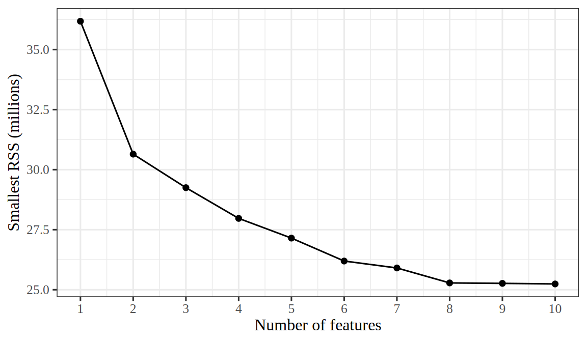
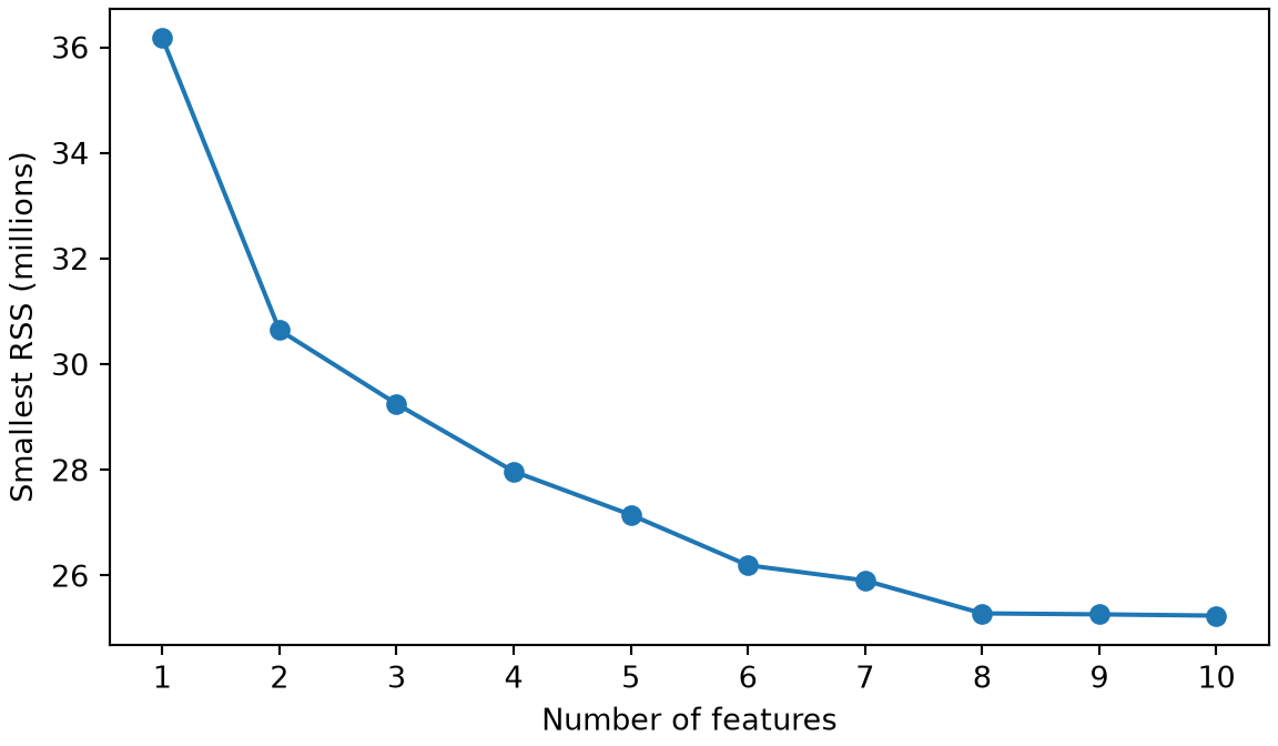
Figure 1 plots the smallest residual sum of squares of each size. It falls from 36.2 million with one feature, CRBI, to 30.6 million with two, and by a further 18% as the other eight features enter. The residual sum of squares never rises as a feature is added, so it cannot choose the size: one of the criteria in Definition 3 chooses the size.

Show code
# Plot the smallest RSS of each size, in millions, against the size.
bs_best |>
  dplyr::mutate(rss_millions = rss / 1e6) |>
  ggplot2::ggplot() +
  ggplot2::aes(x = size, y = rss_millions) +
  ggplot2::geom_line() +
  ggplot2::geom_point() +
  ggplot2::scale_x_continuous(breaks = 1:10) +
  ggplot2::labs(x = "Number of features", y = "Smallest RSS (millions)")
Show code
import matplotlib.pyplot as plt

# Plot the smallest RSS of each size, in millions, against the size.
fig, ax = plt.subplots(figsize=(6, 3.5), layout="constrained")
ax.plot(bs_best["size"], bs_best["rss"] / 1e6, marker="o");
ax.set_xticks(bs_best["size"]);
ax.set_xlabel("Number of features");
ax.set_ylabel("Smallest RSS (millions)");
plt.show()
Figure 1: The smallest residual sum of squares among the least-squares models of Salary with each number of the ten candidate features, from best subset selection on the Hitters data.
(a)
Line plot of the smallest RSS of each size, 1 to 10 features. It falls steeply from about 36 million with one feature to about 31 million with two, then slowly, to about 25 million with ten.
(b)
Line plot of the smallest RSS of each size, 1 to 10 features. It falls steeply from about 36 million with one feature to about 31 million with two, then slowly, to about 25 million with ten.
ExrExercise 4 (Choosing the size of the best subset by Mallows’ \(C_p\))

Exercise 4 (Choosing the size of the best subset by Mallows’ \(C_p\)) Best subset selection keeps one model of each size, and the residual sum of squares cannot choose among them, because it never rises as a feature enters. A criterion that adds a penalty for each feature can choose. Example 3 keeps the best subsets of the ten candidate features for the Salary of the players in the Hitters data, one for each number of features \(\subsetsize\) from \(1\) to \(10\). Estimate the noise variance by the residual variance of the model with all ten features.

TipHint

Mallows’ \(C_p\) adds \(2 \est{\varpar}\) to the \(\RSS\) for each feature. bs_best in Example 3 holds the smallest \(\RSS\) of each size.

Which \(\subsetsize\) gives the smallest Mallows’ \(C_p\)?

Solution 4.

Show code
# Estimate the noise variance from the model with all ten features,
# then add 2 * sigma2 per feature to each size's smallest RSS.
bs_n <- nrow(bs_hitters)
bs_full_rss <- bs_best$rss[10]
bs_sigma2 <- bs_full_rss / (bs_n - 10 - 1)
bs_criteria <- bs_best |>
  dplyr::select(size, rss) |>
  dplyr::mutate(cp = (rss + 2 * size * bs_sigma2) / bs_n)
bs_cp_size <- bs_criteria$size[which.min(bs_criteria$cp)]
bs_criteria
Show code
# Estimate the noise variance from the model with all ten features,
# then add 2 * sigma2 per feature to each size's smallest RSS.
bs_n = len(bs_hitters)
bs_sigma2 = bs_best["rss"].iloc[9] / (bs_n - 10 - 1)
bs_criteria = bs_best[["size", "rss"]].copy()
bs_criteria["cp"] = (bs_criteria["rss"] + 2 * bs_criteria["size"] * bs_sigma2) / bs_n
print(bs_criteria.to_string())
   size           rss             cp
0     1  3.617968e+07  138327.012419
1     2  3.064656e+07  118050.227806
2     3  2.924930e+07  113499.132660
3     4  2.797085e+07  109399.816961
4     5  2.714990e+07  107040.017066
5     6  2.619490e+07  104170.547510
6     7  2.590655e+07  103835.827298
7     8  2.528358e+07  102228.810630
8     9  2.526507e+07  102920.114893
9    10  2.524095e+07  103590.119885
Show code
# Plot Cp against the number of features, and mark the smallest value in red.
bs_cp_best <- bs_criteria |> dplyr::filter(size == bs_cp_size)
bs_criteria |>
  ggplot2::ggplot() +
  ggplot2::aes(x = size, y = cp / 1e3) +
  ggplot2::geom_line() +
  ggplot2::geom_point() +
  ggplot2::geom_point(data = bs_cp_best, colour = "red", size = 3) +
  ggplot2::scale_x_continuous(
    breaks = 1:10 # check-unexplained-choices: allow
  ) +
  ggplot2::labs(x = "Number of features", y = "Mallows' Cp (thousands)")
Show code
import matplotlib.pyplot as plt

# Plot Cp against the number of features, and mark the smallest value in red.
bs_cp_best = bs_criteria.loc[bs_criteria["cp"].idxmin()]
fig, ax = plt.subplots(figsize=(6, 3.5), layout="constrained")
ax.plot(bs_criteria["size"], bs_criteria["cp"] / 1e3, marker="o");
ax.plot(bs_cp_best["size"], bs_cp_best["cp"] / 1e3, "o", color="red", markersize=9);
ax.set_xticks(bs_criteria["size"]);
ax.set_xlabel("Number of features");
ax.set_ylabel("Mallows' Cp (thousands)");
plt.show()
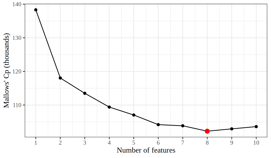
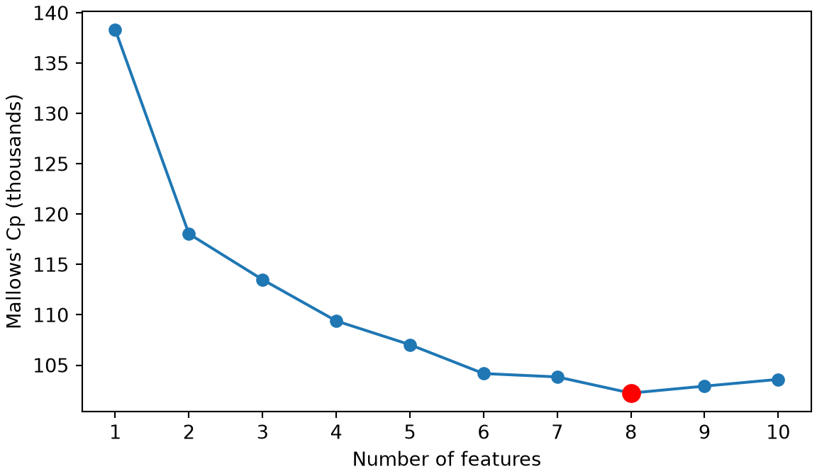
Figure 2: Mallows’ \(C_p\) of the best subset model of each size for the Hitters salaries. The red point marks the smallest value.
(a)
Line plot of Mallows' Cp, in thousands, against the number of features from 1 to 10. It falls steeply from 1 to 2 features, then more slowly to a minimum, marked by a red point, and rises slightly after it.
(b)
Line plot of Mallows' Cp, in thousands, against the number of features from 1 to 10. It falls steeply from 1 to 2 features, then more slowly to a minimum, marked by a red point, and rises slightly after it.

Figure 2 shows that the model with \(\subsetsize = 8\) features, AtBat, Hits, Walks, CAtBat, CHits, CHmRun, DivisionW, PutOuts, has the smallest Mallows’ \(C_p\). Past that size, the penalty \(2 \est{\varpar}\) for each added feature exceeds the drop in the residual sum of squares.

ExrExercise 5 (Choosing the size of the best subset by the BIC)

Exercise 5 (Choosing the size of the best subset by the BIC) Use the ten best subset models of the Hitters salaries from Example 3, one for each number of features \(\subsetsize\) from \(1\) to \(10\). Treat each of these models as a Gaussian linear model, whose \(\subsetsize\) slopes, intercept and noise variance are \(\subsetsize + 2\) estimated parameters.

TipHint

The BIC needs the maximized log-likelihood. For a Gaussian linear model fitted by least squares to \(\nobs\) observations, it is \(-\frac{\nobs}{2} \paren{\logf{2 \pi \RSS / \nobs} + 1}\). In R, stats::BIC() of the lm() fit gives the same value.

Which \(\subsetsize\) gives the smallest BIC?

Solution 5.

Show code
# The maximized Gaussian log-likelihood of each size's best model,
# and the BIC with d + 2 estimated parameters.
bs_criteria <- bs_criteria |>
  dplyr::mutate(
    loglik = -bs_n / 2 * (log(2 * pi * rss / bs_n) + 1),
    bic = -2 * loglik + (size + 2) * log(bs_n)
  )
bs_bic_size <- bs_criteria$size[which.min(bs_criteria$bic)]
bs_criteria |> dplyr::select(size, rss, bic)
Show code
# The maximized Gaussian log-likelihood of each size's best model,
# and the BIC with d + 2 estimated parameters.
bs_criteria["loglik"] = -bs_n / 2 * (np.log(2 * np.pi * bs_criteria["rss"] / bs_n) + 1)
bs_criteria["bic"] = -2 * bs_criteria["loglik"] + (bs_criteria["size"] + 2) * np.log(bs_n)
print(bs_criteria[["size", "rss", "bic"]].to_string())
   size           rss          bic
0     1  3.617968e+07  3874.855770
1     2  3.064656e+07  3836.775921
2     3  2.924930e+07  3830.075210
3     4  2.797085e+07  3823.893218
4     5  2.714990e+07  3821.630702
5     6  2.619490e+07  3817.785232
6     7  2.590655e+07  3820.446200
7     8  2.528358e+07  3819.616756
8     9  2.526507e+07  3824.996277
9    10  2.524095e+07  3830.317297
Show code
# Plot the BIC against the number of features; mark the smallest in red.
bs_bic_best <- bs_criteria |> dplyr::filter(size == bs_bic_size)
bs_criteria |>
  ggplot2::ggplot() +
  ggplot2::aes(x = size, y = bic) +
  ggplot2::geom_line() +
  ggplot2::geom_point() +
  ggplot2::geom_point(data = bs_bic_best, colour = "red", size = 3) +
  ggplot2::scale_x_continuous(
    breaks = 1:10 # check-unexplained-choices: allow
  ) +
  ggplot2::labs(x = "Number of features", y = "BIC")
Show code
# Plot the BIC against the number of features; mark the smallest in red.
bs_bic_best = bs_criteria.loc[bs_criteria["bic"].idxmin()]
fig, ax = plt.subplots(figsize=(6, 3.5), layout="constrained")
ax.plot(bs_criteria["size"], bs_criteria["bic"], marker="o");
ax.plot(bs_bic_best["size"], bs_bic_best["bic"], "o", color="red", markersize=9);
ax.set_xticks(bs_criteria["size"]);
ax.set_xlabel("Number of features");
ax.set_ylabel("BIC");
plt.show()
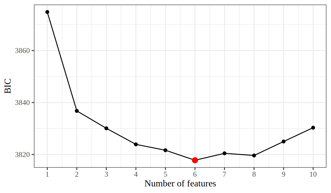
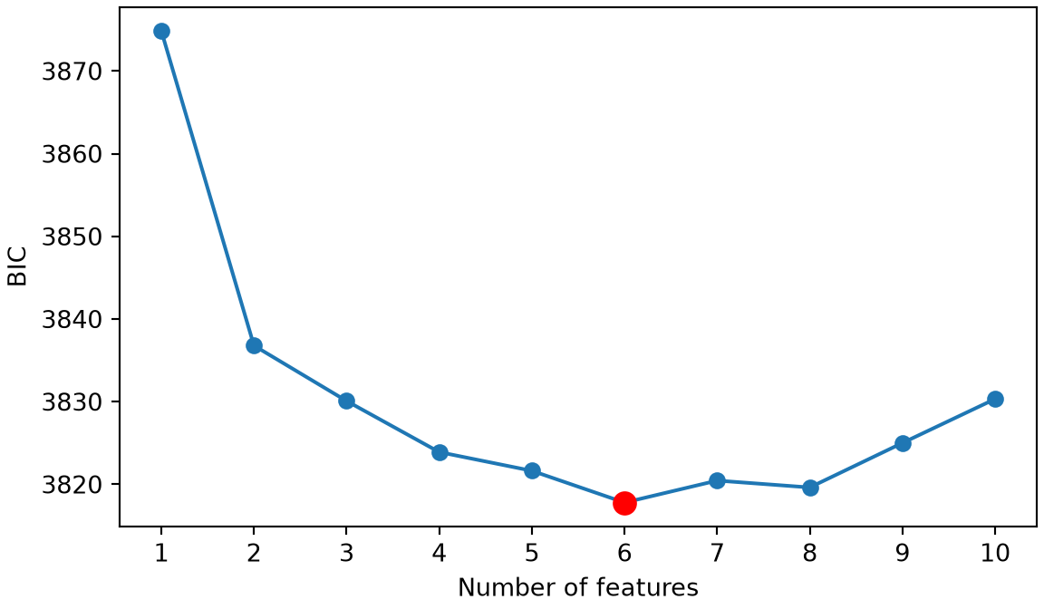
Figure 3: The BIC of the best subset model of each size for the Hitters salaries. The red point marks the smallest value.
(a)
Line plot of the BIC against the number of features from 1 to 10. It falls steeply from 1 to 2 features, reaches a minimum, marked by a red point, and then rises as more features enter.
(b)
Line plot of the BIC against the number of features from 1 to 10. It falls steeply from 1 to 2 features, reaches a minimum, marked by a red point, and then rises as more features enter.

Figure 3 shows that the model with \(\subsetsize = 6\) features, AtBat, Hits, Walks, CRBI, DivisionW, PutOuts, has the smallest BIC. The BIC charges \(\logf{\nobs} = 5.57\) for each parameter, more than the charge of \(2\) that the AIC makes. In Exercise 4, Mallows’ \(C_p\) chooses \(\subsetsize = 8\), and here the BIC chooses \(\subsetsize = 6\).

ExrExercise 6 (Choosing the size of the best subset by the adjusted \(R^2\))

Exercise 6 (Choosing the size of the best subset by the adjusted \(R^2\)) Use the ten best subset models of the Hitters salaries from Example 3, one for each number of features \(\subsetsize\) from \(1\) to \(10\).

TipHint

The adjusted \(R^2\) divides the \(\RSS\) by \(\nobs - \subsetsize - 1\) and the total sum of squares \(\TSS\) by \(\nobs - 1\), so it needs the \(\TSS\) of Salary as well as bs_best.

Which \(\subsetsize\) gives the largest adjusted \(R^2\)?

Solution 6.

Show code
# The total sum of squares of Salary, and each best model's adjusted R^2.
bs_salary_dev <- bs_hitters$Salary - mean(bs_hitters$Salary)
bs_tss <- sum(bs_salary_dev^2)
bs_criteria <- bs_criteria |>
  dplyr::mutate(adj_r2 = 1 - (rss / (bs_n - size - 1)) / (bs_tss / (bs_n - 1)))
bs_adjr2_size <- bs_criteria$size[which.max(bs_criteria$adj_r2)]
bs_criteria |> dplyr::select(size, rss, adj_r2)
Show code
# The total sum of squares of Salary, and each best model's adjusted R^2.
bs_tss = ((bs_y - bs_y.mean()) ** 2).sum()
bs_criteria["adj_r2"] = 1 - (bs_criteria["rss"] / (bs_n - bs_criteria["size"] - 1)) / (bs_tss / (bs_n - 1))
print(bs_criteria[["size", "rss", "adj_r2"]].to_string())
   size           rss    adj_r2
0     1  3.617968e+07  0.318850
1     2  3.064656e+07  0.420802
2     3  2.924930e+07  0.445075
3     4  2.797085e+07  0.467273
4     5  2.714990e+07  0.480897
5     6  2.619490e+07  0.497200
6     7  2.590655e+07  0.500785
7     8  2.528358e+07  0.510871
8     9  2.526507e+07  0.509297
9    10  2.524095e+07  0.507820
Show code
# Plot the adjusted R^2 against the size; mark the largest in red.
bs_adjr2_best <- bs_criteria |> dplyr::filter(size == bs_adjr2_size)
bs_criteria |>
  ggplot2::ggplot() +
  ggplot2::aes(x = size, y = adj_r2) +
  ggplot2::geom_line() +
  ggplot2::geom_point() +
  ggplot2::geom_point(data = bs_adjr2_best, colour = "red", size = 3) +
  ggplot2::scale_x_continuous(
    breaks = 1:10 # check-unexplained-choices: allow
  ) +
  ggplot2::labs(x = "Number of features", y = "Adjusted R-squared")
Show code
# Plot the adjusted R^2 against the size; mark the largest in red.
bs_adjr2_best = bs_criteria.loc[bs_criteria["adj_r2"].idxmax()]
fig, ax = plt.subplots(figsize=(6, 3.5), layout="constrained")
ax.plot(bs_criteria["size"], bs_criteria["adj_r2"], marker="o");
ax.plot(bs_adjr2_best["size"], bs_adjr2_best["adj_r2"], "o", color="red", markersize=9);
ax.set_xticks(bs_criteria["size"]);
ax.set_xlabel("Number of features");
ax.set_ylabel("Adjusted R-squared");
plt.show()
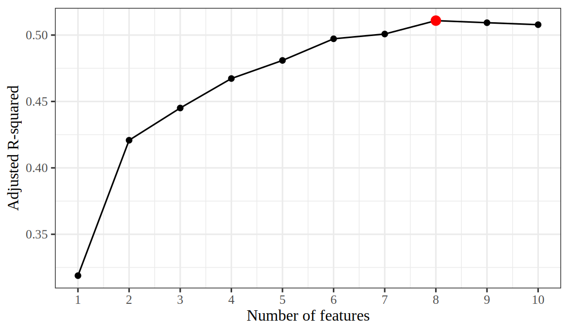
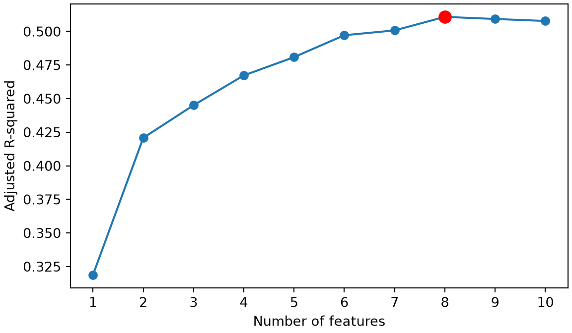
Figure 4: The adjusted \(R^2\) of the best subset model of each size for the Hitters salaries. The red dot marks the largest value.
(a)
Line plot of the adjusted R-squared against the number of features from 1 to 10. It rises steeply from 1 to 2 features, then slowly to a maximum, marked by a red dot, and levels off after it.
(b)
Line plot of the adjusted R-squared against the number of features from 1 to 10. It rises steeply from 1 to 2 features, then slowly to a maximum, marked by a red dot, and levels off after it.

Figure 4 shows that the model with \(\subsetsize = 8\) features, AtBat, Hits, Walks, CAtBat, CHits, CHmRun, DivisionW, PutOuts, has the largest adjusted \(R^2\). Mallows’ \(C_p\) chooses \(\subsetsize = 8\), the BIC chooses \(\subsetsize = 6\), and the adjusted \(R^2\) chooses \(\subsetsize = 8\). The book’s lab, with all nineteen candidate features, also finds the BIC choosing the smallest model of the three [2, Sec. 6.5.1].

PrpProposition 1 (Number of models that best subset selection fits)

Proposition 1 (Number of models that best subset selection fits) Best subset selection over \(\ninputvars\) candidate features fits \(2^{\ninputvars}\) models.

Proof. Best subset selection fits one model for each subset of the \(\ninputvars\) candidate features. A subset is fixed by choosing, for each feature, whether it is in or out: \(\ninputvars\) choices of two options each, so there are \(2^{\ninputvars}\) subsets, as Solution 1 found.

ExmExample 4 (Counting the fits on baseball salaries)

Example 4 (Counting the fits on baseball salaries) Best subset selection on the ten candidate features of Example 3 fits 1023 models with at least one feature, and one model with no features: 1024 models in all, which is \(2^{10}\), as Proposition 1 states.

ExrExercise 7 (Where forward selection misses the best subset)

Exercise 7 (Where forward selection misses the best subset) Use the Hitters data and the ten candidate features for Salary of Example 3. Run forward selection over the same candidates, on all the players, scoring each step by the residual sum of squares.

TipHint

Example 1 codes forward selection on the Auto data, and bs_rss() in Example 3 scores a list of features.

State the numbers of features at which forward selection’s model differs from the best subset model of the same size.

Solution 7.

Show code
# Forward selection: at each step, add the feature that lowers the RSS most.
bs_forward <- character(0)
bs_forward_rss <- numeric(0)
bs_remaining <- bs_candidates
rss_type <- numeric(1)
has_remaining <- TRUE
while (has_remaining) {
  scores <- vapply(bs_remaining, \(f) {
    trial <- c(bs_forward, f)
    bs_rss(trial)
  }, rss_type)
  best <- which.min(scores)
  bs_forward <- c(bs_forward, bs_remaining[best])
  bs_forward_rss <- c(bs_forward_rss, scores[best])
  bs_remaining <- bs_remaining[-best]
  has_remaining <- length(bs_remaining) > 0
}

# Forward selection's model of size k holds the first k features to enter.
# It differs from the best subset of size k when its RSS is larger.
bs_compare <- bs_best |>
  dplyr::mutate(forward_rss = bs_forward_rss,
                differs = forward_rss > rss * (1 + 1e-9))
bs_differ <- bs_compare |> dplyr::filter(differs)
bs_differ |>
  dplyr::select(size, features, rss, forward_rss)
Show code
bs_forward
 [1] "CRBI"      "Hits"      "PutOuts"   "DivisionW" "AtBat"     "Walks"    
 [7] "CRuns"     "CAtBat"    "CHits"     "CHmRun"   
Show code
# Forward selection: at each step, add the feature that lowers the RSS most.
bs_forward, bs_forward_rss = [], []
bs_remaining = list(bs_candidates)
while bs_remaining:
    scores = [bs_rss(bs_forward + [f]) for f in bs_remaining]
    best = int(np.argmin(scores))
    bs_forward.append(bs_remaining.pop(best))
    bs_forward_rss.append(scores[best])

# Forward selection's model of size k holds the first k features to enter.
# It differs from the best subset of size k when its RSS is larger.
bs_compare = bs_best.assign(forward_rss=bs_forward_rss)
bs_compare["differs"] = bs_compare["forward_rss"] > bs_compare["rss"] * (1 + 1e-9)
print(bs_compare.loc[bs_compare["differs"], ["size", "features", "rss", "forward_rss"]].to_string())
   size                                                       features           rss   forward_rss
6     7         Hits, Walks, CAtBat, CHits, CHmRun, DivisionW, PutOuts  2.590655e+07  2.608421e+07
7     8  AtBat, Hits, Walks, CAtBat, CHits, CHmRun, DivisionW, PutOuts  2.528358e+07  2.567165e+07
Show code
print(bs_forward)
['CRBI', 'Hits', 'PutOuts', 'DivisionW', 'AtBat', 'Walks', 'CRuns', 'CAtBat', 'CHits', 'CHmRun']

Forward selection’s model differs from the best subset model at 7 and 8 features. With 7 features, forward selection keeps the first 7 features to enter, CRBI, Hits, PutOuts, DivisionW, AtBat, Walks, CRuns, while the best subset is Hits, Walks, CAtBat, CHits, CHmRun, DivisionW, PutOuts, with a residual sum of squares 25.91 million against forward selection’s 26.08 million. Forward selection never removes CRBI, its first feature, but the best subsets of those sizes leave it out, so forward selection cannot reach them. At every other size the two methods agree. The book’s lab, with all nineteen candidate features, also finds the two methods first differing at seven features [2, Sec. 6.5.1].

ExrExercise 8 (Where backward selection misses the best subset)

Exercise 8 (Where backward selection misses the best subset) Use the Hitters data and the ten candidate features for Salary of Example 3. Run backward selection over the same candidates, on all the players, scoring each step by the residual sum of squares.

TipHint

Example 2 codes backward selection on the Auto data, and Solution 7 compares forward selection with the best subset on these candidates.

State the numbers of features at which backward selection’s model differs from the best subset model of the same size.

Solution 8.

Show code
# Backward selection: start from all ten features, and at each step
# remove the feature whose removal raises the RSS least.
n_candidates <- length(bs_candidates)
bs_kept <- bs_candidates
bs_removed <- character(0)
bs_backward_rss <- numeric(n_candidates)
bs_backward_rss[n_candidates] <- bs_rss(bs_kept)
rss_type <- numeric(1)
n_kept <- n_candidates
has_more <- n_kept > 1
while (has_more) {
  scores <- vapply(bs_kept, \(f) {
    trial <- setdiff(bs_kept, f)
    bs_rss(trial)
  }, rss_type)
  worst <- which.min(scores)
  bs_removed <- c(bs_removed, bs_kept[worst])
  bs_kept <- bs_kept[-worst]
  n_kept <- length(bs_kept)
  bs_backward_rss[n_kept] <- scores[worst]
  has_more <- n_kept > 1
}

# Compare the model of each size with the best subset and with
# forward selection's model (forward_rss, from the forward solution).
bs_compare_bwd <- bs_compare |>
  dplyr::mutate(
    backward_rss = bs_backward_rss,
    backward_vs_best = backward_rss > rss * (1 + 1e-9),
    backward_vs_forward = abs(backward_rss - forward_rss) > rss * 1e-9
  )
bs_compare_bwd |>
  dplyr::select(size, rss, forward_rss, backward_rss)
Show code
bs_removed
[1] "CHmRun"    "CRuns"     "AtBat"     "Hits"      "CRBI"      "DivisionW"
[7] "PutOuts"   "CAtBat"    "Walks"    
Show code
# Backward selection: start from all ten features, and at each step
# remove the feature whose removal raises the RSS least.
bs_kept = list(bs_candidates)
bs_removed = []
bs_backward_rss = {len(bs_kept): bs_rss(bs_kept)}
while len(bs_kept) > 1:
    scores = [bs_rss([g for g in bs_kept if g != f]) for f in bs_kept]
    worst = int(np.argmin(scores))
    bs_removed.append(bs_kept.pop(worst))
    bs_backward_rss[len(bs_kept)] = scores[worst]

# Compare the model of each size with the best subset and with
# forward selection's model (forward_rss, from the forward solution).
bs_compare_bwd = bs_compare.assign(backward_rss=bs_compare["size"].map(bs_backward_rss))
print(bs_compare_bwd[["size", "rss", "forward_rss", "backward_rss"]].to_string())
   size           rss   forward_rss  backward_rss
0     1  3.617968e+07  3.617968e+07  3.725397e+07
1     2  3.064656e+07  3.064656e+07  3.223904e+07
2     3  2.924930e+07  2.924930e+07  3.006368e+07
3     4  2.797085e+07  2.797085e+07  2.869575e+07
4     5  2.714990e+07  2.714990e+07  2.750693e+07
5     6  2.619490e+07  2.619490e+07  2.646897e+07
6     7  2.590655e+07  2.608421e+07  2.596912e+07
7     8  2.528358e+07  2.567165e+07  2.541457e+07
8     9  2.526507e+07  2.526507e+07  2.526507e+07
9    10  2.524095e+07  2.524095e+07  2.524095e+07
Show code
print(bs_removed)
['CHmRun', 'CRuns', 'AtBat', 'Hits', 'CRBI', 'DivisionW', 'PutOuts', 'CAtBat', 'Walks']

Backward selection’s model differs from the best subset model at every size from 1 to 8 features, and agrees with it only at 9 and 10 features. It removes CRBI at step 5, going from 6 features to 5, and never puts it back, but the best subset of every size up to 5 contains CRBI. Its model with one feature is CHits, with a residual sum of squares of 37.25 million against 36.18 million for the best single feature, CRBI.

Backward selection’s model also differs from forward selection’s at exactly those sizes, 1 to 8. At 7 and 8 features the three methods choose three different models, as the book’s lab finds at seven features with all nineteen candidates [2, Sec. 6.5.1].

4 Choosing the size by cross-validation

ExrExercise 9 (Forward selection on baseball salaries, sized by cross-validation)

Exercise 9 (Forward selection on baseball salaries, sized by cross-validation) The Hitters data hold the 1986 and career statistics of Major League baseball players, with their 1987 salaries in thousands of dollars. Drop the players whose salary is missing, and code League, Division and NewLeague as \(0/1\) indicators, which leaves \(19\) candidate features for the salary. Randomly split the players into a training half and a test half.

On the training half, run forward selection (Definition 1) with the RSS as the score, and record the order in which the features enter.

Solution 9.

hs <- na.omit(read.csv("data/hitters.csv"))
hs_x <- model.matrix(Salary ~ ., data = hs)[, -1]
hs_y <- hs$Salary

set.seed(1)
hs_train <- sample(nrow(hs), nrow(hs) / 2)
xt <- hs_x[hs_train, ]
yt <- hs_y[hs_train]

rss_of <- function(x, y, cols) {
  sum(lm.fit(cbind(1, x[, cols, drop = FALSE]), y)$residuals^2)
}

# Forward selection by the RSS: the features in the order they enter.
hs_forward <- function(x, y) {
  chosen <- integer(0)
  while (length(chosen) < ncol(x)) {
    rest <- setdiff(seq_len(ncol(x)), chosen)
    scores <- sapply(rest, function(j) rss_of(x, y, c(chosen, j)))
    chosen <- c(chosen, rest[which.min(scores)])
  }
  chosen
}

# Predictions of the model with the first `size` features of `entry`.
hs_predict <- function(x, y, entry, size, x_new) {
  cols <- entry[seq_len(size)]
  fit <- lm.fit(cbind(1, x[, cols, drop = FALSE]), y)
  drop(cbind(1, x_new[, cols, drop = FALSE]) %*% fit$coefficients)
}

entry_all <- hs_forward(xt, yt)
colnames(xt)[entry_all]
 [1] "CRBI"       "Walks"      "DivisionW"  "Years"      "PutOuts"   
 [6] "CHits"      "CAtBat"     "LeagueN"    "CHmRun"     "Assists"   
[11] "AtBat"      "HmRun"      "NewLeagueN" "Errors"     "CRuns"     
[16] "CWalks"     "Hits"       "Runs"       "RBI"       
hs_py = pd.read_csv("data/hitters.csv").dropna()
hs_x = pd.get_dummies(hs_py.drop(columns="Salary"), drop_first=True)
hs_names = list(hs_x.columns)
hs_x = hs_x.to_numpy(dtype=float)
hs_y = hs_py["Salary"].to_numpy()

hs_rng = np.random.default_rng(1)
hs_train = hs_rng.permutation(len(hs_y))[: len(hs_y) // 2]
hs_test = np.setdiff1d(np.arange(len(hs_y)), hs_train)
xt = hs_x[hs_train]
yt = hs_y[hs_train]

def hs_design(x, cols):
    return np.column_stack([np.ones(len(x)), x[:, cols]])

def hs_beta(x, y, cols):
    return np.linalg.lstsq(hs_design(x, cols), y, rcond=None)[0]

def hs_rss(x, y, cols):
    r = y - hs_design(x, cols) @ hs_beta(x, y, cols)
    return r @ r

# Forward selection by the RSS: the features in the order they enter.
def hs_forward_py(x, y):
    chosen = []
    while len(chosen) < x.shape[1]:
        rest = [j for j in range(x.shape[1]) if j not in chosen]
        chosen.append(min(rest, key=lambda j: hs_rss(x, y, chosen + [j])))
    return chosen

# Predictions of the model with the first `size` features of `entry`.
def hs_predict_py(x, y, entry, size, x_new):
    cols = entry[:size]
    return hs_design(x_new, cols) @ hs_beta(x, y, cols)

entry_all_py = hs_forward_py(xt, yt)
[hs_names[j] for j in entry_all_py]
['CRBI', 'Hits', 'Division_W', 'AtBat', 'PutOuts', 'Years', 'Assists', 'Walks', 'CWalks', 'League_N', 'CRuns', 'CAtBat', 'NewLeague_N', 'Runs', 'CHits', 'Errors', 'CHmRun', 'RBI', 'HmRun']

1. The two languages split the players at random in different ways, so their numbers differ. The numbers below are from the R split.

On the training half, the features enter in the order CRBI, Walks, DivisionW, Years, PutOuts, and so on.

ExrExercise 10 (Forward selection on baseball salaries, sized by cross-validation (part 2))

Exercise 10 (Forward selection on baseball salaries, sized by cross-validation (part 2)) Use the setup of Exercise 9.

Randomly assign the training players to ten folds. For each size \(\subsetsize = 1, \dots, 19\), compute the 10-fold cross-validation root mean squared error (RMSE) of the model that has the first \(\subsetsize\) features chosen by forward selection. Run the forward selection again on the other nine folds of each split.

Solution 10.

# The selection is repeated on the other nine folds of each split.
set.seed(2)
folds <- sample(rep(1:10, length.out = nrow(xt)))
cv_sq <- matrix(NA_real_, nrow(xt), ncol(xt))
for (f in 1:10) {
  held <- folds == f
  entry_f <- hs_forward(xt[!held, ], yt[!held])
  for (m in seq_len(ncol(xt))) {
    pred <- hs_predict(xt[!held, ], yt[!held], entry_f, m, xt[held, , drop = FALSE])
    cv_sq[held, m] <- (yt[held] - pred)^2
  }
}
cv_rmse <- sqrt(colMeans(cv_sq))
m_best <- which.min(cv_rmse)
data.frame(size = seq_along(cv_rmse), cv_rmse = round(cv_rmse))
# The selection is repeated on the other nine folds of each split.
folds_py = np.random.default_rng(2).permutation(np.arange(len(yt)) % 10)
cv_sq_py = np.empty((len(yt), xt.shape[1]))
for f in range(10):
    held = folds_py == f
    entry_f = hs_forward_py(xt[~held], yt[~held])
    for m in range(1, xt.shape[1] + 1):
        pred = hs_predict_py(xt[~held], yt[~held], entry_f, m, xt[held])
        cv_sq_py[held, m - 1] = (yt[held] - pred) ** 2
cv_rmse_py = np.sqrt(cv_sq_py.mean(axis=0))
m_best_py = int(np.argmin(cv_rmse_py)) + 1
print(pd.DataFrame({"size": range(1, xt.shape[1] + 1), "cv_rmse": cv_rmse_py.round()}))
    size  cv_rmse
0      1    409.0
1      2    420.0
2      3    400.0
3      4    390.0
4      5    383.0
5      6    385.0
6      7    376.0
7      8    392.0
8      9    395.0
9     10    390.0
10    11    376.0
11    12    376.0
12    13    373.0
13    14    372.0
14    15    374.0
15    16    378.0
16    17    378.0
17    18    378.0
18    19    378.0

2. Cross-validation chooses \(\subsetsize =\) 3 features, with a cross-validation RMSE of 320 thousand dollars.

ExrExercise 11 (Forward selection on baseball salaries, sized by cross-validation (part 3))

Exercise 11 (Forward selection on baseball salaries, sized by cross-validation (part 3)) Use the setup of Exercise 9.

Choose the size \(\subsetsize\) with the smallest cross-validation RMSE, refit that model on the whole training half, and compute its root mean squared error on the test half.

Solution 11.

test_rmse_of <- function(m) {
  pred <- hs_predict(xt, yt, entry_all, m, hs_x[-hs_train, ])
  sqrt(mean((hs_y[-hs_train] - pred)^2))
}
c(chosen = test_rmse_of(m_best), all = test_rmse_of(ncol(xt)))
  chosen      all 
389.6647 410.6011 
def hs_test_rmse(m):
    pred = hs_predict_py(xt, yt, entry_all_py, m, hs_x[hs_test])
    return float(np.sqrt(np.mean((hs_y[hs_test] - pred) ** 2)))

print("chosen size", m_best_py, "- test RMSE", round(hs_test_rmse(m_best_py)),
      "- all features", round(hs_test_rmse(xt.shape[1])))
chosen size 14 - test RMSE 332 - all features 332

The model that cross-validation chooses has a test RMSE of 390 thousand dollars on the test half.

ExrExercise 12 (Forward selection on baseball salaries, sized by cross-validation (part 4))

Exercise 12 (Forward selection on baseball salaries, sized by cross-validation (part 4)) Use the setup of Exercise 9.

Compare it with the test error of the model that uses all \(19\) features.

Solution 12. The model with all 19 features has a test RMSE of 411 thousand dollars, which is higher than the test RMSE of the model that cross-validation chooses.

ExrExercise 13 (Forward selection on baseball salaries, sized by cross-validation (part 5))

Exercise 13 (Forward selection on baseball salaries, sized by cross-validation (part 5)) Use the setup of Exercise 9.

Why must the forward selection be run again inside each split, rather than once on the whole training half?

Solution 13. 4. The selection is repeated inside each split because the features chosen on the whole training half have already seen every training player’s salary. The held-out fold would then not be new data for the selection, and the cross-validation error would be too small.

ExrExercise 14 (Forward selection on baseball salaries, sized by cross-validation (part 6))

Exercise 14 (Forward selection on baseball salaries, sized by cross-validation (part 6)) Use the training half of the Hitters players, its ten folds, and the held-out squared errors of each size from Exercise 10.

A cross-validation estimate depends on which players land in which fold, so another assignment of players to folds would give a different value for each size. Two sizes whose values differ by less than that variation may give about equally good predictions, and the smaller of them has fewer features to record and interpret.

Plot the cross-validation estimate of the mean squared error of each size against the size, with a bar of one fold-based standard error on each side.

The fold-based standard error is the sample standard deviation of the ten fold mean squared errors, divided by \(\sqrt{10}\). Compute the fold mean squared errors of each size from the held-out squared errors of the players in each fold.

Solution 14.

Show code
# The cross-validation estimate of each size pools the held-out squared errors.
cv_est <- colMeans(cv_sq)

# The fold mean squared errors: one row per fold, one column per size.
fold_sums <- rowsum(cv_sq, folds)
fold_counts <- tabulate(folds)
fold_mse <- fold_sums / fold_counts

# The fold-based standard error of each size.
fold_sd <- apply(fold_mse, 2, sd)
cv_se <- fold_sd / sqrt(10)

# The spread of the estimates, to compare with the SE at the minimum.
cv_spread <- max(cv_est) - min(cv_est)
se_at_min <- cv_se[which.min(cv_est)]

cv_sizes <- seq_along(cv_est)
cv_tbl <- tibble::tibble(size = cv_sizes, estimate = cv_est, se = cv_se)
cv_tbl
Show code
# The cross-validation estimate of each size pools the held-out squared errors.
cv_est_py = cv_sq_py.mean(axis=0)

# The fold mean squared errors: one row per fold, one column per size.
fold_mse_py = np.array([cv_sq_py[folds_py == f].mean(axis=0) for f in range(10)])

# The fold-based standard error of each size.
cv_se_py = fold_mse_py.std(axis=0, ddof=1) / np.sqrt(10)

cv_tbl_py = pd.DataFrame({"size": range(1, xt.shape[1] + 1),
                          "estimate": cv_est_py, "se": cv_se_py})
print(cv_tbl_py.round().to_string(index=False))
 size  estimate      se
    1  167379.0 39539.0
    2  176630.0 42095.0
    3  160313.0 39971.0
    4  151756.0 36592.0
    5  146871.0 35102.0
    6  148335.0 35090.0
    7  141246.0 33944.0
    8  153465.0 36330.0
    9  155847.0 37679.0
   10  152185.0 37286.0
   11  141083.0 36026.0
   12  141252.0 37870.0
   13  138768.0 37151.0
   14  138738.0 37489.0
   15  139716.0 37867.0
   16  142965.0 40121.0
   17  142777.0 39505.0
   18  142735.0 39502.0
   19  142957.0 39465.0
Show code
# Plot each size's estimate with a bar of one standard error on each side.
cv_tbl |>
  ggplot2::ggplot() +
  ggplot2::aes(x = size, y = estimate / 1e3) +
  ggplot2::geom_linerange(
    ggplot2::aes(ymin = (estimate - se) / 1e3, ymax = (estimate + se) / 1e3),
    colour = "grey50"
  ) +
  ggplot2::geom_line() +
  ggplot2::geom_point() +
  ggplot2::labs(
    x = "Number of features",
    y = "CV estimate of MSE (thousands)"
  )
Show code
# Plot each size's estimate with a bar of one standard error on each side.
fig, ax = plt.subplots(figsize=(6, 3.5), layout="constrained")
ax.errorbar(cv_tbl_py["size"], cv_tbl_py["estimate"] / 1e3,
            yerr=cv_tbl_py["se"] / 1e3, marker="o", color="black",
            ecolor="grey");
ax.set_xlabel("Number of features");
ax.set_ylabel("CV estimate of MSE (thousands)");
plt.show()
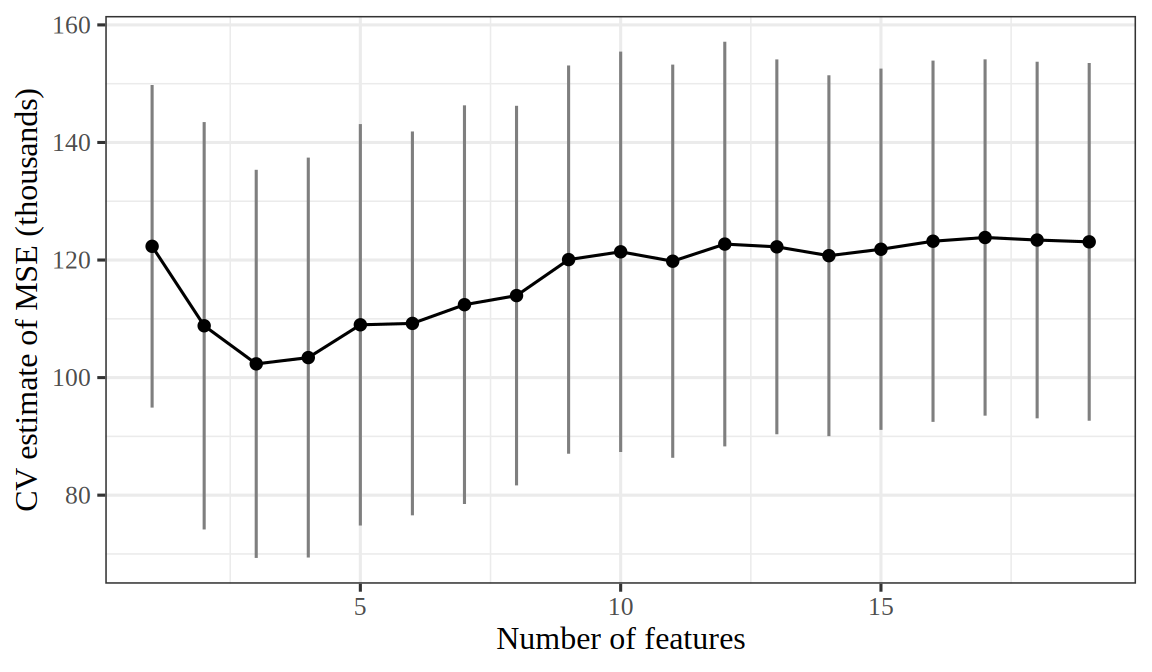
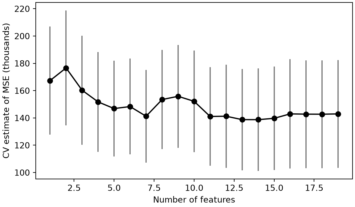
Figure 5: Cross-validation estimates of the mean squared error of the forward selection model of each size on the Hitters training half, with bars of one fold-based standard error on each side.
(a)
Cross-validation estimates of the mean squared error of forward selection on the Hitters training half, in thousands of squared thousand dollars, against the number of features from 1 to 19, each with a vertical bar of one fold-based standard error on each side. The estimates fall over the first few sizes and change little after, and the bars are wide compared with the differences between sizes.
(b)
Cross-validation estimates of the mean squared error of forward selection on the Hitters training half, in thousands of squared thousand dollars, against the number of features from 1 to 19, each with a vertical bar of one fold-based standard error on each side. The estimates fall over the first few sizes and change little after, and the bars are wide compared with the differences between sizes.

Figure 5 shows the cross-validation estimates from the R split. The smallest is at 3 features, 102 thousand, with a fold-based standard error of 33 thousand. The other sizes give values from 103 to 124 thousand. The values of all sizes lie within 21 thousand of each other, less than that fold-based standard error.

ExrExercise 15 (Forward selection on baseball salaries, sized by cross-validation (part 7))

Exercise 15 (Forward selection on baseball salaries, sized by cross-validation (part 7)) Use the cross-validation estimates and fold-based standard errors of each size from Exercise 14.

Which size does the one-standard-error rule choose?

A model of a smaller size is less flexible than one of a larger size, so the rule looks for the smallest size whose estimate is at most the smallest estimate plus that estimate’s standard error.

Solution 15.

Show code
# The cutoff is the smallest estimate plus its own standard error.
size_min <- which.min(cv_est)
cv_cutoff <- cv_est[size_min] + cv_se[size_min]

# The rule takes the smallest size whose estimate is within the cutoff.
sizes_within <- which(cv_est <= cv_cutoff)
size_one_se <- min(sizes_within)
c(smallest_estimate = size_min, one_se_rule = size_one_se)
smallest_estimate       one_se_rule 
                3                 1 
Show code
# The cutoff is the smallest estimate plus its own standard error.
size_min_py = int(np.argmin(cv_est_py)) + 1
cv_cutoff_py = cv_est_py[size_min_py - 1] + cv_se_py[size_min_py - 1]

# The rule takes the smallest size whose estimate is within the cutoff.
size_one_se_py = int(np.flatnonzero(cv_est_py <= cv_cutoff_py).min()) + 1
print("smallest estimate", size_min_py, "- one-standard-error rule", size_one_se_py)
smallest estimate 14 - one-standard-error rule 1

The one-standard-error rule chooses size 1 on the R split, whose feature is CRBI. That size is the smallest whose cross-validation estimate is at most 135 thousand, the smallest value (at 3 features) plus its fold-based standard error [2, Sec. 6.1.3].

ExrExercise 16 (Forward selection on baseball salaries, sized by cross-validation (part 8))

Exercise 16 (Forward selection on baseball salaries, sized by cross-validation (part 8)) Use the size that the one-standard-error rule chooses in Exercise 15, and the test half of the Hitters players from Exercise 9.

Compare the root mean squared error on the test half of the model of that size with the test RMSE of the model of Exercise 11, which has the size with the smallest cross-validation estimate.

Refit the model of the chosen size on the whole training half, as Exercise 11 does for its size.

Solution 16.

Show code
# Test RMSE of each choice of size, refit on the whole training half.
test_rmse_one_se <- test_rmse_of(size_one_se)
test_rmse_min <- test_rmse_of(m_best)
c(one_se_rule = test_rmse_one_se, smallest_estimate = test_rmse_min)
      one_se_rule smallest_estimate 
         432.1068          389.6647 
Show code
# Test RMSE of each choice of size, refit on the whole training half.
print("one-standard-error rule", round(hs_test_rmse(size_one_se_py)),
      "- smallest estimate", round(hs_test_rmse(m_best_py)))
one-standard-error rule 371 - smallest estimate 332

On the R split, the model of size 1 that the one-standard-error rule chooses has a test RMSE of 432 thousand dollars. The model of size 3 from Exercise 11 has a test RMSE of 390 thousand dollars. The smaller model’s test RMSE is higher by 42 thousand dollars, with 2 fewer features.

This exercise follows the subset selection lab of [2, Sec. 6.5.1], which uses the same Hitters data. The R lab picks the size of the model with regsubsets, and the Python lab uses a search from the ISLP package [4]. Here we write the forward selection of this chapter ourselves, and we choose the size by cross-validation.

5 The book’s lab

This section works through the part of the book’s Chapter 6 lab on subset selection [1, Sec. 6.5.1]. The methods in it predict an outcome from only some of the available variables, which reduces the number of coefficients the model has to fit.

Our prompts and solution text paraphrase [1, Sec. 6.5.1]. The Python code is adapted from the book’s Chapter 6 lab notebook [4], with pandas and statsmodels in place of the ISLP package. The R code is our own. Emil Hvitfeldt’s tidymodels version of the lab leaves out this part, because tidymodels supports neither best subset nor stepwise selection, so these exercises have no tidymodels tab.

ExrExercise 17 (Loading the baseball salaries)

Exercise 17 (Loading the baseball salaries) The rest of this lab predicts a player’s Salary in the Hitters data from that player’s batting and fielding records, first with forward selection and then with best subset selection. Some players have no recorded Salary.

Load the data and count the players whose Salary is missing.

Solution 17.

import numpy as np
import pandas as pd
from statsmodels.api import OLS
from functools import partial

# ISLP's load_data('Hitters') reads the same data as this file.
Hitters = pd.read_csv("data/hitters.csv")
# np.isnan() marks each missing salary, and sum() counts the marks.
np.isnan(Hitters['Salary']).sum()
np.int64(59)
hitters_raw <- readr::read_csv("data/hitters.csv", show_col_types = FALSE)
# is.na() marks each missing salary, and sum() counts the marks.
hitters_raw$Salary |>
  is.na() |>
  sum()
[1] 59

59 of the 322 players have no Salary.

ExrExercise 18 (Loading the baseball salaries (part 2))

Exercise 18 (Loading the baseball salaries (part 2)) Use the Hitters data of Exercise 17. Drop every player with a missing value in any variable. How many players and variables remain?

Solution 18.

# dropna() drops each row with a missing value in any column.
Hitters = Hitters.dropna();
Hitters.shape
(263, 20)
# na.omit() drops each row with a missing value in any column.
hitters <- na.omit(hitters_raw)
dim(hitters)
[1] 263  20

No variable other than Salary has a missing value, so dropping the 59 players without a salary leaves 263 players and 20 variables: Salary and 19 others.

ExrExercise 19 (A Mallows’ Cp scorer)

Exercise 19 (A Mallows’ Cp scorer) Use the Hitters players left in Exercise 18. Forward selection needs a score for each candidate model. Write a function that takes a fitted model and the data it was fit on, and returns its Mallows’ \(C_p\) (Equation 6.2 in [1, Sec. 6.1.3]). For \(\varpar\), use the estimate \(\est{\varpar}\) given by the residual variance of the linear model on all 19 other variables.

Solution 19. Mallows’ \(C_p\) is \((\RSS + 2 d \est{\varpar}) / n\) for a model with \(d\) coefficients fit on \(n\) players. A smaller \(C_p\) is better, but the Python follows scikit-learn’s convention that a larger score is better, so its scorer nCp() returns the negative of \(C_p\). Both scorers take a fitted model and the data it was fit on, and read \(d\) and \(n\) off the shape of that data.

def nCp(sigma2, estimator, X, Y):
    "Negative Cp statistic"
    n, p = X.shape
    Y_hat = estimator.predict(X)
    RSS = np.sum((Y - Y_hat)**2)
    return -(RSS + 2 * p * sigma2) / n

The estimate \(\est{\varpar}\) comes from the fit with every variable. ISLP builds the design matrix with its ModelSpec; here get_dummies() turns League, Division and NewLeague into 0/1 indicators instead.

X = pd.get_dummies(Hitters.drop(columns='Salary'), drop_first=True, dtype=float)
X.insert(0, 'intercept', 1.0)
Y = np.array(Hitters['Salary'])
sigma2 = OLS(Y,X).fit().scale

partial() fixes the sigma2 of nCp() at \(\est{\varpar}\), which leaves a scorer that takes a fit and its data.

neg_Cp = partial(nCp, sigma2)
lab_x <- model.matrix(Salary ~ ., data = hitters)
lab_y <- hitters$Salary
full_fit <- lm.fit(lab_x, lab_y)
# The residual variance: the RSS over the residual degrees of freedom.
sigma2 <- sum(full_fit$residuals^2) / full_fit$df.residual

# A lab helper, defined where the lab uses it.
# nolint start: function_location_linter.
# Mallows' Cp of `fit`, an lm.fit() of y on the columns of x,
# with the noise variance estimate sigma2.
cp_of <- function(fit, x, y, sigma2) {
  y_hat <- x %*% fit$coefficients
  rss <- sum((y - y_hat)^2)
  (rss + 2 * ncol(x) * sigma2) / nrow(x)
}
# nolint end

# Cp of the model with every variable.
cp_of(full_fit, lab_x, lab_y, sigma2)
[1] 107164.8

\(\est{\varpar}\) is 99,591, from the linear model with all 19 features and an intercept.

ExrExercise 20 (Forward selection scored by Mallows’ Cp)

Exercise 20 (Forward selection scored by Mallows’ Cp) Use the Hitters players and the \(C_p\) scorer of Exercise 19. Run forward selection from the model with only an intercept, and stop at the first step where no added variable improves the score. Run it twice: once scoring each model by its mean squared error on the data it was fit on, and once by \(C_p\). Which variables does each run keep?

Solution 20. ISLP runs this search with its Stepwise.first_peak() strategy and sklearn_selected() [4]. Here a short function does the same search, so the page needs no ISLP package.

def neg_MSE(estimator, X, Y):
    return -np.mean((Y - estimator.predict(X))**2)

# Forward selection from the intercept-only model,
# stopping when no added column raises the score.
def forward_first_peak(X, Y, scoring):
    selected = ['intercept']
    best = scoring(OLS(Y, X[selected]).fit(), X[selected], Y)
    rest = [c for c in X.columns if c not in selected]
    while rest:
        scores = {c: scoring(OLS(Y, X[selected + [c]]).fit(), X[selected + [c]], Y)
                  for c in rest}
        c_best = max(scores, key=scores.get)
        if scores[c_best] <= best:
            break
        selected.append(c_best)
        rest.remove(c_best)
        best = scores[c_best]
    return selected[1:]

hitters_MSE = forward_first_peak(X, Y, neg_MSE)
len(hitters_MSE)
19
hitters_Cp = forward_first_peak(X, Y, neg_Cp)
hitters_Cp
['CRBI', 'Hits', 'PutOuts', 'Division_W', 'AtBat', 'Walks', 'CWalks', 'CRuns', 'CAtBat', 'Assists']
# Lab helpers, defined where the lab uses them.
# nolint start: function_location_linter.
# The in-sample mean squared error of `fit`, an lm.fit() of y on x.
mse_of <- function(fit, x, y) {
  y_hat <- x %*% fit$coefficients
  mean((y - y_hat)^2)
}

# Forward selection on the columns of x from the intercept-only model
# (column 1), stopping when no added column lowers the score.
# `score` takes a fit, its columns of x and y, then any arguments in `...`.
forward_first_peak <- function(x, y, score, ...) {
  score_cols <- function(cols) {
    x_cols <- x[, cols, drop = FALSE]
    fit <- lm.fit(x_cols, y)
    score(fit, x_cols, y, ...)
  }
  chosen <- 1
  best <- score_cols(chosen)
  n_cols <- ncol(x)
  rest <- seq_len(n_cols)[-1]
  score_with <- function(j) {
    cols <- c(chosen, j)
    score_cols(cols)
  }
  one_number <- numeric(1)
  repeat {
    none_left <- length(rest) == 0
    if (none_left) {
      break
    }
    scores <- vapply(rest, score_with, one_number)
    pick <- which.min(scores)
    no_gain <- scores[pick] >= best
    if (no_gain) {
      break
    }
    best <- scores[pick]
    chosen <- c(chosen, rest[pick])
    rest <- rest[-pick]
  }
  all_names <- colnames(x)
  all_names[chosen[-1]]
}
# nolint end

forward_mse <- forward_first_peak(lab_x, lab_y, mse_of)
length(forward_mse)
[1] 19
forward_cp <- forward_first_peak(lab_x, lab_y, cp_of, sigma2 = sigma2)
forward_cp
 [1] "CRBI"      "Hits"      "PutOuts"   "DivisionW" "AtBat"     "Walks"    
 [7] "CWalks"    "CRuns"     "CAtBat"    "Assists"  

The in-sample mean squared error never rises when a variable enters, so the first run keeps all 19 variables. \(C_p\) adds \(2 \est{\varpar} / n\) for each coefficient, so the second run stops sooner, with 10 variables: CRBI, Hits, PutOuts, DivisionW, AtBat, Walks, CWalks, CRuns, CAtBat, Assists. The book’s lab also selects all 19 variables by MSE and 10 by \(C_p\) [1, Sec. 6.5.1].

ExrExercise 21 (Best subset selection along a path)

Exercise 21 (Best subset selection along a path) Use the Hitters players left in Exercise 18. Forward selection is greedy: each step adds one variable to the variables it already holds. Best subset selection instead searches, for each number of variables, for the best set of that many variables. Run best subset selection on all 19 other variables. Which variables are in the best model with two variables?

Solution 21. ISLP’s lab runs best subset selection with the l0bnb package [4]. It does not fix the number of variables. Instead, it charges a penalty \(\regpar_0\) for each nonzero coefficient, and returns a path of fits as \(\regpar_0\) shrinks. Penalizing the number of variables, rather than fixing it, matters once we cross-validate. l0bnb fits the intercept on its own, so the Python drops it from X. The R tab uses leaps::regsubsets(), which searches each size in turn.

# l0bnb still refers to np.Inf, an alias NumPy 2 removed; restore it first.
# The alias stays in place for the rest of the page's Python session.
np.Inf = np.inf
from l0bnb import fit_path

D = X.drop(columns='intercept')
X_l0 = np.asarray(D)
path = fit_path(X_l0,
                Y,
                max_nonzeros=X_l0.shape[1])
Preprocessing Data.
BnB Started.
Iteration: 1. Number of non-zeros:  1
Iteration: 2. Number of non-zeros:  2
Iteration: 3. Number of non-zeros:  2
Iteration: 4. Number of non-zeros:  2
Iteration: 5. Number of non-zeros:  3
Iteration: 6. Number of non-zeros:  3
Iteration: 7. Number of non-zeros:  4
Iteration: 8. Number of non-zeros:  9
Iteration: 9. Number of non-zeros:  9
Iteration: 10. Number of non-zeros:  9
Iteration: 11. Number of non-zeros:  9
Iteration: 12. Number of non-zeros:  9
Iteration: 13. Number of non-zeros:  9
Iteration: 14. Number of non-zeros:  9
Iteration: 15. Number of non-zeros:  9
Iteration: 16. Number of non-zeros:  9
Iteration: 17. Number of non-zeros:  9
Iteration: 18. Number of non-zeros:  17
Iteration: 19. Number of non-zeros:  19

Each fit on the path holds the coefficients as B, the intercept as B0, and the penalty as lambda_0. The fourth fit has two nonzero coefficients.

path[3]
{'B': array([0.        , 3.25484367, 0.        , 0.        , 0.        ,
       0.        , 0.        , 0.        , 0.        , 0.        ,
       0.        , 0.67775265, 0.        , 0.        , 0.        ,
       0.        , 0.        , 0.        , 0.        ]), 'B0': np.float64(-38.98216739555505), 'lambda_0': np.float64(0.011416248027450187), 'M': np.float64(0.5829861733382012), 'Time_exceeded': False}
best_two = list(D.columns[path[3]['B'] != 0])
lambda_two = round(path[3]['lambda_0'], 4)
best_two
['Hits', 'CRBI']
n_vars <- ncol(hitters) - 1
best_subsets <- leaps::regsubsets(Salary ~ ., data = hitters, nvmax = n_vars)
coef(best_subsets, 2)
(Intercept)        Hits        CRBI 
-47.9559022   3.3008446   0.6898994 

The best model with two variables uses Hits and CRBI. They are the two variables of the fourth fit on the l0bnb path, at \(\regpar_0\) = 0.0114. regsubsets() finds the same pair. A validation set or cross-validation along \(\regpar_0\) would choose among the fits on the path [1, Sec. 6.5.1].

Definitions on this page

Back to top

References

[1]
G. James, D. Witten, T. Hastie, R. Tibshirani, and J. Taylor, An introduction to statistical learning: With applications in Python. Springer, 2023. doi: 10.1007/978-3-031-38747-0.
[2]
G. James, D. Witten, T. Hastie, and R. Tibshirani, An introduction to statistical learning with applications in R, 2nd ed. Springer, 2021. Available: https://www.statlearning.com/
[3]
Wikipedia contributors, “Stepwise regression — Wikipedia, the free encyclopedia.” 2026. Available: https://en.wikipedia.org/wiki/Stepwise_regression
[4]
G. James, D. Witten, T. Hastie, R. Tibshirani, and J. Taylor, “ISLP labs: Lab notebooks for an introduction to statistical learning with applications in python.” GitHub repository, BSD 2-Clause license, 2023. Available: https://github.com/intro-stat-learning/ISLP_labs