# The Python chunks on this page import numpy, pandas, matplotlib, scipy and statsmodels;# reticulate provisions them.library(reticulate)py_require(c("numpy", "pandas", "matplotlib", "scipy", "statsmodels"))f3<-function(v)sprintf("%.3f", v)# A positive number in scientific notation, for display math: 2.4\times10^{2}.sci<-function(v){e<-floor(log10(v))m<-signif(v/10^e, 2)if(m>=10){m<-m/10e<-e+1}sprintf("%.1f\\times10^{%d}", m, e)}
Each solution shows the code in Python, in R with tidymodels, and in base R.
2 Helper functions
Every lab and example below reports 95% confidence intervals. These helpers are defined once, here, so no page depends on another page’s code. Each takes all its inputs as arguments.
import numpy as npdef bootstrap_corr_ci(a, b, B=20000, seed=571):"""95% percentile interval for the correlation of a and b. Resamples the cases with replacement B times, which mimics drawing new cases from the same population, and recomputes the correlation each time. """ rng = np.random.default_rng(seed) a, b = np.asarray(a, float), np.asarray(b, float) corr = np.empty(B)for i inrange(B): rows = rng.integers(0, len(a), len(a)) corr[i] = np.corrcoef(a[rows], b[rows])[0, 1]return np.quantile(corr, [0.025, 0.975])def bootstrap_vif_ci(features, B=20000, seed=571):"""95% percentile interval for each feature's VIF. The VIF of feature j is the jth diagonal entry of the inverse of the features' correlation matrix, which gives the same value as 1 / (1 - R^2) without a regression per feature. """ rng = np.random.default_rng(seed) F = np.asarray(features, float) vifs = np.empty((B, F.shape[1]))for b inrange(B): rows = rng.integers(0, len(F), len(F)) vifs[b] = np.diag(np.linalg.inv(np.corrcoef(F[rows], rowvar=False)))return np.quantile(vifs, [0.025, 0.975], axis=0)
Show code
# Formats an interval's endpoints for the proseci_text<-function(bounds, digits){sprintf("%.*f to %.*f", digits, bounds[[1]], digits, bounds[[2]])}# 95% percentile interval for R^2 from resampled cars.# Resampling rows with replacement mimics# drawing a new set of cars from the same population.# The refits use lm.fit directly, because 2,000 workflow fits would be slow.boot_r2_ci<-function(formula, data, n_boot=2000){set.seed(571)design<-model.matrix(formula, data)y<-model.response(model.frame(formula, data))r2<-vapply(seq_len(n_boot), \(b){rows<-sample(nrow(design), replace =TRUE)sse<-sum(lm.fit(design[rows, ], y[rows])$residuals^2)1-sse/sum((y[rows]-mean(y[rows]))^2)}, numeric(1))unname(quantile(r2, c(0.025, 0.975)))}# 95% percentile interval for the correlation of a and bboot_cor_ci<-function(a, b, n_boot=20000){set.seed(571)corr<-vapply(seq_len(n_boot), \(i){rows<-sample(length(a), replace =TRUE)cor(a[rows], b[rows])}, numeric(1))unname(quantile(corr, c(0.025, 0.975)))}# 95% percentile interval for each feature's VIF.# The VIF of feature j is the jth diagonal entry# of the inverse of the features' correlation matrix,# which gives the same value as 1 / (1 - R^2) without a regression per feature.boot_vif_ci<-function(features, n_boot=20000){set.seed(571)vifs<-vapply(seq_len(n_boot), \(b){resample<-features[sample(nrow(features), replace =TRUE), ]diag(solve(cor(resample)))}, numeric(ncol(features)))apply(vifs, 1, quantile, probs =c(0.025, 0.975))}# The 95% interval for a linear combination w'beta# of a fitted model's coefficients:# the estimate plus or minus a t quantile times its standard error,# from the coefficients' covariance matrixlincomb_ci<-function(model, w){estimate<-sum(w*coef(model))half<-qt(0.975, df.residual(model))*sqrt(drop(t(w)%*%vcov(model)%*%w))c(estimate =estimate, lower =estimate-half, upper =estimate+half)}
These exercises follow the lab of [1, Sec. 3.6], on the Boston and Carseats data, step by step. The Python code follows the book’s Chapter 3 lab notebook, which fits models with statsmodels. That notebook builds its design matrices with ModelSpec from the ISLP package; here we build them with pandas, because installing ISLP also installs PyTorch. The R tidymodels code follows the Chapter 3 lab of ISLR-tidymodels-labs.
3 Simple linear regression
ExrExercise 1 (Lab: fit a line to the Boston data)
Exercise 1 (Lab: fit a line to the Boston data) Download the Boston data from data/boston.csv and save it as data/boston.csv next to your code. It has \(506\) Boston neighborhoods from the 1970 census [2]. The copy here is the one in the Python package ISLP and the R package ISLR2. The response medv is the median home value, in thousands of dollars, and lstat is the percentage of the population with lower socioeconomic status.
import numpy as npimport pandas as pdimport statsmodels.api as sm# ISLP's load_data("Boston") reads this same file.Boston = pd.read_csv("data/boston.csv")medv = Boston["medv"]X_simple = pd.DataFrame({"intercept": np.ones(Boston.shape[0]),"lstat": Boston["lstat"]})boston_simple = sm.OLS(medv, X_simple).fit()# Each coefficient with its standard error and 95% confidence intervalprint(pd.concat([boston_simple.params, boston_simple.bse, boston_simple.conf_int()], axis=1) .set_axis(["coef", "std err", "lower", "upper"], axis=1))
library(tidymodels)boston<-read.csv("data/boston.csv")lm_spec<-linear_reg()|>set_engine("lm")tm_boston_simple<-lm_spec|>fit(medv~lstat, data =boston)# Each coefficient with its standard error and 95% confidence intervaltidy(tm_boston_simple, conf.int =TRUE)
boston<-read.csv("data/boston.csv")lm_boston_simple<-lm(medv~lstat, data =boston)# The table includes each coefficient's standard error# and 95% confidence intervalparameters::parameters(lm_boston_simple)|>parameters::print_md(digits =3)
Parameter
Coefficient
SE
95% CI
t(504)
p
(Intercept)
34.554
0.563
(33.448, 35.659)
61.415
< .001
lstat
-0.950
0.039
(-1.026, -0.874)
-24.528
< .001
The fitted line is \(\widehat{\text{medv}} =\) 34.55 \(-\) 0.95 \(\times\)lstat, with standard errors 0.563 and 0.039. The 95% confidence intervals, the estimate plus or minus a \(t\) quantile times its standard error, are 33.45 to 35.66 for the intercept and -1.026 to -0.874 for the slope. Each extra percentage point of lstat goes with a median home value about 950 dollars lower (95% confidence interval 874 to 1026 dollars lower).
ExrExercise 2 (Lab: fit a line to the Boston data (part 2))
Exercise 2 (Lab: fit a line to the Boston data (part 2)) Use the setup of Exercise 1.
Predictmedv for lstat values \(5\), \(10\) and \(15\).
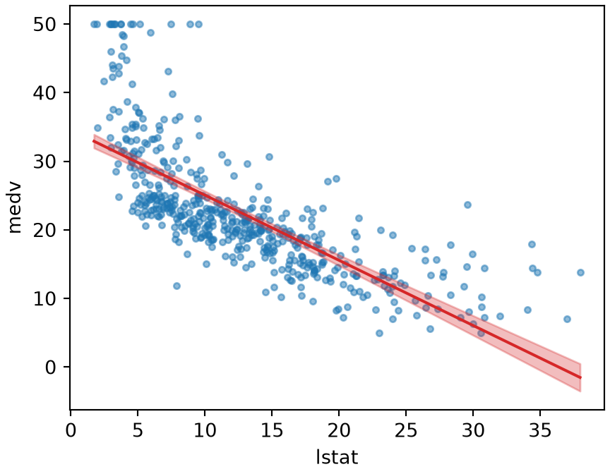
import matplotlib.pyplot as pltlstat_grid = np.linspace(Boston["lstat"].min(), Boston["lstat"].max(), 100)# The band is the 95% confidence interval for the mean medv at each lstatband = boston_simple.get_prediction( pd.DataFrame({"intercept": 1.0, "lstat": lstat_grid})).conf_int(alpha=0.05)fig, ax = plt.subplots(figsize=(4.5, 3.5), layout="constrained")ax.scatter(Boston["lstat"], medv, s=10, alpha=0.5);ax.fill_between(lstat_grid, band[:, 0], band[:, 1], color="C3", alpha=0.3);ax.plot(lstat_grid, boston_simple.params["intercept"] + boston_simple.params["lstat"] * lstat_grid, color="C3");ax.set_xlabel("lstat");ax.set_ylabel("medv");plt.show()
Show code
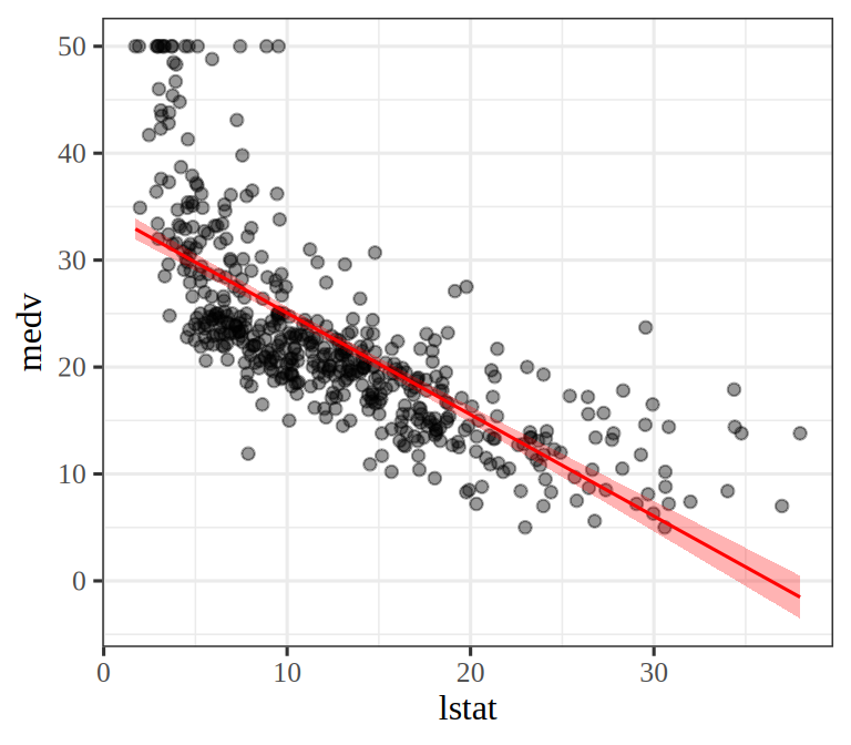
# The band is the 95% confidence interval for the mean medv at each lstatlstat_grid<-tibble(lstat =seq(min(boston$lstat), max(boston$lstat), length.out =100))boston_band<-bind_cols(lstat_grid,predict(tm_boston_simple, new_data =lstat_grid),predict(tm_boston_simple, new_data =lstat_grid, type ="conf_int"))ggplot()+geom_point(data =boston, aes(lstat, medv), alpha =0.4)+geom_ribbon(data =boston_band,aes(lstat, ymin =.pred_lower, ymax =.pred_upper), fill ="red", alpha =0.3)+geom_line(data =boston_band, aes(lstat, .pred), colour ="red")
Show code
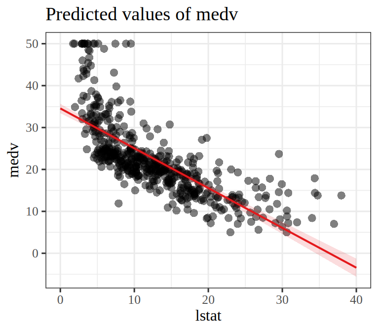
sjPlot::plot_model(lm_boston_simple, type ="pred", terms ="lstat", show.data =TRUE)
Figure 1: Typical home value against lstat for the Boston data, with a straight line inside a shaded band.
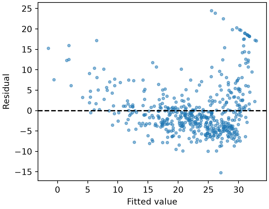
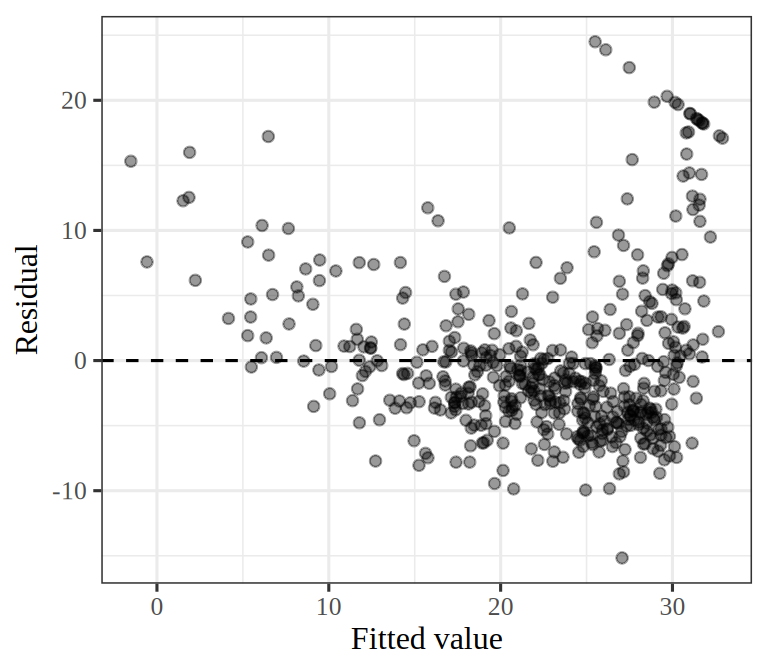
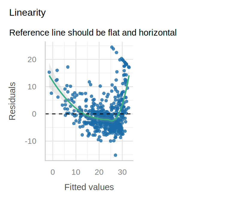
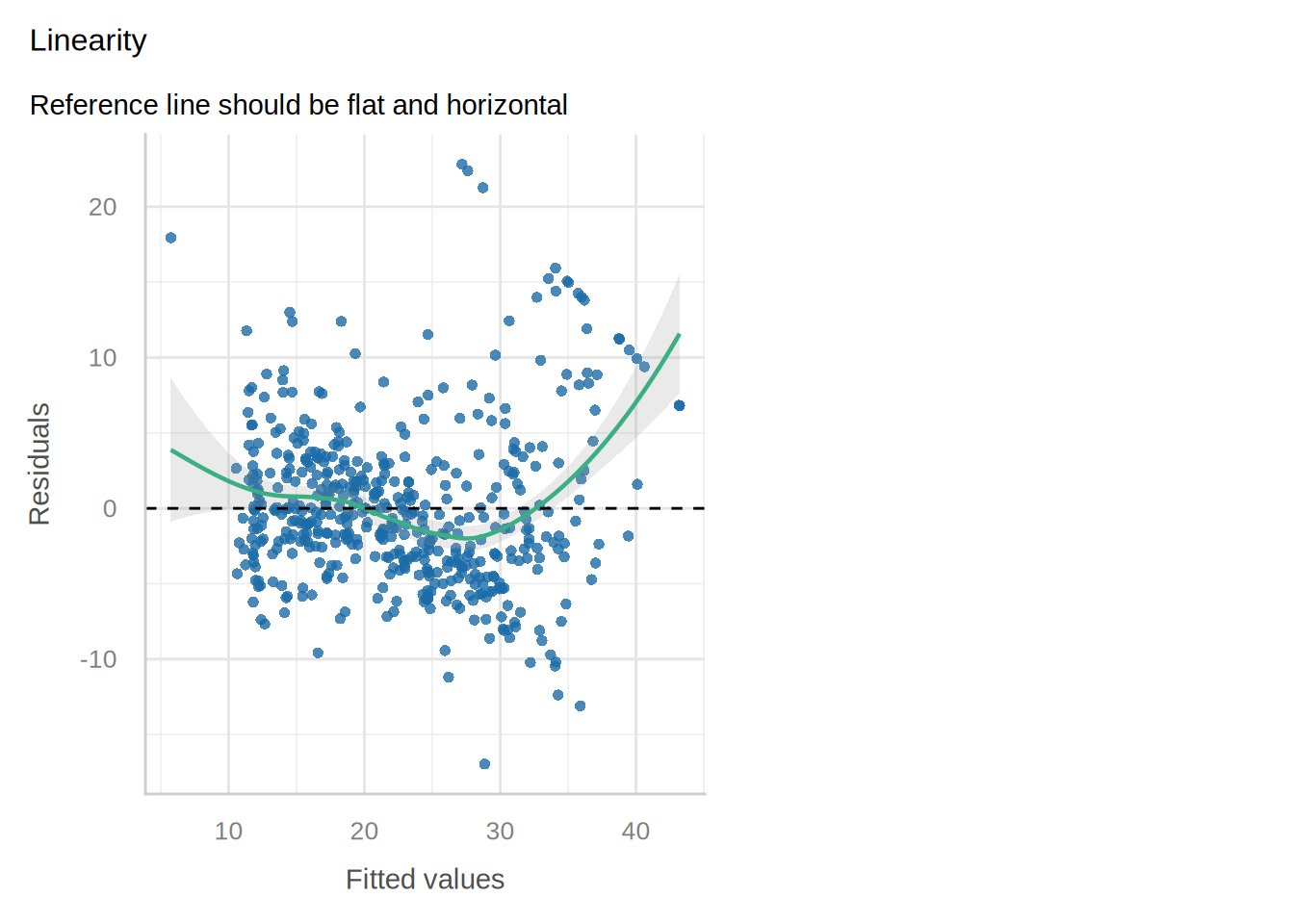
Solution 8. The points curve: they lie above the line at both ends and below it in the middle. The residual plot shows the same pattern as a U shape, the sign of non-linearity in a residual plot. Exercise 16 adds a squared term for it.
4 Multiple linear regression
ExrExercise 9 (Lab: many features on the Boston data)
Exercise 9 (Lab: many features on the Boston data) Fit medv on lstat and age, the percentage of owner-occupied homes built before 1940. How does the lstatcoefficient compare with that of Exercise 1?
library(tidymodels)# Each coefficient with its standard error and 95% confidence intervaltm_boston_lstat_age<-lm_spec|>fit(medv~lstat+age, data =boston)tidy(tm_boston_lstat_age, conf.int =TRUE)
# The table includes each coefficient's standard error# and 95% confidence intervallm_boston_lstat_age<-lm(medv~lstat+age, data =boston)parameters::parameters(lm_boston_lstat_age)|>parameters::print_md(digits =3)
Parameter
Coefficient
SE
95% CI
t(503)
p
(Intercept)
33.223
0.731
(31.787, 34.659)
45.458
< .001
lstat
-1.032
0.048
(-1.127, -0.937)
-21.416
< .001
age
0.035
0.012
(0.011, 0.059)
2.826
0.005
The lstat coefficient moves from -0.950 (95% confidence interval -1.026 to -0.874) to -1.032 (-1.127 to -0.937). It is now the change in medv per point of lstat among neighborhoods with the same age.
ExrExercise 10 (Lab: many features on the Boston data (part 2))
Exercise 10 (Lab: many features on the Boston data (part 2)) Use the setup of Exercise 9.
Solution 11. indus and age have \(p\)-values above \(0.05\). With the other features in the model, the data give no clear sign that either one adds anything.
ExrExercise 12 (Lab: many features on the Boston data (part 4))
Exercise 12 (Lab: many features on the Boston data (part 4)) Use the setup of Exercise 9.
from statsmodels.stats.outliers_influence import variance_inflation_factor as VIFvif = pd.DataFrame({"vif": [VIF(X_all, i) for i inrange(1, X_all.shape[1])]}, index=X_all.columns[1:])# A VIF has no formula for its interval, so bootstrap_vif_ci# (in the interval helpers) resamples the neighborhoodsvif[["lower", "upper"]] = bootstrap_vif_ci(Boston.drop(columns="medv")).Tprint(vif)
# A VIF has no formula for its interval, so boot_vif_ci# (in the interval helpers) resamples the neighborhoods# VIF_j = 1 / (1 - R^2) from regressing feature j on the other featurespredictors<-setdiff(names(boston), "medv")vif_interval<-boot_vif_ci(boston[predictors])tibble( feature =predictors, vif =map_dbl(predictors, \(feature){r_squared<-lm_spec|>fit(reformulate(setdiff(predictors, feature), feature), data =boston)|>glance()|>pull(r.squared)1/(1-r_squared)}), lower =vif_interval[1, ], upper =vif_interval[2, ])
# A VIF has no formula for its interval, so boot_vif_ci# (in the interval helpers) resamples the neighborhoods# VIF_j = 1 / (1 - R^2) from regressing feature j on the other featurespredictors<-setdiff(names(boston), "medv")vif_boston<-sapply(predictors, function(feature){others<-reformulate(setdiff(predictors, feature), feature)1/(1-summary(lm(others, data =boston))$r.squared)})vif_boston
# The same resampling gives an interval for the correlation of two features.# boot_cor_ci() is one of the interval helperscor(boston$tax, boston$rad)
[1] 0.9102282
boot_cor_ci(boston$tax, boston$rad)
[1] 0.8804014 0.9349518
The largest variance inflation factor is 9.00 (95% bootstrap interval 7.22 to 12.24), for tax, the property tax rate. Its coefficient has about 9 times the variance it would have if that feature were uncorrelated with the others. The next largest is 7.45 (6.18 to 9.91), for rad, the access to radial highways. The two are strongly correlated with each other (correlation 0.91, 95% bootstrap interval 0.88 to 0.93). Each bootstrap interval is the 2.5th to 97.5th percentile over 20,000 resamples of the \(506\) neighborhoods, with the statistic recomputed on each resample. Confidence intervals for the coefficients in the tables above are \(t\) intervals, the estimate plus or minus a \(t\) quantile times its standard error.
5 Interaction terms
ExrExercise 14 (Lab: an interaction on the Boston data)
Exercise 14 (Lab: an interaction on the Boston data) Fit medv on lstat, age and their product \(\text{lstat} \times \text{age}\), the interaction of the two features. Report the coefficients with their \(p\)-values.
library(tidymodels)interaction_recipe<-recipe(medv~lstat+age, data =boston)|>step_interact(~lstat:age)tm_boston_interaction<-workflow()|>add_recipe(interaction_recipe)|>add_model(lm_spec)|>fit(boston)# Each coefficient with its standard error and 95% confidence intervaltidy(tm_boston_interaction, conf.int =TRUE)
lm_boston_interaction<-lm(medv~lstat*age, data =boston)# The table includes each coefficient's standard error# and 95% confidence intervalparameters::parameters(lm_boston_interaction)|>parameters::print_md(digits =3)
Parameter
Coefficient
SE
95% CI
t(502)
p
(Intercept)
36.089
1.470
(33.201, 38.976)
24.553
< .001
lstat
-1.392
0.167
(-1.721, -1.063)
-8.313
< .001
age
-7.209e-04
0.020
(-0.040, 0.038)
-0.036
0.971
lstat × age
0.004
0.002
(5.177e-04, 0.008)
2.244
0.025
The interaction coefficient is 0.0042 (95% confidence interval 0.0005 to 0.0078), with \(p\)-value 0.025.
ExrExercise 15 (Lab: an interaction on the Boston data (part 2))
Exercise 15 (Lab: an interaction on the Boston data (part 2)) Use the setup of Exercise 14.
Is there evidence that the slope on lstat depends on age?
# The slope on lstat, beta_1 + beta_3 age,# is a linear combination of the coefficients,# so its 95% interval comes from lincomb_ci(),# one of the interval helpers,# with the weights (0, 1, 0, age)slope_age_20<-lincomb_ci(lm_boston_interaction, c(0, 1, 0, 20))slope_age_90<-lincomb_ci(lm_boston_interaction, c(0, 1, 0, 90))
That is modest evidence that the slope on lstat depends on age. The fitted slope on lstat is \(\hcoef{1} + \hcoef{3} \cdot \text{age}\). It is about -1.31 (95% confidence interval -1.57 to -1.05) in a neighborhood where \(20\%\) of homes were built before 1940, and about -1.02 (-1.11 to -0.92) where \(90\%\) were. Each interval is a \(t\) interval, the estimate plus or minus a \(t\) quantile times its standard error, and the standard error of the slope comes from the coefficients’ estimatedcovariance matrix. The main effect of age has \(p\)-value 0.97, but the hierarchy principle keeps it in the model alongside its interaction.
Exercise 16 (Lab: a curve in lstat) Add \(\text{lstat}^2\) to the model of Exercise 9, so the features are lstat, \(\text{lstat}^2\) and age. Report the coefficients with their \(p\)-values.
TipHint
Wrap the square in I(...) inside the formula so that ** is read as a power. In R, write ^ instead of **.
library(tidymodels)quadratic_recipe<-recipe(medv~lstat+age, data =boston)|>step_mutate(lstat2 =lstat^2)tm_boston_quadratic<-workflow()|>add_recipe(quadratic_recipe)|>add_model(lm_spec)|>fit(boston)# Each coefficient with its standard error and 95% confidence intervaltidy(tm_boston_quadratic, conf.int =TRUE)
lm_boston_quadratic<-lm(medv~lstat+I(lstat^2)+age, data =boston)# The table includes each coefficient's standard error# and 95% confidence intervalparameters::parameters(lm_boston_quadratic)|>parameters::print_md(digits =3)
Parameter
Coefficient
SE
95% CI
t(502)
p
(Intercept)
41.289
0.873
(39.573, 43.004)
47.284
< .001
lstat
-2.688
0.131
(-2.946, -2.431)
-20.502
< .001
lstat^2
0.049
0.004
(0.042, 0.057)
13.315
< .001
age
0.070
0.011
(0.049, 0.092)
6.471
< .001
The coefficient of \(\text{lstat}^2\) is 0.0495 (95% confidence interval 0.0422 to 0.0568, the estimate plus or minus a \(t\) quantile times its standard error), with \(p\)-value \(7.5\times10^{-35}\). The positive sign means the fitted curve flattens as lstat grows, as the scatter plot of Solution 6 suggested.
from statsmodels.stats.anova import anova_lmprint(anova_lm(boston_lstat_age, boston_quadratic))
   df_resid           ssr  df_diff      ss_diff           F        Pr(>F)
0     503.0  19168.128609      0.0          NaN         NaN           NaN
1     502.0  14165.613251      1.0  5002.515357  177.278785  7.468491e-35
# anova() compares models only when their responses have the same name,# so fit the smaller model through a workflow too.tm_boston_lstat_age_wf<-workflow()|>add_recipe(recipe(medv~lstat+age, data =boston))|>add_model(lm_spec)|>fit(boston)anova(extract_fit_engine(tm_boston_lstat_age_wf),extract_fit_engine(tm_boston_quadratic))|>tidy()
Solution 18. The squared term clearly improves the fit. Since \(q = 1\), the \(F\)-statistic is the square of the \(t\)-statistic of \(\text{lstat}^2\) (13.31\(^2\)\(=\) 177.3).
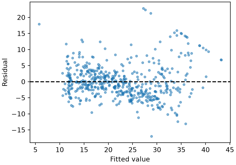
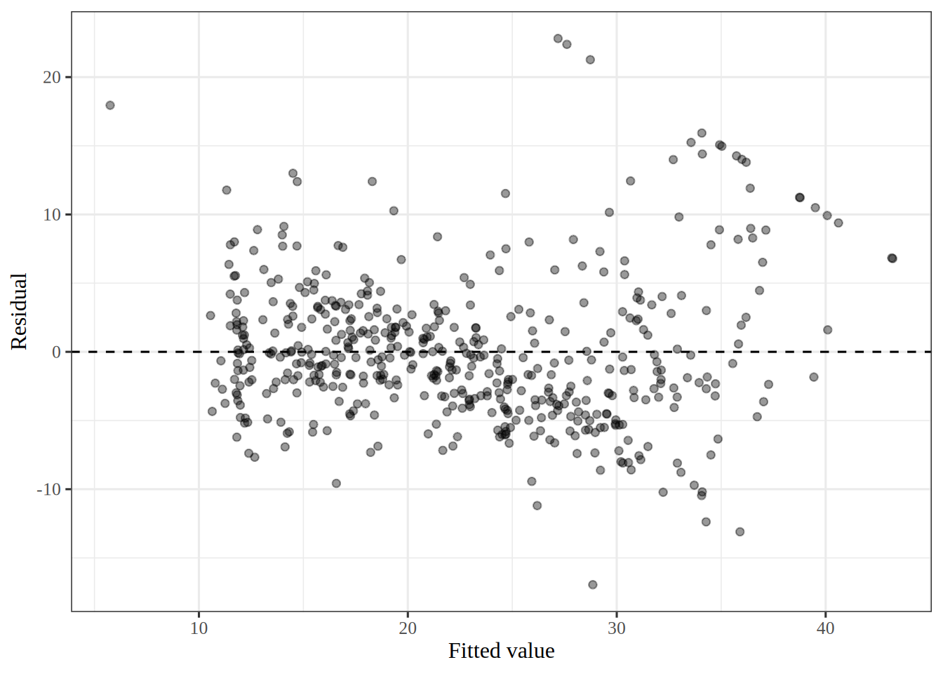
Solution 20. The U shape of the first residual plot is gone: the residuals now scatter around \(0\) across the fitted values, though their spread grows at the highest fitted values.
7 Qualitative predictors
ExrExercise 21 (Lab: a category with three levels)
Exercise 21 (Lab: a category with three levels) Download the Carseats data from data/carseats.csv and save it as data/carseats.csv next to your code. It is simulated data on sales of child car seats at \(400\) stores, from the book [1]. Sales is unit sales in thousands. ShelveLoc is the quality of the shelf space for the car seats at each store: Bad, Medium or Good.
Fit Sales on all the other columns, plus the interactions \(\text{Income} \times \text{Advertising}\) and \(\text{Price} \times \text{Age}\).
TipHint
In a formula, Income:Advertising adds only the product, and a column of text is treated as a category automatically.
import pandas as pdimport statsmodels.api as sm# ISLP's load_data("Carseats") reads this same file.Carseats = pd.read_csv("data/carseats.csv")sales = Carseats["Sales"]X_carseats = pd.get_dummies(Carseats.drop(columns="Sales"), drop_first=True, dtype=float)X_carseats["Income:Advertising"] = Carseats["Income"] * Carseats["Advertising"]X_carseats["Price:Age"] = Carseats["Price"] * Carseats["Age"]X_carseats = sm.add_constant(X_carseats)carseats_fit = sm.OLS(sales, X_carseats).fit()# The table includes each coefficient's standard error# and 95% confidence intervalprint(carseats_fit.summary2().tables[1])
library(tidymodels)carseats<-read.csv("data/carseats.csv")carseats_recipe<-recipe(Sales~., data =carseats)|>step_dummy(all_nominal_predictors())|>step_interact(~Income:Advertising+Price:Age)tm_carseats<-workflow()|>add_recipe(carseats_recipe)|>add_model(lm_spec)|>fit(carseats)# Each coefficient with its standard error and 95% confidence intervaltidy(tm_carseats, conf.int =TRUE)
carseats<-read.csv("data/carseats.csv", stringsAsFactors =TRUE)lm_carseats<-lm(Sales~.+Income:Advertising+Price:Age, data =carseats)# The table includes each coefficient's standard error# and 95% confidence intervalparameters::parameters(lm_carseats)|>parameters::print_md(digits =3)
Parameter
Coefficient
SE
95% CI
t(386)
p
(Intercept)
6.576
1.009
(4.592, 8.559)
6.519
< .001
CompPrice
0.093
0.004
(0.085, 0.101)
22.567
< .001
Income
0.011
0.003
(0.006, 0.016)
4.183
< .001
Advertising
0.070
0.023
(0.026, 0.115)
3.107
0.002
Population
1.592e-04
3.679e-04
(-5.640e-04, 8.825e-04)
0.433
0.665
Price
-0.101
0.007
(-0.115, -0.086)
-13.549
< .001
ShelveLoc (Good)
4.849
0.153
(4.548, 5.149)
31.724
< .001
ShelveLoc (Medium)
1.953
0.126
(1.706, 2.201)
15.531
< .001
Age
-0.058
0.016
(-0.089, -0.027)
-3.633
< .001
Education
-0.021
0.020
(-0.059, 0.018)
-1.063
0.288
Urban (Yes)
0.140
0.112
(-0.081, 0.361)
1.247
0.213
US (Yes)
-0.158
0.149
(-0.450, 0.135)
-1.058
0.291
Income × Advertising
7.510e-04
2.784e-04
(2.037e-04, 0.001)
2.698
0.007
Price × Age
1.068e-04
1.333e-04
(-1.554e-04, 3.689e-04)
0.801
0.424
The fit has 14 coefficients: an intercept, the 10 other columns with ShelveLoc expanded into two indicators, and the two products.
ExrExercise 22 (Lab: a category with three levels (part 2))
Exercise 22 (Lab: a category with three levels (part 2)) Use the setup of Exercise 21.
Which indicator columns does the software build for ShelveLoc?
TipHint
The category terms of a formula name one indicator column for each level except the baseline; read the names in the summary.
Solution 23. Bad has no column of its own: it is the baseline, where both indicators are \(0\). Each tool drops the first level in alphabetical order, and Bad comes first.
ExrExercise 24 (Lab: a category with three levels (part 4))
Exercise 24 (Lab: a category with three levels (part 4)) Use the setup of Exercise 21.
Interpret the coefficients of the two ShelveLoc indicators.
TipHint
Each coefficient of an indicator is a difference from the baseline, with the other features held fixed.
Solution 24. The Goodcoefficient is 4.85 (95% confidence interval 4.55 to 5.15). A store with a good shelf location is predicted to sell about 4,850 more car seats (95% confidence interval 4,550 to 5,150 seats) than a store with a bad one, with the other features held fixed. The Medium coefficient is 1.95 (1.71 to 2.20), so a medium location sits between the two, about 1,950 seats above a bad one (1,710 to 2,200 seats). Each interval is a \(t\) interval, the estimate plus or minus a \(t\) quantile times its standard error.
References
[1]
G. James, D. Witten, T. Hastie, R. Tibshirani, and J. Taylor, An introduction to statistical learning: With applications in Python. Springer, 2023. doi: 10.1007/978-3-031-38747-0.
[2]
D. Harrison and D. L. Rubinfeld, “Hedonic housing prices and the demand for clean air,”Journal of Environmental Economics and Management, vol. 5, no. 1, pp. 81–102, 1978, doi: 10.1016/0095-0696(78)90006-2.