Linear Regression on the Auto Data

Published

Last modified: 2026-11-19

Show code
# The Python chunks import numpy, pandas, matplotlib, scipy and statsmodels;
# reticulate provisions them.
library(reticulate) # nolint: undesirable_function_linter
py_packages <- c("numpy", "pandas", "matplotlib", "scipy", "statsmodels")
py_require(py_packages)
# A positive number in scientific notation, for display math: 2.4\times10^{2}.
sci <- function(v) { # nolint: function_location_linter
  e <- v |> log10() |> floor()
  m <- signif(v / 10^e, 2)
  carry <- m >= 10
  if (carry) {
    m <- m / 10
    e <- e + 1
  }
  sprintf("%.1f\\times10^{%d}", m, e)
}

This material was part of the linear regression page. The lab exercises are adapted from the lab that accompanies [1, Ch. 3]. The concepts that the lab applies are on the page Interactions, Inference and Diagnostics. The lab on the Boston and Carseats data follows the book more closely, and has downloadable stubs.

1 Lab: linear regression on the Auto data

The lab exercises in this section and the next are adapted from the lab that accompanies [1, Ch. 3], whose Python code is published as ISLP_labs. The book’s lab uses the Boston and Carseats data and the statsmodels package; here the same steps use the Auto data. Each solution gives the code in Python with statsmodels, as the book’s lab does; in Python with the np.linalg.lstsq of this chapter; in R with tidymodels; and in base R. The tidymodels code follows ISLR-tidymodels-labs, the tidymodels version of the book’s labs.

Every lab and example below reports 95% confidence intervals. These helpers are defined once, here, so no page depends on another page’s code. Each takes all its inputs as arguments.

Show code
import numpy as np


def bootstrap_corr_ci(a, b, B=20000, seed=571):
    """95% percentile interval for the correlation of a and b.

    Resamples the cases with replacement B times,
    which mimics drawing new cases from the same population,
    and recomputes the correlation each time.
    """
    rng = np.random.default_rng(seed)
    a, b = np.asarray(a, float), np.asarray(b, float)
    corr = np.empty(B)
    for i in range(B):
        rows = rng.integers(0, len(a), len(a))
        corr[i] = np.corrcoef(a[rows], b[rows])[0, 1]
    return np.quantile(corr, [0.025, 0.975])


def bootstrap_vif_ci(features, B=20000, seed=571):
    """95% percentile interval for each feature's VIF.

    The VIF of feature j is the jth diagonal entry
    of the inverse of the features' correlation matrix,
    which gives the same value as 1 / (1 - R^2) without a regression per feature.
    """
    rng = np.random.default_rng(seed)
    F = np.asarray(features, float)
    vifs = np.empty((B, F.shape[1]))
    for b in range(B):
        rows = rng.integers(0, len(F), len(F))
        vifs[b] = np.diag(np.linalg.inv(np.corrcoef(F[rows], rowvar=False)))
    return np.quantile(vifs, [0.025, 0.975], axis=0)
Show code
# Formats an interval's endpoints for the prose
ci_text <- function(bounds, digits) {
  sprintf("%.*f to %.*f", digits, bounds[[1]], digits, bounds[[2]])
}

# 95% percentile interval for R^2 from resampled cars.
# Resampling rows with replacement mimics
# drawing a new set of cars from the same population.
# The refits use lm.fit directly, because 2,000 workflow fits would be slow.
boot_r2_ci <- function(formula, data, n_boot = 2000) {
  set.seed(571)
  design <- model.matrix(formula, data)
  y <- model.response(model.frame(formula, data))
  r2 <- vapply(seq_len(n_boot), \(b) {
    rows <- sample(nrow(design), replace = TRUE)
    sse <- sum(lm.fit(design[rows, ], y[rows])$residuals^2)
    1 - sse / sum((y[rows] - mean(y[rows]))^2)
  }, numeric(1))
  unname(quantile(r2, c(0.025, 0.975)))
}

# 95% percentile interval for the correlation of a and b
boot_cor_ci <- function(a, b, n_boot = 20000) {
  set.seed(571)
  corr <- vapply(seq_len(n_boot), \(i) {
    rows <- sample(length(a), replace = TRUE)
    cor(a[rows], b[rows])
  }, numeric(1))
  unname(quantile(corr, c(0.025, 0.975)))
}

# 95% percentile interval for each feature's VIF.
# The VIF of feature j is the jth diagonal entry
# of the inverse of the features' correlation matrix,
# which gives the same value as 1 / (1 - R^2) without a regression per feature.
boot_vif_ci <- function(features, n_boot = 20000) {
  set.seed(571)
  vifs <- vapply(seq_len(n_boot), \(b) {
    resample <- features[sample(nrow(features), replace = TRUE), ]
    diag(solve(cor(resample)))
  }, numeric(ncol(features)))
  apply(vifs, 1, quantile, probs = c(0.025, 0.975))
}

# The 95% interval for a linear combination w'beta
# of a fitted model's coefficients:
# the estimate plus or minus a t quantile times its standard error,
# from the coefficients' covariance matrix
lincomb_ci <- function(model, w) {
  estimate <- sum(w * coef(model))
  half <- qt(0.975, df.residual(model)) * sqrt(drop(t(w) %*% vcov(model) %*% w))
  c(estimate = estimate, lower = estimate - half, upper = estimate + half)
}
ExrExercise 1 (Lab: fit a line to the Auto data)

Exercise 1 (Lab: fit a line to the Auto data) This exercise is the first of six short lab exercises on the Auto data. Work in pairs, at a computer. Use Python or R; each solution shows both.

Download the Auto data from data/auto.csv, the file used in this chapter. Save it as data/auto.csv next to your code, because the solutions read it from that path. It has \(392\) cars, and comes from the book [1]; the Python package ISLP and the R package ISLR2 also provide it.

Predict a car’s fuel economy mpg from its horsepower.

Load the data and look at its first rows.

Solution 1.

import numpy as np
import pandas as pd
import statsmodels.api as sm

# ISLP's load_data("Auto") reads this same file.
Auto = pd.read_csv("data/auto.csv")
print(Auto.head())
    mpg  cylinders  displacement  ...  year  origin                       name
0  18.0          8         307.0  ...    70       1  chevrolet chevelle malibu
1  15.0          8         350.0  ...    70       1          buick skylark 320
2  18.0          8         318.0  ...    70       1         plymouth satellite
3  16.0          8         304.0  ...    70       1              amc rebel sst
4  17.0          8         302.0  ...    70       1                ford torino

[5 rows x 9 columns]
import numpy as np
import pandas as pd
from scipy import stats

# ISLP's load_data("Auto") reads this same file.
Auto = pd.read_csv("data/auto.csv")
print(Auto.head())
    mpg  cylinders  displacement  ...  year  origin                       name
0  18.0          8         307.0  ...    70       1  chevrolet chevelle malibu
1  15.0          8         350.0  ...    70       1          buick skylark 320
2  18.0          8         318.0  ...    70       1         plymouth satellite
3  16.0          8         304.0  ...    70       1              amc rebel sst
4  17.0          8         302.0  ...    70       1                ford torino

[5 rows x 9 columns]

y = Auto["mpg"].to_numpy()
horsepower = Auto["horsepower"].to_numpy(float)
weight = Auto["weight"].to_numpy(float)
n = len(y)
library(tidymodels)

auto <- read.csv("data/auto.csv")
lm_spec <- linear_reg() |> set_engine("lm")
auto <- read.csv("data/auto.csv")
head(auto)

1. The file has 392 rows, one per car.

ExrExercise 2 (Lab: fit a line to the Auto data (part 2))

Exercise 2 (Lab: fit a line to the Auto data (part 2)) Use the setup of Exercise 1.

Build the design matrix \(\design\) with a column of ones and a column of horsepower. Compute \(\hvcoef\) with np.linalg.lstsq in Python, or lm() in R.

Solution 2.

mpg = Auto["mpg"]
X_auto_simple = pd.DataFrame({"intercept": np.ones(Auto.shape[0]),
                              "horsepower": Auto["horsepower"]})
auto_simple = sm.OLS(mpg, X_auto_simple).fit()

# Each coefficient with its 95% confidence interval
print(pd.concat([auto_simple.params, auto_simple.conf_int()], axis=1)
      .set_axis(["coef", "lower", "upper"], axis=1))
                 coef      lower      upper
intercept   39.935861  38.525212  41.346510
horsepower  -0.157845  -0.170517  -0.145172
def fit(columns):
    Phi = np.column_stack([np.ones(n)] + columns)
    beta_hat = np.linalg.lstsq(Phi, y, rcond=None)[0]
    return beta_hat, Phi

def mean_squared_error(beta_hat, Phi):
    return np.mean((Phi @ beta_hat - y) ** 2)

def rmse(beta_hat, Phi):
    return np.sqrt(mean_squared_error(beta_hat, Phi))

def r_squared(beta_hat, Phi):
    sst = np.sum((y - y.mean()) ** 2)
    return 1 - mean_squared_error(beta_hat, Phi) * n / sst

def ols_summary(beta_hat, Phi, y_obs=y):
    """Residual degrees of freedom, the estimated noise variance, and (Phi'Phi)^{-1}."""
    df = len(y_obs) - Phi.shape[1]
    sigma2 = np.sum((y_obs - Phi @ beta_hat) ** 2) / df
    # The pseudoinverse gives (Phi'Phi)^{-1} without forming Phi'Phi,
    # which is badly conditioned for high-degree polynomials
    pinv = np.linalg.pinv(Phi)
    return df, sigma2, pinv @ pinv.T

def coef_ci(beta_hat, Phi):
    """95% interval for each coefficient: the estimate plus or minus a t quantile times its standard error."""
    df, sigma2, PtP_inv = ols_summary(beta_hat, Phi)
    half = stats.t.ppf(0.975, df) * np.sqrt(sigma2 * np.diag(PtP_inv))
    return np.column_stack([beta_hat - half, beta_hat + half])

def contrast_ci(beta_hat, Phi, c):
    """95% interval for the linear combination c'beta of the coefficients."""
    df, sigma2, PtP_inv = ols_summary(beta_hat, Phi)
    half = stats.t.ppf(0.975, df) * np.sqrt(sigma2 * c @ PtP_inv @ c)
    return c @ beta_hat - half, c @ beta_hat + half

def mean_ci(beta_hat, Phi, Phi_new, prediction=False, y_obs=y):
    """95% interval at the rows of Phi_new: for the mean response, or with prediction=True for one new response."""
    df, sigma2, PtP_inv = ols_summary(beta_hat, Phi, y_obs)
    # The variance of the fitted value, plus the noise of one new response for a prediction interval
    variance = sigma2 * (np.sum((Phi_new @ PtP_inv) * Phi_new, axis=1) + prediction)
    half = stats.t.ppf(0.975, df) * np.sqrt(variance)
    fitted_new = Phi_new @ beta_hat
    return fitted_new - half, fitted_new + half

def bootstrap_r2_ci(Phi, B=2000, seed=571):
    """95% percentile interval for R^2 from B resamples of the cars, refitted each time."""
    rng = np.random.default_rng(seed)
    r2 = np.empty(B)
    for b in range(B):
        rows = rng.integers(0, n, n)
        beta_b = np.linalg.lstsq(Phi[rows], y[rows], rcond=None)[0]
        sse = np.sum((y[rows] - Phi[rows] @ beta_b) ** 2)
        r2[b] = 1 - sse / np.sum((y[rows] - y[rows].mean()) ** 2)
    return np.quantile(r2, [0.025, 0.975])
beta_simple, Phi_simple = fit([horsepower])
print(np.column_stack([beta_simple, coef_ci(beta_simple, Phi_simple)]))
[[39.93586102 38.52521179 41.34651025]
 [-0.15784473 -0.17051701 -0.14517246]]
# Each coefficient with its 95% confidence interval
tm_simple <- lm_spec |> fit(mpg ~ horsepower, data = auto)
tidy(tm_simple, conf.int = TRUE)
fit_simple <- lm(mpg ~ horsepower, data = auto)
# The table includes each coefficient's 95% confidence interval
parameters::parameters(fit_simple) |>
  parameters::print_md(digits = 4)
Parameter Coefficient SE 95% CI t(390) p
(Intercept) 39.9359 0.7175 (38.5252, 41.3465) 55.6598 < .001
horsepower -0.1578 0.0064 (-0.1705, -0.1452) -24.4891 < .001
Show code
coef_ci_simple <- py$coef_ci(py$beta_simple, py$Phi_simple)
rmse_simple <- py$rmse(py$beta_simple, py$Phi_simple)

2.

The fit uses \(n =\) 392 cars. The line is \(\widehat{\text{mpg}} =\) 39.9 \(-\) 0.158 \(\times\) horsepower. Each 95% confidence interval for a coefficient in the coefficient tables is the estimate plus or minus a \(t\) quantile times its standard error. The intercept’s interval is 38.5 to 41.3, and the slope’s is -0.171 to -0.145.

ExrExercise 3 (Lab: fit a line to the Auto data (part 3))

Exercise 3 (Lab: fit a line to the Auto data (part 3)) Use the setup of Exercise 1.

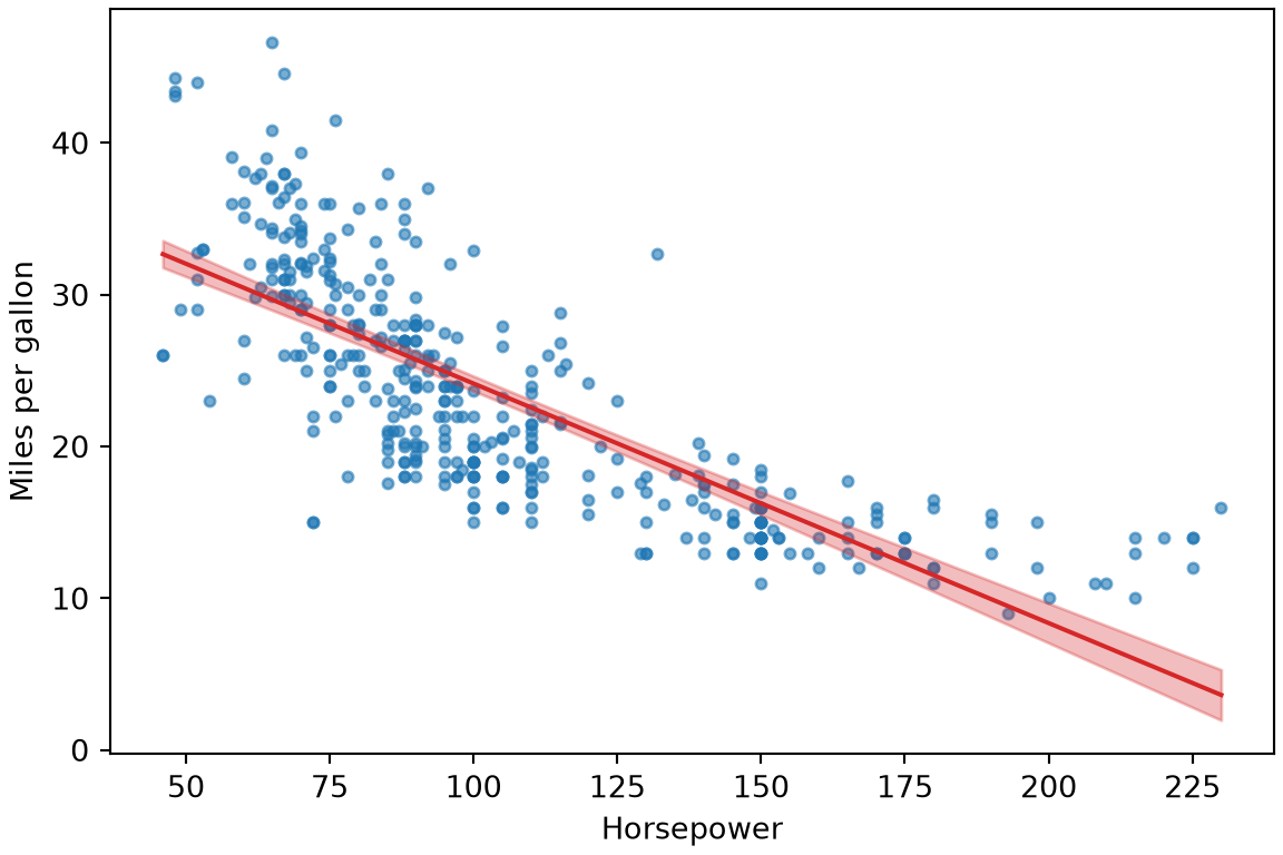
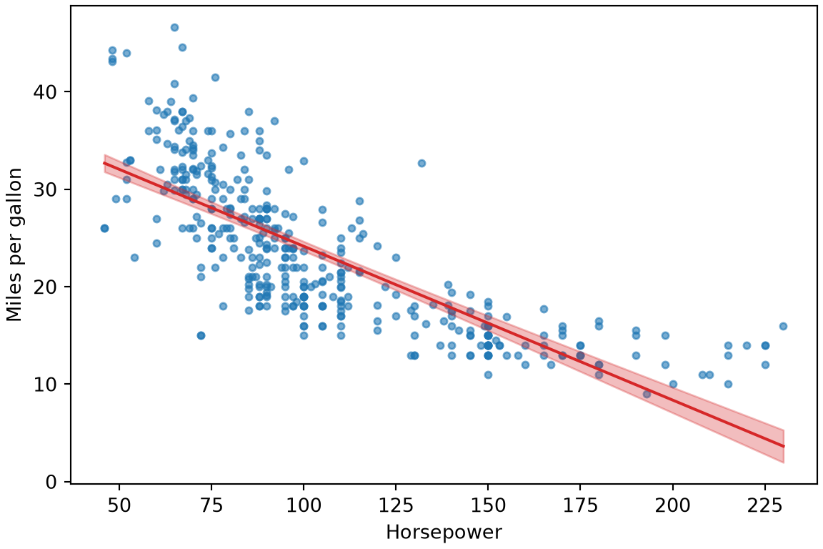
Draw a scatter plot of mpg against horsepower with the fitted line. Does a straight line describe the pattern well?

Solution 3.

Show code
import matplotlib.pyplot as plt
import numpy as np

hp_grid = np.linspace(Auto["horsepower"].min(), Auto["horsepower"].max(), 100)
# The band is the 95% confidence interval for the mean mpg at each horsepower
band = auto_simple.get_prediction(
    pd.DataFrame({"intercept": 1.0, "horsepower": hp_grid})).conf_int(alpha=0.05)
fig, ax = plt.subplots(figsize=(6, 4), layout="constrained")
ax.scatter(Auto["horsepower"], mpg, s=12, alpha=0.6);
ax.fill_between(hp_grid, band[:, 0], band[:, 1], color="C3", alpha=0.3);
ax.plot(hp_grid,
        auto_simple.params["intercept"] + auto_simple.params["horsepower"] * hp_grid,
        color="C3");
ax.set_xlabel("Horsepower");
ax.set_ylabel("Miles per gallon");
plt.show()
Show code
import matplotlib.pyplot as plt

grid = np.linspace(horsepower.min(), horsepower.max(), 100)
Phi_grid = np.column_stack([np.ones(100), grid])
band_lower, band_upper = mean_ci(beta_simple, Phi_simple, Phi_grid)
fig, ax = plt.subplots(figsize=(6, 4), layout="constrained")
ax.scatter(horsepower, y, s=12, alpha=0.6);
ax.fill_between(grid, band_lower, band_upper, color="C3", alpha=0.3);
ax.plot(grid, beta_simple[0] + beta_simple[1] * grid, color="C3");
ax.set_xlabel("Horsepower");
ax.set_ylabel("Miles per gallon");
plt.show()
Show code
library(tidymodels)

# The band is the 95% confidence interval for the mean mpg at each horsepower
hp_grid <- tibble(horsepower = seq(min(auto$horsepower), max(auto$horsepower),
                                   length.out = 100))
simple_band <- bind_cols(
  hp_grid,
  predict(tm_simple, new_data = hp_grid),
  predict(tm_simple, new_data = hp_grid, type = "conf_int")
)
ggplot() +
  geom_point(data = auto, aes(horsepower, mpg), alpha = 0.4) +
  geom_ribbon(data = simple_band,
              aes(horsepower, ymin = .pred_lower, ymax = .pred_upper),
              fill = "red", alpha = 0.3) +
  geom_line(data = simple_band, aes(horsepower, .pred), colour = "red") +
  labs(x = "Horsepower", y = "Miles per gallon")
Show code
sjPlot::plot_model(fit_simple, type = "pred", terms = "horsepower",
                   show.data = TRUE, title = "") +
  ggplot2::labs(x = "Horsepower", y = "Miles per gallon")
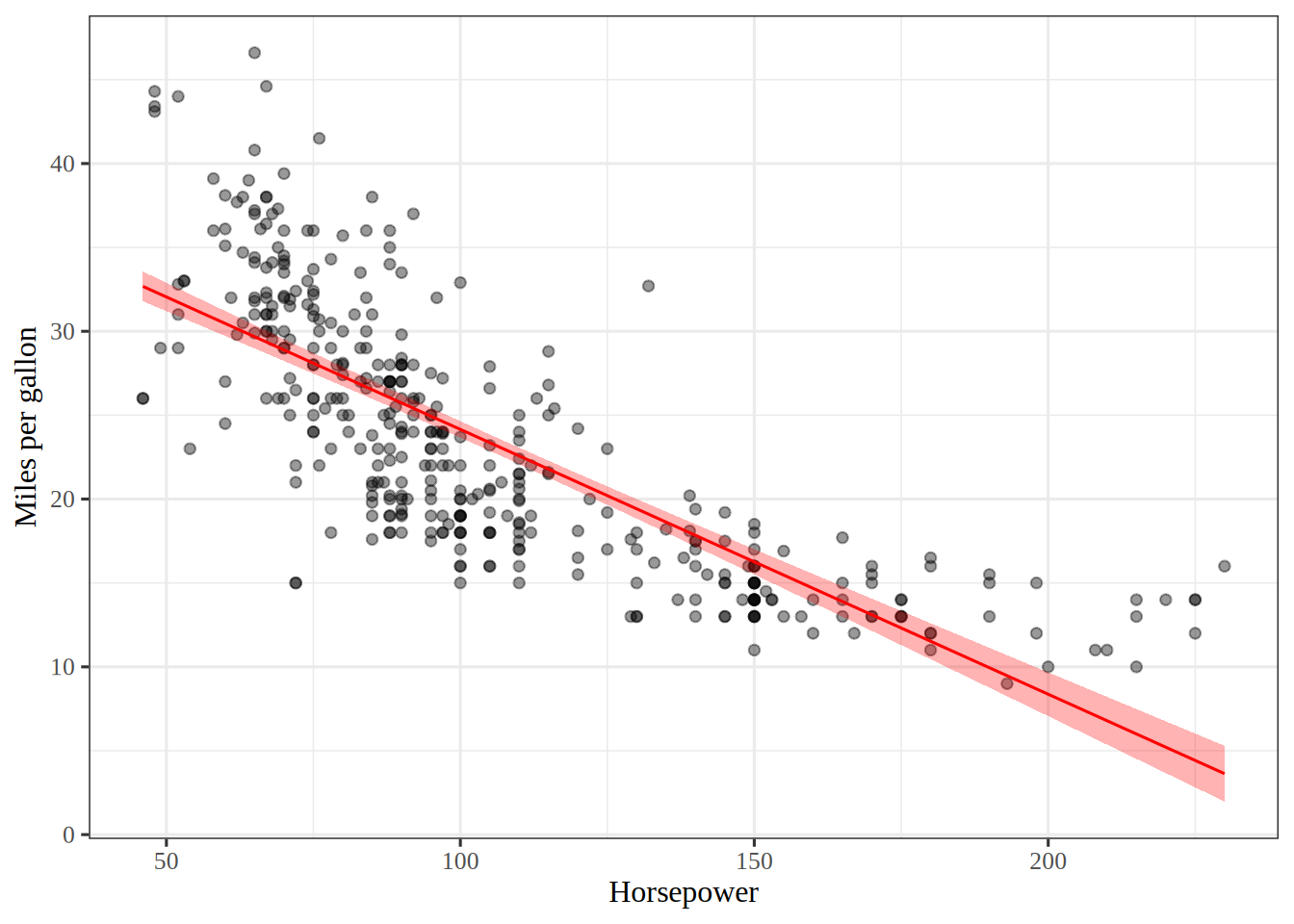
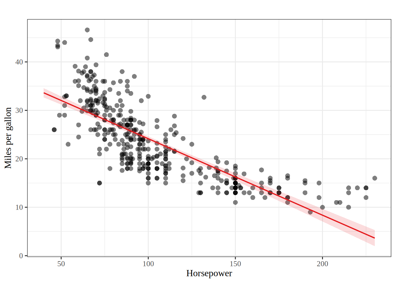
Figure 1: Miles per gallon against horsepower for the Auto data, with a straight line inside a shaded band.

3. The scatter plot shows a curve, not a line: the points bend, and the line misses them in the same direction at both ends. That is the pattern a later exercise fixes with a quadratic term. Figure 1 shows the line inside a shaded band. The shaded band in the figure is the 95% confidence interval for the mean mpg at every horsepower.

ExrExercise 4 (Lab: fit a line to the Auto data (part 4))

Exercise 4 (Lab: fit a line to the Auto data (part 4)) Use the setup of Exercise 1.

Compute the sMSE and \(R^2 = 1 - \text{SSE}/\text{SST}\), where SSE is the sum of squared residuals and SST is the sum of squared deviations of mpg from its sample mean.

Solution 4.

# Training root mean squared error, in miles per gallon
print(np.sqrt(auto_simple.ssr / auto_simple.nobs))
4.8932262300657134
print(auto_simple.rsquared)
0.6059482578894348
# R^2 has no formula for its interval, so refit on resampled cars.
# Resampling rows with replacement mimics drawing a new set of 392 cars from the same population.
def bootstrap_rsquared_ci(X, B=2000, seed=571):
    """95% percentile interval for R^2 from B resamples of the cars."""
    rng = np.random.default_rng(seed)
    X_arr, mpg_arr = np.asarray(X, float), mpg.to_numpy()
    rsquared = np.empty(B)
    for b in range(B):
        rows = rng.integers(0, len(mpg_arr), len(mpg_arr))
        rsquared[b] = sm.OLS(mpg_arr[rows], X_arr[rows]).fit().rsquared
    return np.quantile(rsquared, [0.025, 0.975])

print(bootstrap_rsquared_ci(X_auto_simple))
[0.55644218 0.65267338]
print(rmse(beta_simple, Phi_simple))
4.893226230065713
print(r_squared(beta_simple, Phi_simple))
0.6059482578894351
r2_ci_simple = bootstrap_r2_ci(Phi_simple)
print(r2_ci_simple)
[0.55644218 0.65267338]
# Training root mean squared error and R^2 of a fitted model
auto_metrics <- function(model, data = auto) {
  augment(model, new_data = data) |>
    summarise(rmse = sqrt(mean((mpg - .pred)^2)),
              r_squared = rsq_trad_vec(mpg, .pred))
}
auto_metrics(tm_simple)
# R^2 has no formula for its interval,
# so boot_r2_ci (in the interval helpers) refits on resampled cars.
boot_r2_ci(mpg ~ horsepower, auto)
[1] 0.5598592 0.6525384
rmse <- function(model) sqrt(mean(residuals(model)^2))
r_squared <- function(model) summary(model)$r.squared
c(rmse = rmse(fit_simple), r_squared = r_squared(fit_simple))
     rmse r_squared 
4.8932262 0.6059483 
# R^2 has no formula for its interval,
# so boot_r2_ci (in the interval helpers) refits on resampled cars.
boot_r2_ci(mpg ~ horsepower, auto)
[1] 0.5598592 0.6525384

4. The exercise asks for the sample mean squared error (sMSE); we report its square root, the sample root mean squared error (sRMSE), which is in miles per gallon (why we report sRMSE). The training sRMSE is 4.9 miles per gallon. It has no interval, because the same cars chose the coefficients and measure the error, so it understates the error on new cars, and an interval around it would describe the wrong quantity. The coefficient of determination is \(R^2 =\) 0.61, with a 95% bootstrap interval of 0.56 to 0.65: the 2.5th and 97.5th percentiles of \(R^2\) over 2,000 resamples of the cars drawn with replacement, each resample refitted. The Python and R tabs draw different random resamples, so their bootstrap endpoints agree only up to simulation error.

ExrExercise 5 (Lab: fit a line to the Auto data (part 5))

Exercise 5 (Lab: fit a line to the Auto data (part 5)) Use the setup of Exercise 1.

Predict mpg for a car with \(98\) horsepower. Say in words what the slope means.

Solution 5.

# The prediction for a 98-horsepower car, with the confidence interval for the mean
# (mean_ci_*) and the prediction interval for one car (obs_ci_*)
new_car = pd.DataFrame({"intercept": [1.0], "horsepower": [98]})
print(auto_simple.get_prediction(new_car).summary_frame(alpha=0.05).to_string())
        mean   mean_se  mean_ci_lower  mean_ci_upper  obs_ci_lower  obs_ci_upper
0  24.467077  0.251262      23.973079      24.961075     14.809396     34.124758
# The prediction for a 98-horsepower car, with the interval for the mean and for one car
Phi_98 = np.array([[1.0, 98.0]])
print(beta_simple @ [1, 98])
24.467077152512417
mean_ci_98 = np.array(mean_ci(beta_simple, Phi_simple, Phi_98)).ravel()
pred_ci_98 = np.array(mean_ci(beta_simple, Phi_simple, Phi_98, prediction=True)).ravel()
print(mean_ci_98, pred_ci_98)
[23.97307896 24.96107534] [14.80939607 34.12475823]
# The prediction for a 98-horsepower car,
# with the interval for the mean and for one car
new_car <- tibble(horsepower = 98)
predict(tm_simple, new_data = new_car)
predict(tm_simple, new_data = new_car, type = "conf_int")
predict(tm_simple, new_data = new_car, type = "pred_int")
# The prediction for a 98-horsepower car,
# with the interval for the mean and for one car
new_car <- tibble::tibble(horsepower = 98)
predict(fit_simple, new_car, interval = "confidence")
       fit      lwr      upr
1 24.46708 23.97308 24.96108
predict(fit_simple, new_car, interval = "prediction")
       fit     lwr      upr
1 24.46708 14.8094 34.12476

5. A \(98\)-horsepower car is predicted to get 24.5 miles per gallon. The 95% confidence interval for the mean response of such cars is 24.0 to 25.0, and the 95% prediction interval for one such car is 14.8 to 34.1. The prediction interval is wider because it includes the noise of a single car around the line.

The slope says that, across these cars, each extra horsepower goes with 0.16 fewer miles per gallon on average (95% confidence interval 0.15 to 0.17 fewer). It describes a pattern in the data, and does not say what would happen to one car if its engine were changed.

ExrExercise 6 (Lab: add a second feature)

Exercise 6 (Lab: add a second feature) Add weight to the model of Exercise 1.

Fit mpg on horsepower and weight. Report the coefficients, the sMSE and \(R^2\).

Solution 6.

import statsmodels.api as sm

X_auto_multiple = sm.add_constant(Auto[["horsepower", "weight"]])
auto_multiple = sm.OLS(mpg, X_auto_multiple).fit()

# Each coefficient with its 95% confidence interval
print(pd.concat([auto_multiple.params, auto_multiple.conf_int()], axis=1)
      .set_axis(["coef", "lower", "upper"], axis=1))
                 coef      lower      upper
const       45.640211  44.080724  47.199698
horsepower  -0.047303  -0.069097  -0.025509
weight      -0.005794  -0.006782  -0.004807
print(np.sqrt(auto_multiple.ssr / auto_multiple.nobs))  # training sRMSE
4.2239131670230385
print(auto_multiple.rsquared)
0.7063752737298348
print(bootstrap_rsquared_ci(X_auto_multiple))
[0.66805951 0.74469229]
beta_multiple, Phi_multiple = fit([horsepower, weight])
print(np.column_stack([beta_multiple, coef_ci(beta_multiple, Phi_multiple)]))
[[ 4.56402108e+01  4.40807235e+01  4.71996981e+01]
 [-4.73028631e-02 -6.90970417e-02 -2.55086845e-02]
 [-5.79415736e-03 -6.78177296e-03 -4.80654177e-03]]
print(rmse(beta_multiple, Phi_multiple))
4.2239131670230385
print(r_squared(beta_multiple, Phi_multiple))
0.7063752737298348
r2_ci_multiple = bootstrap_r2_ci(Phi_multiple)
print(r2_ci_multiple)
[0.66805951 0.74469229]
library(tidymodels)

# Each coefficient with its 95% confidence interval
tm_multiple <- lm_spec |> fit(mpg ~ horsepower + weight, data = auto)
tidy(tm_multiple, conf.int = TRUE)
auto_metrics(tm_multiple)
boot_r2_ci(mpg ~ horsepower + weight, auto)
[1] 0.6692914 0.7438732
# Each coefficient with its 95% confidence interval
fit_multiple <- lm(mpg ~ horsepower + weight, data = auto)
parameters::parameters(fit_multiple) |>
  parameters::print_md(digits = 4)
Parameter Coefficient SE 95% CI t(389) p
(Intercept) 45.6402 0.7932 (44.0807, 47.1997) 57.5397 < .001
horsepower -0.0473 0.0111 (-0.0691, -0.0255) -4.2673 < .001
weight -0.0058 0.0005 (-0.0068, -0.0048) -11.5346 < .001
c(rmse = rmse(fit_multiple), r_squared = r_squared(fit_multiple))
     rmse r_squared 
4.2239132 0.7063753 
boot_r2_ci(mpg ~ horsepower + weight, auto)
[1] 0.6692914 0.7438732
Show code
coef_ci_multiple <- py$coef_ci(py$beta_multiple, py$Phi_multiple)

The sample root mean squared error (sRMSE) falls from 4.9 to 4.2 miles per gallon, and \(R^2\) rises from 0.61 (95% bootstrap interval 0.56 to 0.65) to 0.71 (0.67 to 0.74). The intervals are percentiles of \(R^2\) over 2,000 resamples of the cars, each refitted. As in Solution 1, the training sRMSE has no interval, because the same cars chose the coefficients and measure the error. The intercept is 45.64, the horsepower coefficient is -0.0473, and the weight coefficient is -0.00579. The 95% confidence intervals of the coefficients are in the tables above.

ExrExercise 7 (Lab: add a second feature (part 2))

Exercise 7 (Lab: add a second feature (part 2)) Use the setup of Exercise 6.

Did the horsepower coefficient change?

Solution 7. The horsepower coefficient moved from -0.158 (95% confidence interval -0.171 to -0.145) to -0.047 (-0.069 to -0.026), a much smaller effect.

ExrExercise 8 (Lab: add a second feature (part 3))

Exercise 8 (Lab: add a second feature (part 3)) Use the setup of Exercise 6.

Compute the correlation between horsepower and weight.

Solution 8.

# The correlation of two features has no simple interval either,
# so bootstrap_corr_ci (in the interval helpers)
# resamples the cars and recomputes it each time

print(Auto["horsepower"].corr(Auto["weight"]))
0.8645377375741444
print(bootstrap_corr_ci(Auto["horsepower"], Auto["weight"]))
[0.83368218 0.89020865]
# The correlation of two features has no simple interval either,
# so bootstrap_corr_ci (in the interval helpers)
# resamples the cars and recomputes it each time

print(np.corrcoef(horsepower, weight)[0, 1])
0.864537737574144
corr_ci_hp_weight = bootstrap_corr_ci(horsepower, weight)
print(corr_ci_hp_weight)
[0.83368218 0.89020865]
# The correlation of two features has no simple interval either,
# so boot_cor_ci (in the interval helpers)
# resamples the cars and recomputes it each time
auto |> summarise(correlation = cor(horsepower, weight))
boot_cor_ci(auto$horsepower, auto$weight)
[1] 0.8338286 0.8898624
# The correlation of two features has no simple interval either,
# so boot_cor_ci (in the interval helpers)
# resamples the cars and recomputes it each time
cor(auto$horsepower, auto$weight)
[1] 0.8645377
boot_cor_ci(auto$horsepower, auto$weight)
[1] 0.8338286 0.8898624

The correlation of the two features is 0.86, with a 95% bootstrap interval of 0.83 to 0.89.

ExrExercise 9 (Lab: add a second feature (part 4))

Exercise 9 (Lab: add a second feature (part 4)) Use the setup of Exercise 6.

Use it to explain why.

Solution 9. Heavy cars tend to have powerful engines, so in the one-feature fit horsepower also stands in for weight. In the two-feature fit, its coefficient is the change in mpg per horsepower with weight held fixed.

ExrExercise 10 (Lab: add a second feature (part 5))

Exercise 10 (Lab: add a second feature (part 5)) Use the setup of Exercise 6.

Can the training error of the larger model be higher than that of the smaller one? Use the normal equations to explain.

Solution 10. No. The smaller model is the larger one with the weight coefficient set to \(0\), and least squares finds the lowest error over all coefficients. So adding a column can never raise the training error. So training error cannot tell us whether a bigger model is better, a question for the next lectures on generalization.

ExrExercise 11 (Lab: a curve, and a held-out check)

Exercise 11 (Lab: a curve, and a held-out check) Fit mpg on horsepower and \(\text{horsepower}^2\). Report the training sMSE.

Solution 11.

import numpy as np
import pandas as pd
import statsmodels.api as sm
from scipy import stats

# Columns 1, hp, hp^2, ..., hp^degree
def poly_design(hp, degree):
    return pd.DataFrame({f"hp^{k}": hp.astype(float) ** k for k in range(degree + 1)})

auto_quadratic = sm.OLS(mpg, poly_design(Auto["horsepower"], 2)).fit()
print(np.sqrt(auto_quadratic.ssr / auto_quadratic.nobs))  # training sRMSE
4.3571514671419465
beta_quadratic, Phi_quadratic = fit([horsepower, horsepower ** 2])
print(rmse(beta_quadratic, Phi_quadratic))
4.3571514671419465
library(tidymodels)

quadratic_recipe <- recipe(mpg ~ horsepower, data = auto) |>
  step_mutate(horsepower2 = horsepower^2)
tm_quadratic <- workflow() |>
  add_recipe(quadratic_recipe) |>
  add_model(lm_spec) |>
  fit(auto)
auto_metrics(tm_quadratic)
fit_quadratic <- lm(mpg ~ horsepower + I(horsepower^2), data = auto)
rmse(fit_quadratic)
[1] 4.357151

1. The training sample root mean squared error (sRMSE) of the quadratic is 4.4 miles per gallon, against 4.9 for the straight line. The curve fits better. As in Solution 1, a training sRMSE has no interval, because the same cars chose the coefficients and measure the error.

ExrExercise 12 (Lab: a curve, and a held-out check (part 2))

Exercise 12 (Lab: a curve, and a held-out check (part 2)) Use the setup of Exercise 11.

Use the even-numbered rows (\(0, 2, 4, \dots\) counting from \(0\)) as a training set and the odd-numbered rows as a test set, \(196\) cars each. For polynomial degrees \(1\), \(2\) and \(5\) in horsepower, fit on the training set and report the sMSE on both sets.

Solution 12.

# The sRMSE of held-out cars, with a 95% t interval for the mean of their squared errors,
# whose endpoints are then square-rooted
def rmse_with_ci(squared_errors):
    mean_squared = squared_errors.mean()
    half = (stats.t.ppf(0.975, len(squared_errors) - 1)
            * squared_errors.std(ddof=1) / np.sqrt(len(squared_errors)))
    return np.sqrt([mean_squared, mean_squared - half, mean_squared + half])

auto_train = np.arange(Auto.shape[0]) % 2 == 0
errors_by_degree = []
for degree in [1, 2, 5]:
    X_poly = poly_design(Auto["horsepower"], degree)
    poly_results = sm.OLS(mpg[auto_train], X_poly[auto_train]).fit()
    test_squared = ((mpg[~auto_train] - poly_results.predict(X_poly[~auto_train])) ** 2).to_numpy()
    errors_by_degree.append([degree, np.sqrt(poly_results.ssr / poly_results.nobs),
                             *rmse_with_ci(test_squared)])
print(pd.DataFrame(errors_by_degree,
                   columns=["degree", "train RMSE", "test RMSE", "test lower", "test upper"])
      .to_string(index=False))
 degree  train RMSE  test RMSE  test lower  test upper
      1    5.003756   4.796201    4.244935    5.290333
      2    4.532780   4.175060    3.598475    4.681156
      5    4.498467   4.135151    3.559981    4.639557
# The sRMSE of held-out cars, with a 95% t interval for the mean of their squared errors,
# whose endpoints are then square-rooted
def rmse_with_ci(squared_errors):
    mean_squared = squared_errors.mean()
    half = (stats.t.ppf(0.975, len(squared_errors) - 1)
            * squared_errors.std(ddof=1) / np.sqrt(len(squared_errors)))
    return np.sqrt([mean_squared, mean_squared - half, mean_squared + half])

train = np.arange(n) % 2 == 0
test = ~train

errors_by_degree_np = []
for degree in [1, 2, 5]:
    Phi = np.column_stack([horsepower ** k for k in range(degree + 1)])
    beta_hat = np.linalg.lstsq(Phi[train], y[train], rcond=None)[0]
    train_rmse = np.sqrt(np.mean((Phi[train] @ beta_hat - y[train]) ** 2))
    test_squared = (Phi[test] @ beta_hat - y[test]) ** 2
    errors_by_degree_np.append([degree, train_rmse, *rmse_with_ci(test_squared)])
    print(degree, np.round(errors_by_degree_np[-1][1:], 3))
1 [5.004 4.796 4.245 5.29 ]
2 [4.533 4.175 3.598 4.681]
5 [4.498 4.135 3.56  4.64 ]
# Even-numbered rows counting from 0 are R's odd-numbered rows
auto_train <- auto |> filter(row_number() %% 2 == 1)
auto_test <- auto |> filter(row_number() %% 2 == 0)

poly_fit <- function(degree) {
  poly_recipe <- recipe(mpg ~ horsepower, data = auto_train) |>
    step_poly(horsepower, degree = degree, options = list(raw = TRUE))
  workflow() |>
    add_recipe(poly_recipe) |>
    add_model(lm_spec) |>
    fit(auto_train)
}

# The sRMSE of held-out cars,
# with a 95% t interval for the mean of their squared errors,
# whose endpoints are then square-rooted
test_rmse_ci <- function(model, data) {
  squared_errors <- (augment(model, new_data = data)$.pred - data$mpg)^2
  n_test <- length(squared_errors)
  half <- qt(0.975, n_test - 1) * sd(squared_errors) / sqrt(n_test)
  tibble(test_rmse = sqrt(mean(squared_errors)),
         test_lower = sqrt(mean(squared_errors) - half),
         test_upper = sqrt(mean(squared_errors) + half))
}
map(c(1, 2, 5), \(degree) {
  model <- poly_fit(degree)
  bind_cols(tibble(degree, train_rmse = auto_metrics(model, auto_train)$rmse),
            test_rmse_ci(model, auto_test))
}) |>
  list_rbind()
# The sRMSE of held-out cars,
# with a 95% t interval for the mean of their squared errors,
# whose endpoints are then square-rooted
train <- seq_len(nrow(auto)) %% 2 == 1
rmse_by_degree <- function(degree) {
  model <- lm(mpg ~ poly(horsepower, degree, raw = TRUE),
              data = dplyr::filter(auto, train))
  squared_errors <- function(rows) {
    (auto$mpg[rows] - predict(model, dplyr::filter(auto, rows)))^2
  }
  held_out <- squared_errors(!train)
  n_held_out <- length(held_out)
  half <- qt(0.975, n_held_out - 1) * sd(held_out) / sqrt(n_held_out)
  c(degree = degree,
    train_rmse = sqrt(mean(squared_errors(train))),
    test_rmse = sqrt(mean(held_out)),
    test_lower = sqrt(mean(held_out) - half),
    test_upper = sqrt(mean(held_out) + half))
}
t(sapply(c(1, 2, 5), rmse_by_degree))
     degree train_rmse test_rmse test_lower test_upper
[1,]      1   5.003756  4.796201   4.244935   5.290333
[2,]      2   4.532780  4.175060   3.598475   4.681156
[3,]      5   4.498467  4.135151   3.559981   4.639557
Show code
quadratic_table <- as.data.frame(do.call(rbind, py$errors_by_degree_np))
names(quadratic_table) <- c("degree", "train", "test", "lower", "upper")
quadratic_table[] <- lapply(quadratic_table, unlist)
# Whether the three test-sRMSE intervals share a common value,
# and whether every test error is below its training error
intervals_overlap <- max(quadratic_table$lower) <= min(quadratic_table$upper)
test_below_train <- all(quadratic_table$test < quadratic_table$train)

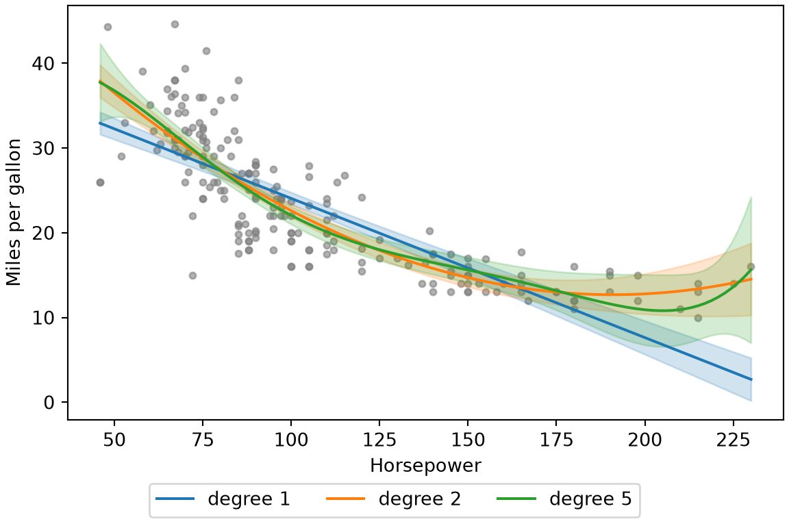
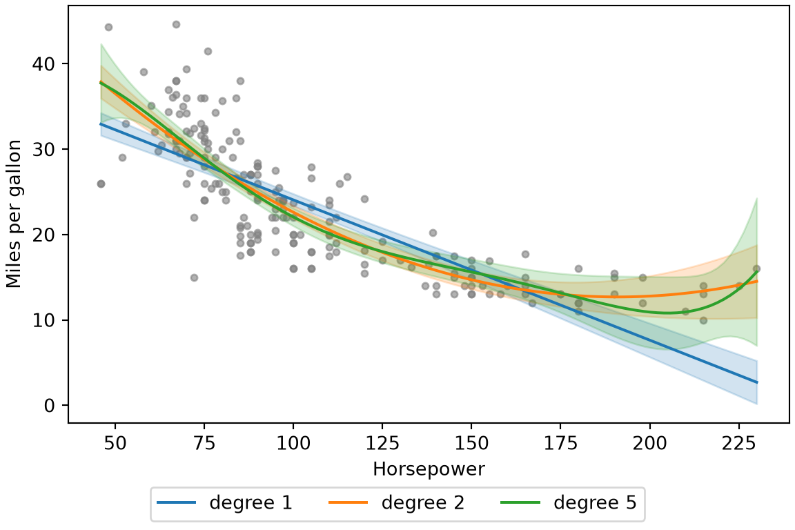
2. The test sRMSE is 4.80 miles per gallon for degree \(1\) (95% interval 4.24 to 5.29), 4.18 for degree \(2\) (3.60 to 4.68) and 4.14 for degree \(5\) (3.56 to 4.64). Each interval is a 95% \(t\) interval for the mean of the \(196\) squared errors on the test cars, with its endpoints square-rooted, so it reflects which test cars were drawn, with the fitted curve held fixed.

ExrExercise 13 (Lab: a curve, and a held-out check (part 3))

Exercise 13 (Lab: a curve, and a held-out check (part 3)) Use the setup of Exercise 11.

Plot the three fitted curves over a scatter plot of the test cars.

Solution 13.

Show code
import matplotlib.pyplot as plt
import numpy as np
import pandas as pd
import statsmodels.api as sm

hp_grid = pd.Series(np.linspace(Auto["horsepower"].min(), Auto["horsepower"].max(), 100))
fig, ax = plt.subplots(figsize=(6, 4), layout="constrained")
ax.scatter(Auto["horsepower"][~auto_train], mpg[~auto_train], s=12, alpha=0.6, color="gray");
for degree in [1, 2, 5]:
    X_poly = poly_design(Auto["horsepower"], degree)
    poly_results = sm.OLS(mpg[auto_train], X_poly[auto_train]).fit()
    grid_design = poly_design(hp_grid, degree)
    # The band is the 95% confidence interval for the mean mpg at each horsepower
    band = poly_results.get_prediction(grid_design).conf_int(alpha=0.05)
    (line,) = ax.plot(hp_grid, poly_results.predict(grid_design), label=f"degree {degree}")
    ax.fill_between(hp_grid, band[:, 0], band[:, 1], color=line.get_color(), alpha=0.2);
ax.set_xlabel("Horsepower");
ax.set_ylabel("Miles per gallon");
fig.legend(loc="outside lower center", ncol=3);
plt.show()
Show code
grid = np.linspace(horsepower.min(), horsepower.max(), 100)
fig, ax = plt.subplots(figsize=(6, 4), layout="constrained")
ax.scatter(horsepower[test], y[test], s=12, alpha=0.6, color="gray");
for degree in [1, 2, 5]:
    Phi = np.column_stack([horsepower ** k for k in range(degree + 1)])
    beta_hat = np.linalg.lstsq(Phi[train], y[train], rcond=None)[0]
    Phi_grid = np.column_stack([grid ** k for k in range(degree + 1)])
    # The band is the 95% confidence interval for the mean mpg at each horsepower,
    # from the fit to the training cars
    band_lower, band_upper = mean_ci(beta_hat, Phi[train], Phi_grid, y_obs=y[train])
    (line,) = ax.plot(grid, Phi_grid @ beta_hat, label=f"degree {degree}")
    ax.fill_between(grid, band_lower, band_upper, color=line.get_color(), alpha=0.2);
ax.set_xlabel("Horsepower");
ax.set_ylabel("Miles per gallon");
fig.legend(loc="outside lower center", ncol=3);
plt.show()
Show code
library(tidymodels)

# The bands are the 95% confidence intervals
# for the mean mpg at each horsepower
hp_grid <- tibble(horsepower = seq(min(auto$horsepower),
                                   max(auto$horsepower)))
curves <- map(c(1, 2, 5), \(degree) {
  model <- poly_fit(degree)
  bind_cols(hp_grid,
            predict(model, new_data = hp_grid),
            predict(model, new_data = hp_grid, type = "conf_int"),
            degree = factor(degree))
}) |>
  list_rbind()
ggplot() +
  geom_point(data = auto_test, aes(horsepower, mpg),
             colour = "grey50", alpha = 0.6) +
  geom_ribbon(data = curves,
              aes(horsepower, ymin = .pred_lower, ymax = .pred_upper,
                  fill = degree),
              alpha = 0.2) +
  geom_line(data = curves, aes(horsepower, .pred, colour = degree),
            linewidth = 1) +
  labs(x = "Horsepower", y = "Miles per gallon",
       colour = "Degree", fill = "Degree")
Show code
library(ggplot2)

test_cars <- dplyr::filter(auto, !train)
grid <- tibble::tibble(
  horsepower = seq(min(auto$horsepower), max(auto$horsepower), length.out = 100)
)
train_cars <- dplyr::filter(auto, train)
# The bands are the 95% confidence intervals
# for the mean mpg at each horsepower
poly_curves <- c(1, 2, 5) |>
  lapply(function(degree) {
    model <- lm(mpg ~ poly(horsepower, degree, raw = TRUE), data = train_cars)
    fit_band <- predict(model, grid, interval = "confidence")
    tibble::tibble(grid, mpg = fit_band[, "fit"],
                   lower = fit_band[, "lwr"], upper = fit_band[, "upr"],
                   degree = factor(degree))
  }) |>
  dplyr::bind_rows()
ggplot(test_cars, aes(horsepower, mpg)) +
  geom_point(colour = "grey50", alpha = 0.6) +
  geom_ribbon(data = poly_curves,
              aes(ymin = lower, ymax = upper, fill = degree),
              alpha = 0.2) +
  geom_line(data = poly_curves, aes(colour = degree), linewidth = 1) +
  labs(x = "Horsepower", y = "Miles per gallon",
       colour = "Degree", fill = "Degree")
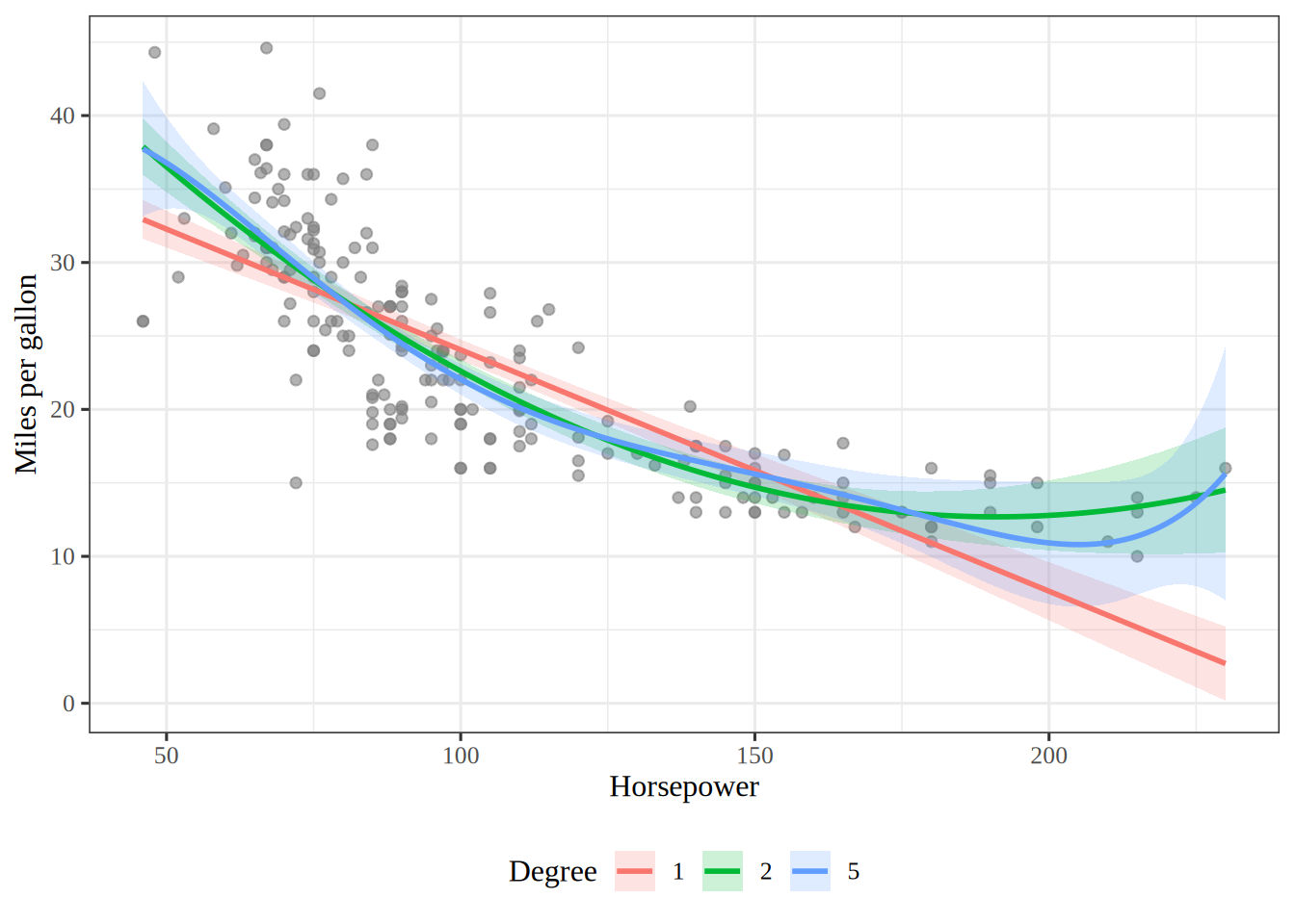
Figure 2: Miles per gallon against horsepower for the test cars, with a straight line, a bent curve and a degree-5 curve, each inside a shaded band.

3. The shaded bands in Figure 2 are 95% confidence intervals for the mean mpg at each horsepower, from the fit to the training cars.

ExrExercise 14 (Lab: a curve, and a held-out check (part 4))

Exercise 14 (Lab: a curve, and a held-out check (part 4)) Use the setup of Exercise 11.

Which degree would you choose?

Solution 14. Going from degree \(1\) to degree \(2\) lowers both errors by a lot. Going from degree \(2\) to degree \(5\) lowers both only slightly. Degree \(2\) gets nearly all of the gain with \(3\) coefficients, so it is the natural choice here.

ExrExercise 15 (Lab: a curve, and a held-out check (part 5))

Exercise 15 (Lab: a curve, and a held-out check (part 5)) Use the setup of Exercise 11.

What does the comparison of the two error columns show that the training error alone does not?

Solution 15. The training error always falls as the degree rises, as in Solution 6, so a small fall is weak evidence for the extra terms. The test error is the honest column, because we did not use those cars to choose the coefficients. The intervals all overlap, but the same test cars score every degree, so the three errors move together, and an overlap would not show that the degrees tie. Here every test error is smaller than its training error. The usual order is the reverse, and a split like this one shows that one split is a noisy estimate: a different split can give a different order. Measuring that gap, and choosing a model by test error, is the subject of Generalization.

ExrExercise 16 (Lab: use a category as a feature)

Exercise 16 (Lab: use a category as a feature) The origin column codes where each car was made: \(1\) for American, \(2\) for European and \(3\) for Japanese. The numbers are labels, and not amounts, so a column of \(1\), \(2\) and \(3\) would be wrong as a feature.

Build two indicator columns, one that is \(1\) for European cars and one that is \(1\) for Japanese cars. Fit mpg on these two columns alone.

Solution 16.

import pandas as pd
import statsmodels.api as sm

place = Auto["origin"].map({1: "American", 2: "European", 3: "Japanese"})
# drop_first drops "American", the first level, which becomes the baseline
origin_columns = pd.get_dummies(place, drop_first=True, dtype=float)

auto_origin = sm.OLS(mpg, sm.add_constant(origin_columns)).fit()
# Each coefficient with its 95% confidence interval
print(pd.concat([auto_origin.params, auto_origin.conf_int()], axis=1)
      .set_axis(["coef", "lower", "upper"], axis=1))
               coef      lower      upper
const     20.033469  19.230049  20.836890
European   7.569472   5.845776   9.293167
Japanese  10.417164   8.790110  12.044217
origin = Auto["origin"].to_numpy()
european = (origin == 2).astype(float)
japanese = (origin == 3).astype(float)

beta_origin, Phi_origin = fit([european, japanese])
print(np.column_stack([beta_origin, coef_ci(beta_origin, Phi_origin)]))
[[20.03346939 19.23004902 20.83688976]
 [ 7.56947179  5.84577627  9.2931673 ]
 [10.41716352  8.79011016 12.04421689]]
library(tidymodels)

auto_origin <- auto |>
  mutate(origin = factor(origin, levels = 1:3,
                         labels = c("American", "European", "Japanese")))

origin_recipe <- recipe(mpg ~ origin, data = auto_origin) |>
  step_dummy(origin)
tm_origin <- workflow() |>
  add_recipe(origin_recipe) |>
  add_model(lm_spec) |>
  fit(auto_origin)

# Each coefficient with its 95% confidence interval
tidy(tm_origin, conf.int = TRUE)
fit_origin <- lm(mpg ~ factor(origin), data = auto)
# The table includes each coefficient's 95% confidence interval
parameters::parameters(fit_origin) |>
  parameters::print_md(digits = 4)
Parameter Coefficient SE 95% CI t(389) p
(Intercept) 20.0335 0.4086 (19.2300, 20.8369) 49.0247 < .001
origin (2) 7.5695 0.8767 (5.8458, 9.2932) 8.6339 < .001
origin (3) 10.4172 0.8276 (8.7901, 12.0442) 12.5878 < .001
Show code
coef_ci_origin <- py$coef_ci(py$beta_origin, py$Phi_origin)

1. The intercept is 20.0 (95% confidence interval 19.2 to 20.8), the average mpg of American cars, which have both indicators equal to \(0\). The European coefficient is 7.6 (5.8 to 9.3), the gap between the European and American averages, and the Japanese coefficient is 10.4 (8.8 to 12.0), the gap between the Japanese and American averages.

ExrExercise 17 (Lab: use a category as a feature (part 2))

Exercise 17 (Lab: use a category as a feature (part 2)) Use the setup of Exercise 16.

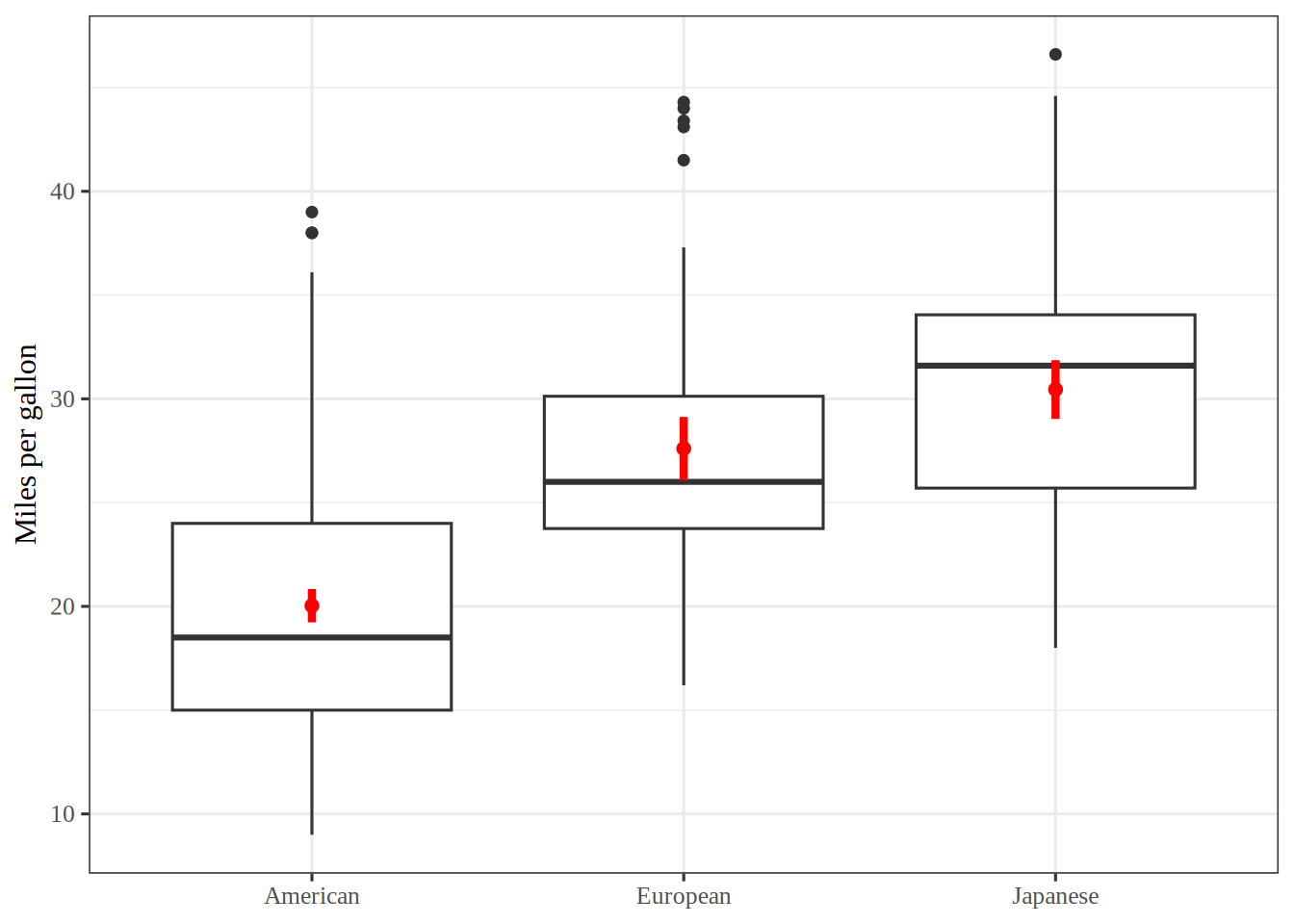
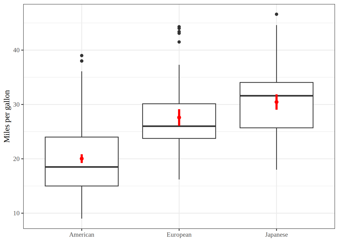
Draw side-by-side box plots of mpg for the three groups. Compute the sample mean mpg of each group. How do the sample means relate to the coefficients?

Solution 17.

Show code
groups = [Auto.loc[Auto["origin"] == k, "mpg"] for k in (1, 2, 3)]
positions = [1, 2, 3]
fig, ax = plt.subplots(figsize=(6, 4), layout="constrained")
_ = ax.boxplot(groups, tick_labels=["American", "European", "Japanese"])
# The averages and their intervals come from the model with the two indicator columns
ax.vlines(positions, group_lower, group_upper, color="C3", linewidth=3);
ax.plot(positions, group_means, "o", color="C3");
ax.set_ylabel("Miles per gallon");
plt.show()
Show code
library(tidymodels)

# One line from the lower to the upper end of each group's interval
interval_ends <- bind_rows(transmute(group_means, origin, mpg = .pred_lower),
                           transmute(group_means, origin, mpg = .pred_upper))
ggplot() +
  geom_boxplot(data = auto_origin, aes(origin, mpg)) +
  geom_line(data = interval_ends, aes(origin, mpg, group = origin),
            colour = "red", linewidth = 1.5) +
  geom_point(data = group_means, aes(origin, .pred), colour = "red", size = 2) +
  labs(x = NULL, y = "Miles per gallon")
Show code
library(ggplot2)

origin_labels <- c("American", "European", "Japanese")
group_means_plot <- data.frame(
  origin = factor(origin_labels, levels = origin_labels),
  group_means_base
)
# One line from the lower to the upper end of each group's interval
interval_ends <- rbind(
  data.frame(origin = group_means_plot$origin, mpg = group_means_plot$lwr),
  data.frame(origin = group_means_plot$origin, mpg = group_means_plot$upr)
)
ggplot() +
  geom_boxplot(data = auto, aes(factor(origin, labels = origin_labels), mpg)) +
  geom_line(data = interval_ends, aes(origin, mpg, group = origin),
            colour = "red", linewidth = 1.5) +
  geom_point(data = group_means_plot, aes(origin, fit),
             colour = "red", size = 2) +
  labs(x = NULL, y = "Miles per gallon")
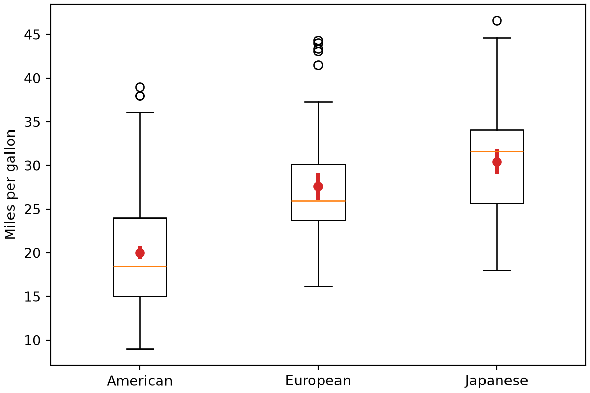
Figure 3: Miles per gallon for American, European and Japanese cars in the Auto data, with a red bar for each group.
print(mpg.groupby(place).mean())
origin
American    20.033469
European    27.602941
Japanese    30.450633
Name: mpg, dtype: float64
# The three group averages, each with a 95% confidence interval
group_rows = pd.DataFrame({"const": 1.0, "European": [0.0, 1.0, 0.0],
                           "Japanese": [0.0, 0.0, 1.0]})
print(auto_origin.get_prediction(group_rows).summary_frame(alpha=0.05)
      [["mean", "mean_ci_lower", "mean_ci_upper"]]
      .set_axis(["American", "European", "Japanese"]))
               mean  mean_ci_lower  mean_ci_upper
American  20.033469      19.230049      20.836890
European  27.602941      26.077936      29.127947
Japanese  30.450633      29.035777      31.865489
print(Auto.groupby("origin")["mpg"].mean())
origin
1    20.033469
2    27.602941
3    30.450633
Name: mpg, dtype: float64
# The three group averages, each with a 95% confidence interval
Phi_groups = np.array([[1, 0, 0], [1, 1, 0], [1, 0, 1]], float)
group_means = Phi_groups @ beta_origin
group_lower, group_upper = mean_ci(beta_origin, Phi_origin, Phi_groups)
print(np.column_stack([group_means, group_lower, group_upper]))
[[20.03346939 19.23004902 20.83688976]
 [27.60294118 26.07793562 29.12794673]
 [30.45063291 29.0357766  31.86548922]]

Three box plots of miles per gallon for American, European and Japanese cars. American cars have the lowest median, near 18.5. European and Japanese medians are higher, near 26 and 32, and the boxes for the three groups overlap partly. A red dot marks each group's average, with a short red vertical bar for its 95% confidence interval, which lies within the group's box.

auto_origin |> group_by(origin) |> summarise(mean_mpg = mean(mpg))
# The three group averages, each with a 95% confidence interval
origin_groups <- tibble(origin = factor(c("American", "European", "Japanese"),
                                        levels = levels(auto_origin$origin)))
group_means <- bind_cols(origin_groups,
                         predict(tm_origin, new_data = origin_groups),
                         predict(tm_origin, new_data = origin_groups,
                                 type = "conf_int"))
group_means

Drawn in R with ggplot2: three box plots of miles per gallon for American, European and Japanese cars. American cars have the lowest median, near 18.5. European and Japanese medians are higher, near 26 and 32, and the boxes for the three groups overlap partly. A red dot marks each group's average, with a short red vertical bar for its 95% confidence interval, which lies within the group's box.

tapply(auto$mpg, auto$origin, mean)
       1        2        3 
20.03347 27.60294 30.45063 
# The three group averages, each with a 95% confidence interval
origin_groups <- tibble::tibble(origin = 1:3)
group_means_base <- predict(fit_origin, origin_groups, interval = "confidence")
rownames(group_means_base) <- c("American", "European", "Japanese")
group_means_base
              fit      lwr      upr
American 20.03347 19.23005 20.83689
European 27.60294 26.07794 29.12795
Japanese 30.45063 29.03578 31.86549

Three box plots of miles per gallon for American, European and Japanese cars, drawn in R with ggplot2. American cars have the lowest median, near 18.5. European and Japanese medians are higher, near 26 and 32, and the boxes for the three groups overlap partly. A red dot marks each group's average, with a short red vertical bar for its 95% confidence interval, which lies within the group's box.

2. With only indicator columns, least squares reproduces the three group averages. Figure 3 shows the three group averages, each with its red bar. The red intervals in the figure are the 95% confidence intervals of those averages, and each coefficient’s interval is its \(t\) interval, the estimate plus or minus a \(t\) quantile times its standard error.

ExrExercise 18 (Lab: use a category as a feature (part 3))

Exercise 18 (Lab: use a category as a feature (part 3)) Use the setup of Exercise 16.

Add weight as a third column. What happens to the two origin coefficients, and why?

Solution 18.

X_origin_weight = sm.add_constant(pd.concat([Auto["weight"], origin_columns], axis=1))
auto_origin_weight = sm.OLS(mpg, X_origin_weight).fit()
print(pd.concat([auto_origin_weight.params, auto_origin_weight.conf_int()], axis=1)
      .set_axis(["coef", "lower", "upper"], axis=1))
               coef      lower      upper
const     43.732236  41.543128  45.921345
weight    -0.007027  -0.007656  -0.006398
European   0.970906  -0.324295   2.266106
Japanese   2.327150   1.020080   3.634220
beta_origin_weight, Phi_origin_weight = fit([weight, european, japanese])
print(np.column_stack([beta_origin_weight,
                       coef_ci(beta_origin_weight, Phi_origin_weight)]))
[[ 4.37322362e+01  4.15431276e+01  4.59213447e+01]
 [-7.02708331e-03 -7.65634196e-03 -6.39782466e-03]
 [ 9.70905585e-01 -3.24294839e-01  2.26610601e+00]
 [ 2.32714990e+00  1.02008022e+00  3.63421958e+00]]
origin_weight_recipe <- recipe(mpg ~ weight + origin, data = auto_origin) |>
  step_dummy(origin)
tm_origin_weight <- workflow() |>
  add_recipe(origin_weight_recipe) |>
  add_model(lm_spec) |>
  fit(auto_origin)
tidy(tm_origin_weight, conf.int = TRUE)
fit_origin_weight <- lm(mpg ~ weight + factor(origin), data = auto)
parameters::parameters(fit_origin_weight) |>
  parameters::print_md(digits = 4)
Parameter Coefficient SE 95% CI t(388) p
(Intercept) 43.7322 1.1134 (41.5431, 45.9213) 39.2771 < .001
weight -0.0070 0.0003 (-0.0077, -0.0064) -21.9559 < .001
origin (2) 0.9709 0.6588 (-0.3243, 2.2661) 1.4738 0.141
origin (3) 2.3271 0.6648 (1.0201, 3.6342) 3.5005 < .001
Show code
coef_ci_origin_weight <- py$coef_ci(py$beta_origin_weight, py$Phi_origin_weight)

3. With weight in the model, the origin coefficients become 1.0 (95% confidence interval -0.3 to 2.3) and 2.3 (1.0 to 3.6). They are now the gaps between cars of the same weight. American cars are heavier on average, so much of the raw gap was a weight gap, and it shrinks once weight is held fixed.

ExrExercise 19 (Lab: let the weight slope depend on a category)

Exercise 19 (Lab: let the weight slope depend on a category) Let american be the indicator that is \(1\) for American cars (origin \(= 1\)) and \(0\) for the rest. Fit mpg on weight, american and their interaction \(\text{weight} \times \text{american}\). What is the fitted change in mpg per \(1000\) pounds for American cars, and for other cars?

Solution 19.

import statsmodels.api as sm

X_american = sm.add_constant(Auto[["weight"]])
X_american["american"] = (Auto["origin"] == 1).astype(float)
X_american["weight:american"] = X_american["weight"] * X_american["american"]
auto_american = sm.OLS(mpg, X_american).fit()

# Each coefficient with its 95% confidence interval
print(pd.concat([auto_american.params, auto_american.conf_int()], axis=1)
      .set_axis(["coef", "lower", "upper"], axis=1))
                      coef      lower      upper
const            48.771246  44.871650  52.670842
weight           -0.008467  -0.010121  -0.006812
american         -5.622778 -10.173892  -1.071663
weight:american   0.001613  -0.000175   0.003400
# Per 1000 pounds, the slope is a linear combination of the coefficients,
# so t_test gives its 95% confidence interval
for label, weights_1000 in [("other", [0, 1000, 0, 0]), ("american", [0, 1000, 0, 1000])]:
    change = auto_american.t_test(np.array(weights_1000))
    print(label, change.effect[0], change.conf_int(alpha=0.05)[0])
other -8.46677756922959 [-10.12122921  -6.81232592]
american -6.853986380923989 [-7.53124225 -6.17673051]
american = (origin == 1).astype(float)
beta_american, Phi_american = fit([weight, american, weight * american])
print(np.column_stack([beta_american, coef_ci(beta_american, Phi_american)]))
[[ 4.87712463e+01  4.48716503e+01  5.26708424e+01]
 [-8.46677757e-03 -1.01212292e-02 -6.81232592e-03]
 [-5.62277783e+00 -1.01738925e+01 -1.07166317e+00]
 [ 1.61279119e-03 -1.74912859e-04  3.40049524e-03]]
# Per 1000 pounds, the slope is a linear combination c'beta of the coefficients
c_other = np.array([0, 1000, 0, 0])
c_american = np.array([0, 1000, 0, 1000])
slope_ci_other = contrast_ci(beta_american, Phi_american, c_other)
slope_ci_american = contrast_ci(beta_american, Phi_american, c_american)
print(c_other @ beta_american, slope_ci_other)
-8.466777569232235 (np.float64(-10.121229213739927), np.float64(-6.812325924724543))
print(c_american @ beta_american, slope_ci_american)
-6.853986380922909 (np.float64(-7.5312422523846685), np.float64(-6.17673050946115))
library(tidymodels)

auto_american <- auto |> mutate(american = as.numeric(origin == 1))
tm_american <- lm_spec |> fit(mpg ~ weight * american, data = auto_american)

# Each coefficient with its 95% confidence interval
tidy(tm_american, conf.int = TRUE)
# Per 1000 pounds, the slope is a linear combination of the coefficients,
# with the weights (0, 1000, 0, 0) for other cars
# and (0, 1000, 0, 1000) for American cars.
# lincomb_ci() is one of the interval helpers.
engine_american <- extract_fit_engine(tm_american)
bind_rows(
  other = as_tibble(as.list(lincomb_ci(engine_american, c(0, 1000, 0, 0)))),
  american = as_tibble(as.list(
    lincomb_ci(engine_american, c(0, 1000, 0, 1000))
  )),
  .id = "cars"
)
auto <- dplyr::mutate(auto, american = as.numeric(origin == 1))
fit_american <- lm(mpg ~ weight * american, data = auto)

# Each coefficient with its 95% confidence interval
parameters::parameters(fit_american) |>
  parameters::print_md(digits = 4)
Parameter Coefficient SE 95% CI t(388) p
(Intercept) 48.7712 1.9834 (44.8717, 52.6708) 24.5895 < .001
weight -0.0085 0.0008 (-0.0101, -0.0068) -10.0616 < .001
american -5.6228 2.3148 (-10.1739, -1.0717) -2.4291 0.016
weight × american 0.0016 0.0009 (-0.0002, 0.0034) 1.7737 0.077
# Per 1000 pounds, the slope is a linear combination of the coefficients,
# with the weights (0, 1000, 0, 0) for other cars
# and (0, 1000, 0, 1000) for American cars.
# lincomb_ci() is one of the interval helpers.
rbind(other = lincomb_ci(fit_american, c(0, 1000, 0, 0)),
      american = lincomb_ci(fit_american, c(0, 1000, 0, 1000)))
          estimate      lower     upper
other    -8.466778 -10.121229 -6.812326
american -6.853986  -7.531242 -6.176731

The model is \(\hat{y} = \hintcoef + \hcoef{1} w + \hcoef{2} a + \hcoef{3} \, w a\), where \(w\) is weight and \(a\) is the american indicator. For other cars, \(a = 0\), and the model is the line \(\hintcoef + \hcoef{1} w\). For American cars, \(a = 1\), and the model is the line \((\hintcoef + \hcoef{2}) + (\hcoef{1} + \hcoef{3}) w\). So the interaction gives each group its own intercept and its own slope.

Per \(1000\) pounds, the fitted change in mpg is -8.5 (95% confidence interval -10.1 to -6.8) for other cars and -6.9 (-7.5 to -6.2) for American cars. Each interval is a \(t\) interval for a linear combination of the coefficients, built from their estimated covariance matrix. Without the product column, the two lines would be parallel, as in part 3 of Exercise 16.

2 Concepts that the lab applies

The concepts that these exercises apply, such as interaction terms, confidence intervals for a coefficient, prediction intervals, and residual plots, are on the page Interactions, Inference and Diagnostics.

Back to top

References

[1]
G. James, D. Witten, T. Hastie, R. Tibshirani, and J. Taylor, An introduction to statistical learning: With applications in Python. Springer, 2023. doi: 10.1007/978-3-031-38747-0.