# The Python chunks on this page import these packages; reticulate provisions them.library(reticulate)library(tidymodels)# nolint: undesirable_function_linter
This material was a section of the logistic regression page. Its sources are credited in that page’s Source note.
The naive Bayes assumption and its Spambase example moved here from the probability page; they are adapted from Brian Hutchinson’s Fall 2024 DATA 471 probability refresher [1].
Exercise 1 (Classifying with Bayes’ rule) A logistic regression model gives \(\Pr[Y = k \mid \vX = \vx]\) directly. Suppose instead that the label has \(K\)classes and that we knew, for each class\(k = 1, \ldots, K\):
the class prior \(\pi_k = \Pr[Y = k]\), the probability of class \(k\) before the features are seen;
the class-conditional density \(f_k(\vx)\), the conditional density of the features given \(Y = k\).
Use Bayes’ rule to express \(\Pr[\Outvar = k \mid \vX = \vx]\) in terms of \(\pi_k\) and \(f_k\).
ExrExercise 2 (Classifying with Bayes’ rule (part 2))
Exercise 2 (Classifying with Bayes’ rule (part 2)) Use the setup of Exercise 1.
To classify \(\vx\), we select the class with the largest posterior probability. Which factor in your formula can be omitted when comparing classes, and why?
Solution 2. In the posterior formula of Solution 1, the denominator is the same for every \(k\), because it is the marginal density of \(\vX\), with the class summed out. At a point \(\vx\) where that density is positive, dividing every posterior by the same positive number does not change which posterior is largest. So the predicted class is
\[
\hy(\vx) = \argmax_k \; \pi_k f_k(\vx),
\]
and it is enough to compare the products \(\pi_k f_k(\vx)\).
ExrExercise 3 (Classifying with Bayes’ rule (part 3))
Exercise 3 (Classifying with Bayes’ rule (part 3)) Use the setup of Exercise 1.
Where would \(\pi_k\) and \(f_k\) come from in practice?
Solution 3. Both are estimated from the training data. The proportion of training points in class \(k\)estimates\(\pi_k\). Estimating \(f_k\)means choosing a family of densities for the features within a class and fitting it to the training points of that class. Each choice of family gives a different classifier. The rest of this section uses the multivariate normal family.
LemTheorem 1 (The posterior from a prior and class densities)
Theorem 1 (The posterior from a prior and class densities) Let class\(k\) have prior \(\pi_k > 0\) and feature density \(f_k(\vx)\), for \(k = 1, \dots, K\), and let \(\vx\) be a point where the marginal density \(\sumto{l}{K} \pi_l f_l(\vx)\) is greater than \(0\). Then
ExmExample 1 (A posterior from two class densities)
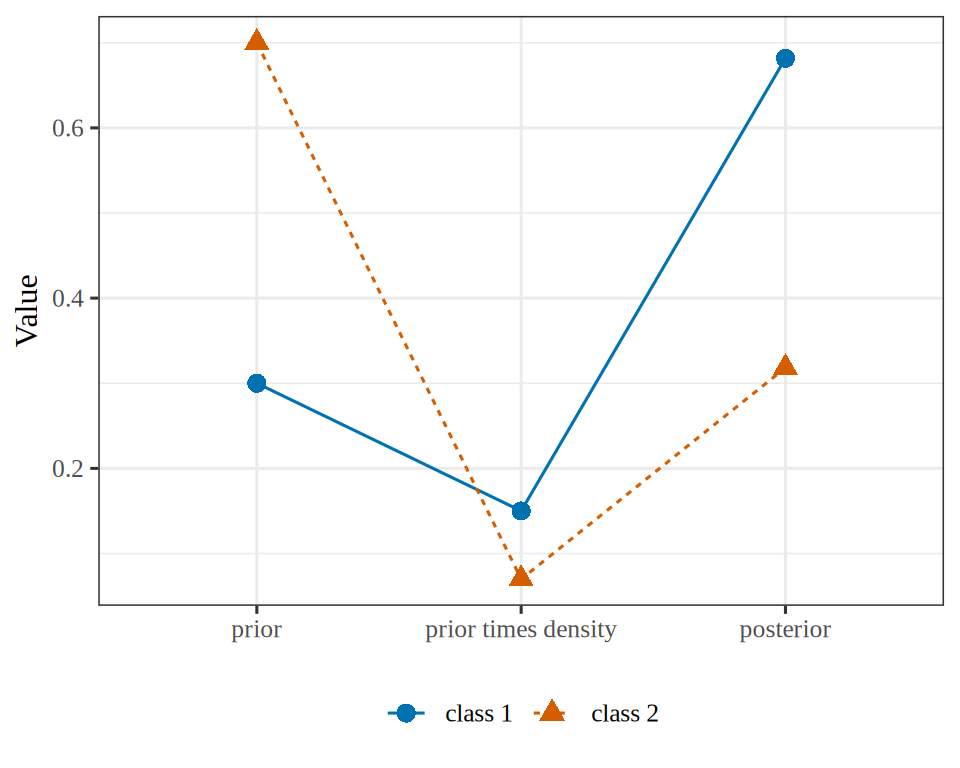
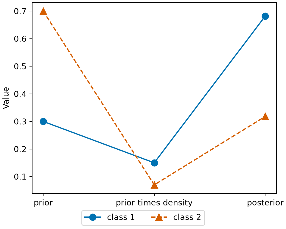
Example 1 (A posterior from two class densities) Two classes have priors \(\pi_1 = 0.3\) and \(\pi_2 = 0.7\), and at an observed \(\vx\) their class densities are \(f_1(\vx) = 0.5\) and \(f_2(\vx) = 0.1\). Find the posteriors and the class with the larger posterior.
The products are 0.15 and 0.07, so by Theorem 1 the posteriors are 0.682 and 0.318. Class 1 has the larger posterior, although class 2 has the larger prior.
Show code
library(ggplot2)bf_steps<-c("prior", "prior times density", "posterior")bf<-data.frame( step =factor(rep(bf_steps, each =2), levels =bf_steps), class =rep(c("class 1", "class 2"), times =3), value =c(br_prior, br_joint, br_post))ggplot(bf)+aes(step, value, colour =class, shape =class, linetype =class, group =class)+geom_line()+geom_point(size =3)+scale_colour_manual(values =c("class 1"="#0072B2", "class 2"="#D55E00"))+labs(x =NULL, y ="Value", colour =NULL, shape =NULL, linetype =NULL)
Figure 1: The prior, the prior times the density, and the posterior of the two classes of Example 1. Class 2 has the larger prior, but the density of class 1 is large enough at this observation that class 1 has the larger posterior.
Definition 1 (Bayes classifier) Let \(\pi_k\) and \(f_k\) be the true class priors and class-conditional densities of the features. The Bayes classifier assigns each \(\vx\) to the class with the largest posterior probability,
\[
\hy(\vx) = \argmax_k \; \pi_k f_k(\vx),
\]
as in Theorem 1. No classifier has a smaller probability of misclassifying a new observation [2, Ch. 2], [3].
ExmExample 2 (The Bayes classifier for two normal classes)
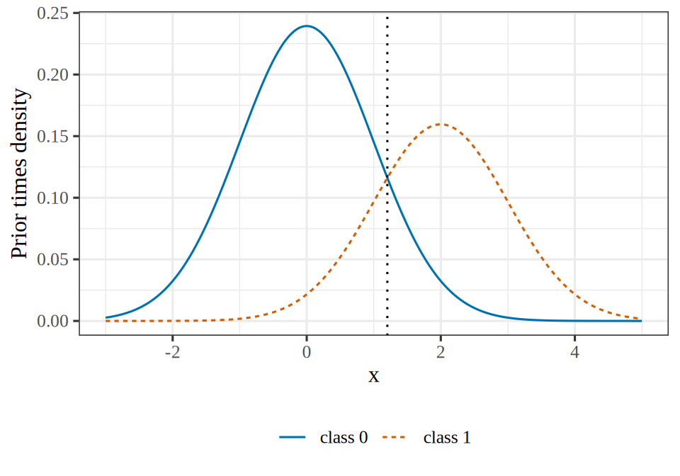
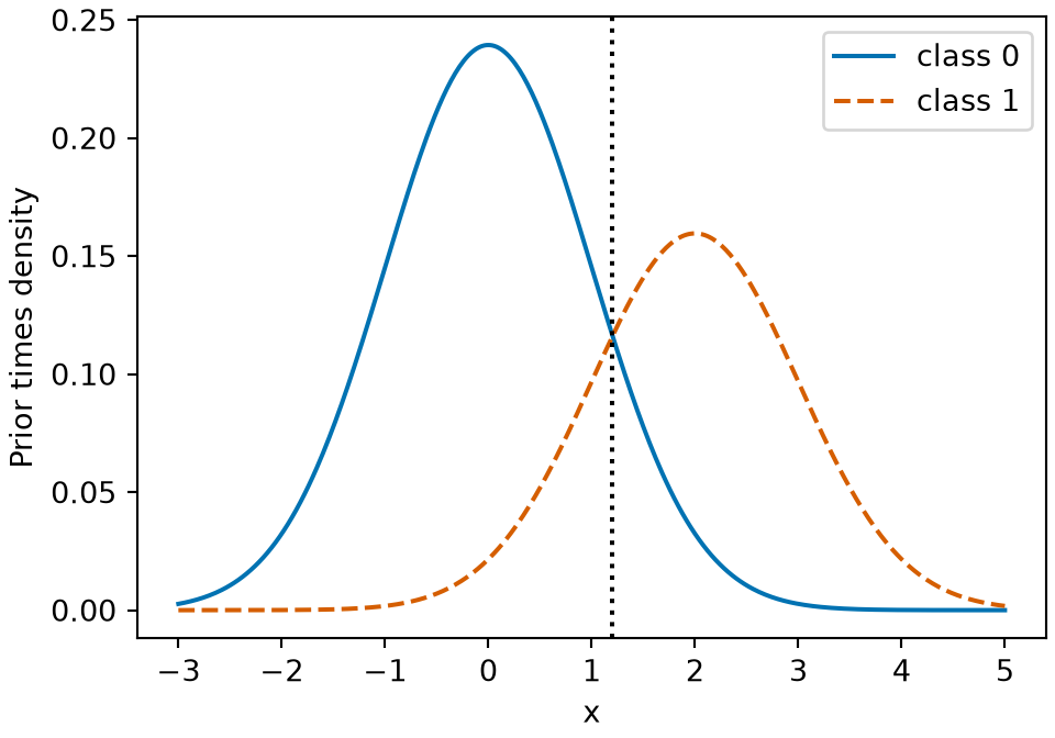
Example 2 (The Bayes classifier for two normal classes) Suppose that a single feature\(X\) is normal with mean\(0\) and variance\(1\) in class\(0\), and with mean \(2\) and variance \(1\) in class \(1\), and that the true priors are \(\pi_0 = 0.6\) and \(\pi_1 = 0.4\). Find the rule of the Bayes classifier and its probability of misclassifying a new observation.
The products \(\pi_0 f_0(x)\) and \(\pi_1 f_1(x)\) are equal at \(x =\) 1.203, so the Bayes classifier assigns class 0 to every \(x\) below 1.203 and class 1 to every \(x\) above it. The cut point is above the midpoint \(1\) of the two means, because class 0 has the larger prior. The classifier misclassifies a new observation with probability 0.154, and no other rule has a smaller probability for these two classes. Figure 2 plots the two products: the class-0 curve is higher to the left of the dotted cut line, and the class-1 curve is higher to its right.
Show code
# weight each class density by its prior, on a grid of feature valuesbc_x<-seq(-3, 5, length.out =401)bc_w0<-bc_prior[1]*dnorm(bc_x, bc_mean[1], 1)bc_w1<-bc_prior[2]*dnorm(bc_x, bc_mean[2], 1)bc_curves<-tibble::tibble(x =bc_x, `class 0` =bc_w0, `class 1` =bc_w1)|>tidyr::pivot_longer(-x, names_to ="class", values_to ="weighted")bc_colours<-c("class 0"="#0072B2", "class 1"="#D55E00")# the Bayes classifier switches class where the two curves crossbc_curves|>ggplot()+aes(x =x, y =weighted, colour =class, linetype =class)+geom_line()+geom_vline(xintercept =bc_cut, linetype ="dotted")+scale_colour_manual(values =bc_colours)+labs(x ="x", y ="Prior times density", colour =NULL, linetype =NULL)
Show code
import matplotlib.pyplot as plt# weight each class density by its prior, on a grid of feature valuesx_bc = np.linspace(-3, 5, 401)w0_bc = prior_bc[0] * norm.pdf(x_bc, mean_bc[0], 1)w1_bc = prior_bc[1] * norm.pdf(x_bc, mean_bc[1], 1)fig, ax = plt.subplots(figsize=(5, 3.5), layout="constrained")ax.plot(x_bc, w0_bc, color="#0072B2", linestyle="-", label="class 0");ax.plot(x_bc, w1_bc, color="#D55E00", linestyle="--", label="class 1");# the Bayes classifier switches class where the two curves crossax.axvline(cut_bc, color="black", linestyle=":");ax.set_xlabel("x");ax.set_ylabel("Prior times density");ax.legend();plt.show()
Figure 2: The joint density\(\dens(Y = k,\, X = x)\) of class\(k\) and the feature value \(x\), for each class \(k\) of Example 2, plotted against \(x\). The joint density equals\(\pi_k f_k(x)\), the class’s prior times the class’s density. The dotted line marks where the Bayes classifier switches classes.
Definition 2 (Generative classifier (plug-in Bayes classifier)) A generative classifier is a classifier built on a generative model. It models the joint distribution of the label and the features through a class prior \(\pi_k\) and a class-conditional density \(f_k(\vx)\) for each class \(k\), estimates both from training data[4], and classifies each \(\vx\) by the largest estimated posterior probability \[
\widehat{\Pr}[\Outvar = k \mid \vX = \vx] = \frac{\hat\pi_k \hf_k(\vx)}{\sumto{l}{K} \hat\pi_l \hf_l(\vx)},
\] the formula of Theorem 1 with the estimates \(\hat\pi_k\) and \(\hf_k\) in place of the true priors and densities. Because it puts estimates into the Bayes classifier, it is also called a plug-in Bayes classifier.
ExmExample 3 (A Gaussian generative classifier for the stock market)
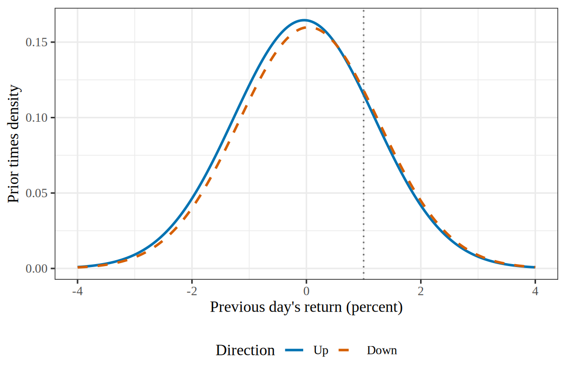
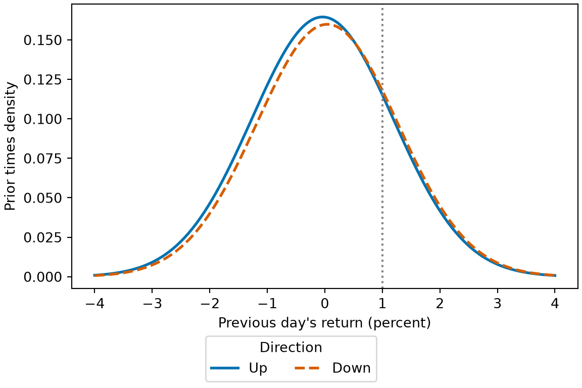
Example 3 (A Gaussian generative classifier for the stock market) Return to the Smarket data of the Smarket fit exercise. Model the previous day’s return, Lag1, within each direction as a Gaussian distribution, fitted to the days before 2005. Then classify a day whose previous return was \(1\%\).
           prior    mean      sd  posterior
Direction
Down       0.492  0.0428  1.2274     0.5059
Up         0.508 -0.0395  1.2317     0.4941
The classes are nearly balanced, with 50.8% of the training days up. The mean of Lag1 is -0.040 on days that went up and 0.043 on days that went down, and the standard deviations are 1.232 and 1.227, almost equal. A day that follows a \(1\%\) return has posterior probability 0.494 of going up, so the classifier predicts Down, with a posterior close to one half. The two class-conditional densities overlap almost completely, which is the same difficulty that the Smarket probabilities figure shows for logistic regression.
Show code
library(ggplot2)gcf_grid<-seq(-4, 4, length.out =241)gcf_curves<-do.call(rbind, lapply(names(class_mean), function(dir){data.frame( lag1 =gcf_grid, weighted =prior[[dir]]*dnorm(gcf_grid, class_mean[[dir]], class_sd[[dir]]), direction =dir)}))gcf_curves$direction<-factor(gcf_curves$direction, levels =c("Up", "Down"))ggplot(gcf_curves)+aes(lag1, weighted, colour =direction, linetype =direction)+geom_line(linewidth =0.9)+geom_vline(xintercept =x0, linetype ="dotted", colour ="grey40")+scale_colour_manual(values =c(Up ="#0072B2", Down ="#D55E00"))+scale_linetype_manual(values =c(Up ="solid", Down ="dashed"))+labs( x ="Previous day's return (percent)", y ="Prior times density", colour ="Direction", linetype ="Direction")
Figure 3: Each class’s prior times its density for the previous day’s return, from Example 3. At a return of \(1\%\) (dotted line) the two curves almost coincide, so the classifier cannot separate the classes.
RemarkRemark 2 (A discriminative classifier for the Smarket training days)
Remark 2 (A discriminative classifier for the Smarket training days). Logistic regression is a discriminative model: it models \(\Pr[Y = k \mid \vX = \vx]\) directly and does not model the distribution of the features. For comparison with Example 3, the code fits a logistic regression of the direction on Lag1 to the Smarkettraining days before 2005 and computes the probability of an up day after a \(1\%\) return.
disc_fit<-glm(I(Direction=="Up")~Lag1, family =binomial, data =da_train)disc_day<-tibble::tibble(Lag1 =x0)disc_prob<-predict(disc_fit, disc_day, type ="response")disc_coef<-coef(disc_fit)disc_out<-c(disc_coef, p_up =disc_prob[[1]])round(disc_out, 4)
(Intercept)        Lag1        p_up
     0.0322     -0.0546      0.4944
import statsmodels.api as smimport statsmodels.formula.api as smfda_train_py = da_train_py.assign(up=(da_train_py["Direction"] =="Up").astype(int))disc_py = smf.glm("up ~ Lag1", data=da_train_py, family=sm.families.Binomial()).fit()print(disc_py.params.round(4).to_dict())
The fitted model has an intercept and a slope, and nothing else: it has no prior, no classmean and no class variance, because it does not model how Lag1 is distributed. After a \(1\%\) return it gives an up day probability 0.4944, close to the 0.4941 of the generative classifier.
2 Linear discriminant analysis
ExrExercise 4 (Gaussian classes with one covariance matrix)
Exercise 4 (Gaussian classes with one covariance matrix) Let \(\vX \in \reals^{\ninputvars}\), and suppose that within class\(k\) the features are multivariate normal, \(\vX \mid Y = k \sim \ndist{\vm_k, \Sigma}\), with a mean\(\vm_k\) for each class and onecovariance matrix\(\Sigma\) shared by all of them. The density is
Solution 4. Assume that \(\Sigma\) is positive definite and every \(\pi_k > 0\). Then \(\inv{\Sigma}\) exists, because a positive definite matrix is invertible, and \(\abs{\Sigma} > 0\), so \(\log\abs{\Sigma}\) is defined. Every normal density is positive, so every product \(\pi_k f_k(\vx)\) is positive and has a logarithm. Write \(q_k(\vx) = \tp{(\vx - \vm_k)} \inv{\Sigma} (\vx - \vm_k)\) for the quadratic form. Taking the logarithm of the product turns it into a sum:
\[
\begin{aligned}
\log\paren{\pi_k f_k(\vx)}
&= \log \pi_k + \log f_k(\vx)
&& \text{(log of a product)} \\
&= \log \pi_k + \log\paren{\frac{1}{(2\pi)^{\ninputvars/2} \abs{\Sigma}^{1/2}} \expt\paren{-\frac12 q_k(\vx)}}
&& \text{(the Gaussian density)} \\
&= \log \pi_k + \log\frac{1}{(2\pi)^{\ninputvars/2} \abs{\Sigma}^{1/2}} + \log \expt\paren{-\frac12 q_k(\vx)}
&& \text{(log of a product)} \\
&= \log \pi_k - \log\paren{(2\pi)^{\ninputvars/2} \abs{\Sigma}^{1/2}} + \log \expt\paren{-\frac12 q_k(\vx)}
&& \text{(log of a reciprocal)} \\
&= \log \pi_k - \log\paren{(2\pi)^{\ninputvars/2} \abs{\Sigma}^{1/2}} - \frac12 q_k(\vx)
&& \text{(log of an exponential)} \\
&= \log \pi_k - \log (2\pi)^{\ninputvars/2} - \log \abs{\Sigma}^{1/2} - \frac12 q_k(\vx)
&& \text{(log of a product)} \\
&= \log \pi_k - \frac{\ninputvars}{2}\log(2\pi) - \frac12 \log\abs{\Sigma} - \frac12 q_k(\vx)
&& \text{(log of a power)}.
\end{aligned}
\]
Next, expand the quadratic form. Because \(\inv{\Sigma}\) is symmetric, the two cross terms are equal: \(\tp{\vm_k}\inv{\Sigma}\vx = \tp{\vx}\inv{\Sigma}\vm_k\).
ExrExercise 5 (Gaussian classes with one covariance matrix (part 2))
Exercise 5 (Gaussian classes with one covariance matrix (part 2)) Use the setup of Exercise 4.
Drop every term that is the same for all classes, and denote the remaining expression by \(\delta_k(\vx)\). Why does dropping those terms preserve \(\argmax_k \pi_k f_k(\vx)\)?
Solution 5. Three terms, \(-\frac{\ninputvars}{2}\log(2\pi)\), \(-\frac12 \log\abs{\Sigma}\) and \(-\frac12 \tp{\vx} \inv{\Sigma} \vx\), do not depend on \(k\). Adding the same number to every class’s score does not change which score is largest, so they can be dropped. The score that remains is
Solution 6. Yes: \(\delta_k(\vx)\) is an affine function of \(\vx\). The quadratic term \(\tp{\vx}\inv{\Sigma}\vx\) is the same in every class and was dropped, which is possible only because the covariance matrix is shared. What remains is the dot product of \(\vx\) with the fixed vector \(\inv{\Sigma}\vm_k\), plus the term \(-\frac12 \tp{\vm_k} \inv{\Sigma} \vm_k + \log \pi_k\), which does not depend on \(\vx\). The “linear” in linear discriminant analysis refers to this affine form, whose decision boundaries are hyperplanes.
Definition 3 (Linear discriminant function) For class\(k\) with prior\(\pi_k\) and mean\(\vm_k\), and a covariance matrix\(\Sigma\) shared by all classes, the linear discriminant function is
ExmExample 4 (The linear discriminant function with one feature)
Example 4 (The linear discriminant function with one feature) Let \(\ninputvars = 1\), with classmeans\(\vm_0 = 0\) and \(\vm_1 = 2\), shared variance\(\Sigma = 1\), and priors\(\pi_0 = 0.6\) and \(\pi_1 = 0.4\). Evaluate the linear discriminant function of each class at \(\vx = 1.2\).
Each \(\delta_k\) is an affine function of \(\vx\). More precisely, \(\log\paren{\pi_k f_k(\vx)} = \delta_k(\vx) + c(\vx)\), where \(c(\vx) = -\frac{\ninputvars}{2}\log(2\pi) - \frac12 \log\abs{\Sigma} - \frac12 \tp{\vx} \inv{\Sigma} \vx\) is the same for every class.
ExmExample 5 (The linear discriminant with one feature)
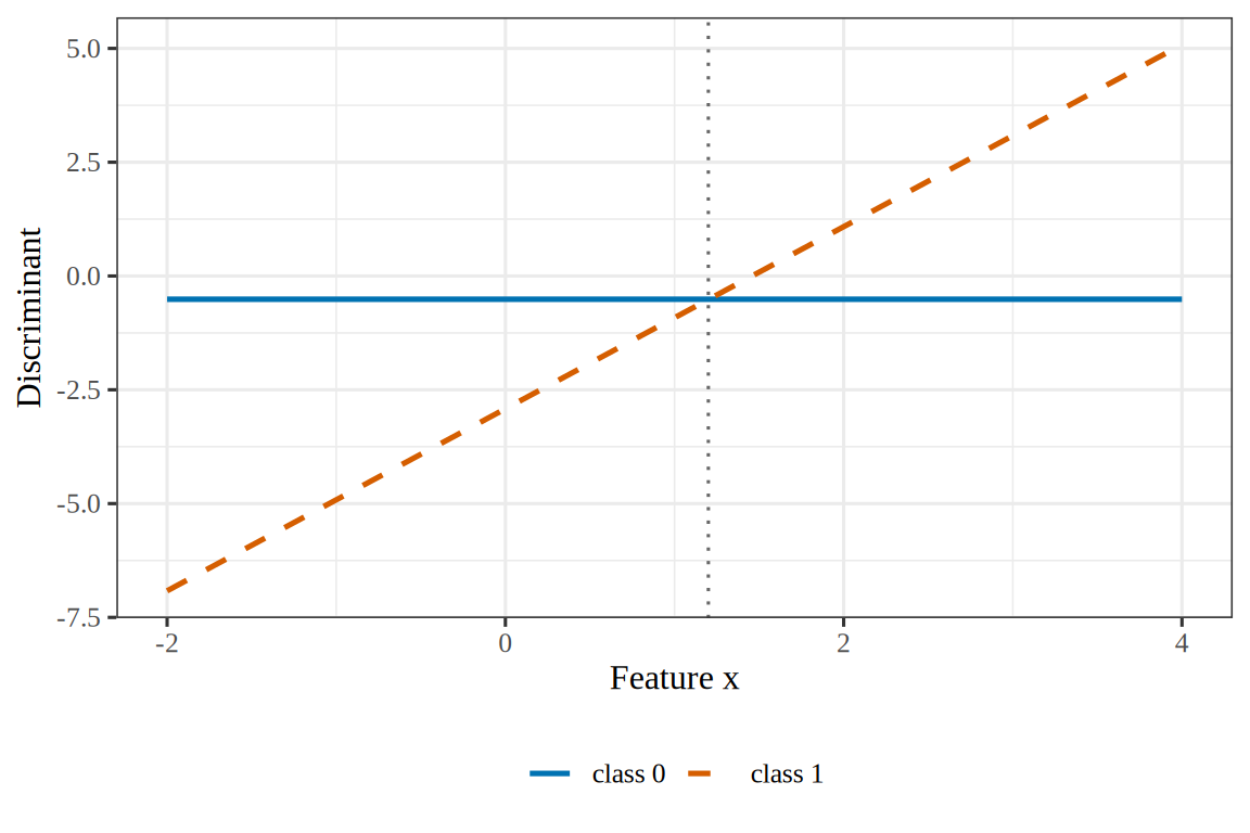
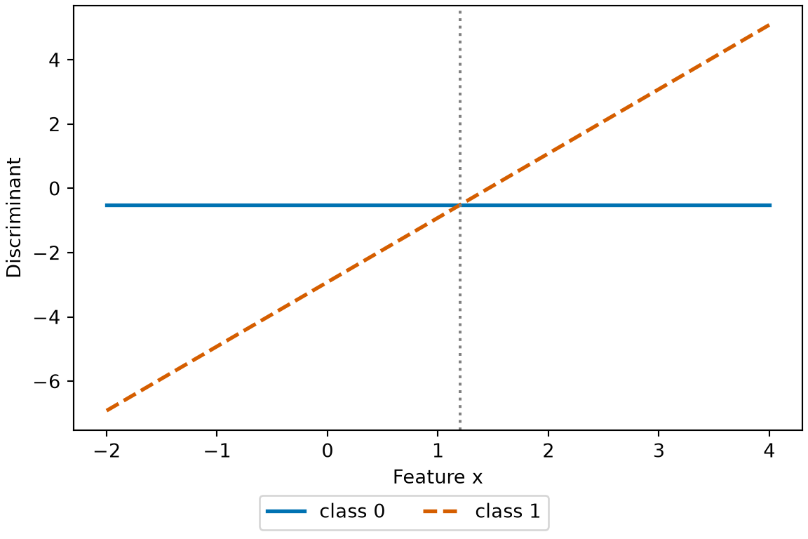
Example 5 (The linear discriminant with one feature) Let \(\ninputvars = 1\), with classmeans\(\vm_0 = 0\) and \(\vm_1 = 2\), shared variance\(\Sigma = 1\), and priors \(\pi_0 = 0.6\) and \(\pi_1 = 0.4\). Classify the point \(\vx = 1.2\).
The discriminants are -0.511 and -0.516, so Theorem 2 predicts class 0. The products \(\pi_k f_k(\vx)\), 0.1165 and 0.1159, give the same class, 0. The point is close to the boundary: the two discriminants differ by only 0.0055.
Figure 4: The linear discriminant functions of class \(0\) and class \(1\) plot as two straight-line graphs against the feature\(x\), and the point \(x = 1.2\) (dotted vertical line) is assigned to the class with the higher discriminant there (Example 5).
\(\hat{\vm}_k\), the average of the feature vectors in class \(k\);
\(\hSigma = \frac{1}{n - K}\sumkK \sum_{i : y_i = k} \soprod{\deviationv_i}\), the pooled within-class covariance matrix, where \(\deviationv_i \eqdef \devof{\vx_i}{\hat{\vm}_{y_i}}\) is the deviation of training point \(i\) from the average of its class.
Example 6 (LDA for one predictor) Fit LDA to the Smarket days before 2005 with Lag1 as the only predictor, so \(\ninputvars = 1\) and \(\Sigma\) is a single variance. Compute the pooled variance and the discriminant functions at \(x_0 = 1\) by hand, and compare the resulting posterior probabilities with a library’s.
The pooled variance is 1.512, between the two class variances 1.507 and 1.517. The two discriminant functions differ by only 0.022 at \(x_0\). The hand computation and the library give the same posteriors to four decimal places in both languages. With almost a thousand training days, dividing the pooled sum by \(n\) instead of \(n - K\) changes them only in the fifth decimal place. The posterior probability of Up is 0.4944, close to the 0.4941 of Example 3. The small difference from that example’s posterior comes from replacing the two class variances by their pool.
RemarkRemark 4 (The divisor of the pooled covariance matrix)
Remark 4 (The divisor of the pooled covariance matrix). The divisor \(n - K\) in Definition 4 makes \(\hSigma\) an unbiased estimator of \(\Sigma\). Within class\(k\), the sum of the outer products of the deviations from \(\hat{\vm}_k\) has expectation\((n_k - 1)\Sigma\), because estimating the class mean uses up one degree of freedom. Summing over the \(K\)classes gives expectation \((n - K)\Sigma\). The maximum likelihood estimator divides the same sum by \(n\) instead. Software differs: R’s MASS::lda() divides by \(n - K\)[7, Ch. 12]. scikit-learn’s LinearDiscriminantAnalysis depends on its solver and version. Its lsqr and eigen solvers divide by \(n\) in versions 1.8.0 and 1.9.1. Its default svd solver divides by \(n - K\) in version 1.8.0 and by \(n\) in version 1.9.1. With hundreds of training points the two choices give nearly the same classifier.
Remark 5 (Fisher’s linear discriminant). “Fisher’s linear discriminant” names a closely related method that finds the direction that best separates the class means, relative to the spread within the classes. In the two-class case its direction is proportional to the LDAcoefficient vector \(\inv{\Sigma}(\vm_1 - \vm_0)\)[8, Sec. 4.3.3].
Exercise 7 (The log odds of LDA) Consider two classes, \(Y \in \set{0, 1}\), under the LDA model. Compare with the log-odds exercise, where the log odds were assumedlinear.
Express \(\log \frac{\Pr[\Outvar = 1 \mid \vX = \vx]}{\Pr[\Outvar = 0 \mid \vX = \vx]}\) in terms of the linear discriminant functions\(\delta_1\) and \(\delta_0\).
Solution 7. Both posteriors share the denominator \(\sum_l \pi_l f_l(\vx)\) of Theorem 1, which cancels in their ratio. By Theorem 2, \(\log\paren{\pi_k f_k(\vx)} = \delta_k(\vx) + c(\vx)\), where \(c(\vx)\) collects the terms that the theorem drops and is the same for both classes. So
The last step uses the symmetry of \(\inv{\Sigma}\): expanding \(\tp{(\vm_1 + \vm_0)} \inv{\Sigma} (\vm_1 - \vm_0)\) gives four terms, and the cross terms \(-\tp{\vm_1}\inv{\Sigma}\vm_0\) and \(\tp{\vm_0}\inv{\Sigma}\vm_1\) are equal and opposite, so they cancel. Because \(\inv{\Sigma}\) is symmetric, \(\tp{\vx} \inv{\Sigma} (\vm_1 - \vm_0)\) is the dot product of \(\vx\) with \(\inv{\Sigma}(\vm_1 - \vm_0)\). So the log odds have the form \(\coef{0} + \dprod{\vcoef}{\vx}\), with
ExmExample 7 (LDA and logistic regression on the same days)
Example 7 (LDA and logistic regression on the same days) For the one-predictor LDA fit of Example 6, compute \(\coef{0}\) and \(\coef{1}\) from Theorem 3, and compare them with the coefficients of a logistic regression of Up on Lag1 fitted to the same days.
b1<-(class_mean[["Up"]]-class_mean[["Down"]])/pooledmid<-(class_mean[["Up"]]+class_mean[["Down"]])/2b0<-log(prior[["Up"]]/prior[["Down"]])-mid*b1logit_fit<-glm(I(Direction=="Up")~Lag1, family =binomial, data =da_train)lda_coef<-c(b0, b1)logit_coef<-coef(logit_fit)# nolint start: undesirable_function_linter. A matrix.rbind(LDA =lda_coef, logistic =logit_coef)|>round(4)
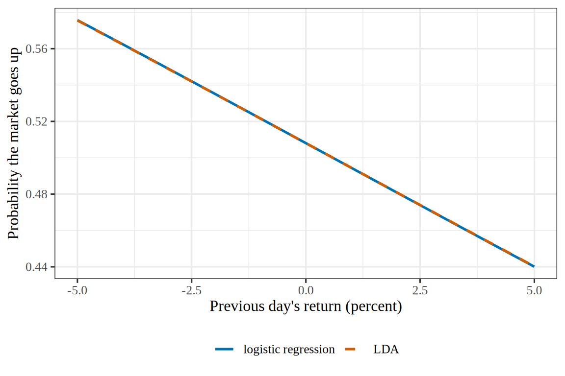
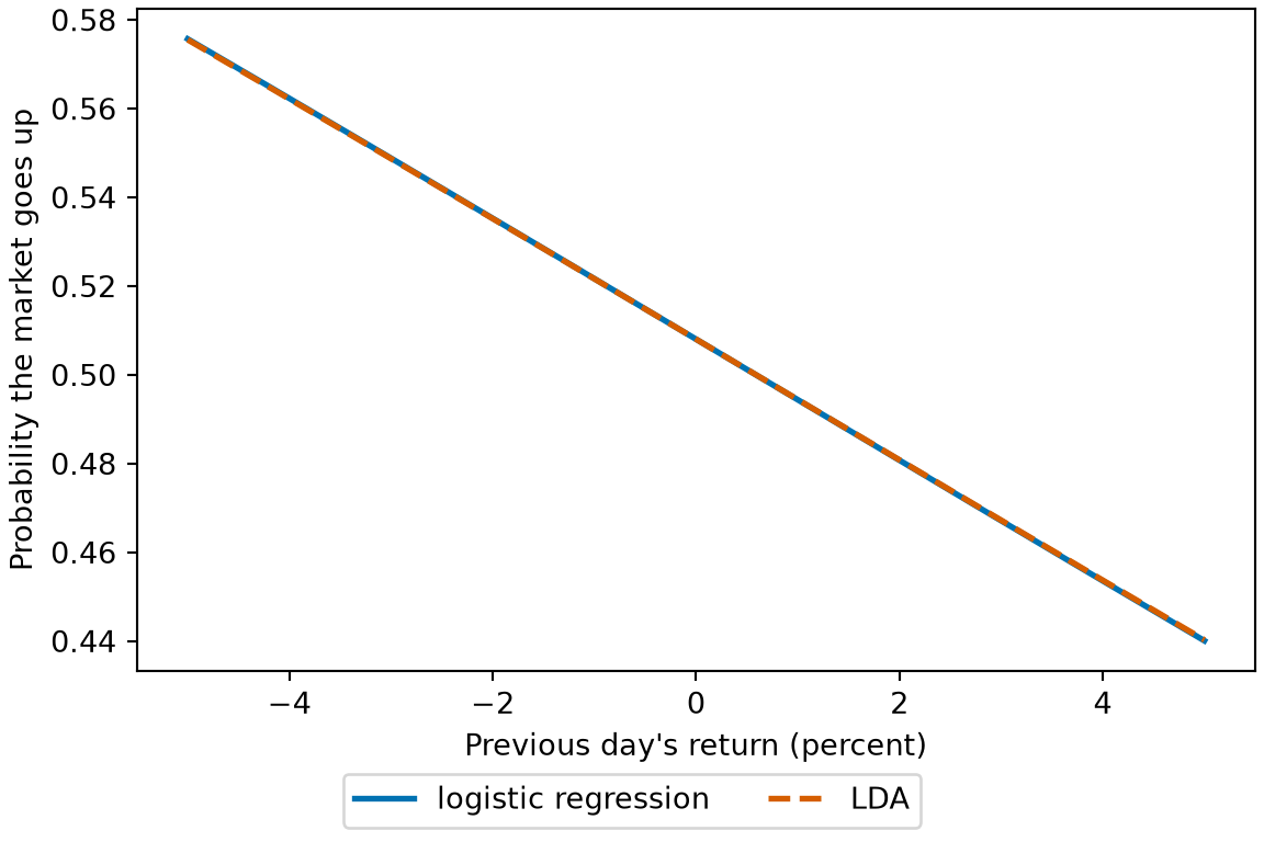
The two fittedlog-odds lines nearly coincide. LDA gives a slope of -0.0545 and logistic regression -0.0546, a difference of 0.3% of the logistic slope, and the intercepts are 0.0322 and 0.0322. Both slopes are negative and small: a rise of one percentage point in the previous day’s return lowers the log odds of an up day by about 0.05. When the class densities are normal with a shared variance, which is the model LDA assumes, the two methods’ estimates converge to the same coefficients as the sample grows [8, Sec. 4.4.5]. Their estimates can differ more when that model fails, for example for a strongly skewed predictor.
Show code
library(ggplot2)llo_grid<-seq(-5, 5, length.out =201)llo_curves<-data.frame( lag1 =rep(llo_grid, 2), prob =c(plogis(b0+b1*llo_grid), plogis(coef(logit_fit)[[1]]+coef(logit_fit)[[2]]*llo_grid)), model =rep(c("LDA", "logistic regression"), each =length(llo_grid)))llo_curves$model<-factor(llo_curves$model, levels =c("logistic regression", "LDA"))ggplot(llo_curves)+aes(lag1, prob, colour =model, linetype =model)+geom_line(linewidth =0.9)+scale_colour_manual(values =c("logistic regression"="#0072B2", LDA ="#D55E00"))+scale_linetype_manual(values =c("logistic regression"="solid", LDA ="dashed"))+labs( x ="Previous day's return (percent)", y ="Probability the market goes up", colour =NULL, linetype =NULL)
DatasetDataset 1: The credit-card default (Default) data
Dataset 1: The credit-card default (Default) data
Simulated records of 10000 credit-card holders, each saying whether the card holder defaulted on their debt, make up the Default data [2, Sec. 4.1]. The records describe no actual card holders. They are in data/default.csv, one line per card holder, copied from ISLR2, the R package of An Introduction to Statistical Learning[2]. Each line gives:
default: the outcome, Yes for a card holder who defaulted and No otherwise.
student: Yes for a student and No otherwise.
balance: the average balance left on the card after the monthly payment, in dollars.
import pandas as pdpd.set_option("display.max_columns", None)pd.set_option("display.width", 120)default_preview = pd.read_csv("data/default.csv")default_preview
     default student      balance        income
0         No      No   729.526495  44361.625074
1         No     Yes   817.180407  12106.134700
2         No      No  1073.549164  31767.138947
3         No      No   529.250605  35704.493935
4         No      No   785.655883  38463.495879
...      ...     ...          ...           ...
9995      No      No   711.555020  52992.378914
9996      No      No   757.962918  19660.721768
9997      No      No   845.411989  58636.156984
9998      No      No  1569.009053  36669.112365
9999      No     Yes   200.922183  16862.952321

[10000 rows x 4 columns]
dflt<-readr::read_csv("data/default.csv", show_col_types =FALSE)dflt_stats<-dflt|>dplyr::group_by(default)|>dplyr::summarise(n =dplyr::n(), mean =mean(balance), var =var(balance))dflt_n<-sum(dflt_stats$n)dflt_prior<-dflt_stats$n/dflt_nnames(dflt_prior)<-dflt_stats$defaultdflt_mean<-dflt_stats$meannames(dflt_mean)<-dflt_stats$defaultdflt_class_sd<-sqrt(dflt_stats$var)names(dflt_class_sd)<-dflt_stats$defaultdflt_ss<-(dflt_stats$n-1)*dflt_stats$vardflt_pooled<-sum(dflt_ss)/(dflt_n-2)dflt_sd<-sqrt(dflt_pooled)dflt_b1<-(dflt_mean[["Yes"]]-dflt_mean[["No"]])/dflt_pooleddflt_mid<-(dflt_mean[["Yes"]]+dflt_mean[["No"]])/2dflt_log_prior_ratio<-log(dflt_prior[["Yes"]]/dflt_prior[["No"]])dflt_b0<-dflt_log_prior_ratio-dflt_mid*dflt_b1dflt_boundary<--dflt_b0/dflt_b1dflt_grid<-seq(0, 2700, by =10)# Prior times density, on the log scale, for each class.dflt_log_yes<-log(dflt_prior[["Yes"]])+dnorm(dflt_grid, dflt_mean[["Yes"]], dflt_sd, log =TRUE)dflt_log_no<-log(dflt_prior[["No"]])+dnorm(dflt_grid, dflt_mean[["No"]], dflt_sd, log =TRUE)# Bayes' rule: class 1's share of the two products.dflt_bayes<-1/(1+exp(dflt_log_no-dflt_log_yes))dflt_sigmoid<-plogis(dflt_b0+dflt_b1*dflt_grid)dflt_glm<-glm(I(default=="Yes")~balance, family =binomial, data =dflt)dflt_logit<-coef(dflt_glm)dflt_abs_gap<-abs(dflt_bayes-dflt_sigmoid)dflt_gap<-max(dflt_abs_gap)dflt_coef<-c(LDA =dflt_b1, logistic =dflt_logit[["balance"]])signif(dflt_coef, 3)
     LDA logistic
  0.0046   0.0055
import numpy as npimport pandas as pdimport statsmodels.api as smimport statsmodels.formula.api as smffrom scipy.stats import normfrom scipy.special import expitdflt_py = pd.read_csv("data/default.csv")by_class_py = dflt_py.groupby("default")["balance"]n_dflt_py = by_class_py.size()prior_dflt_py = n_dflt_py / n_dflt_py.sum()mean_dflt_py = by_class_py.mean()pooled_dflt_py = ((n_dflt_py -1) * by_class_py.var()).sum() / (n_dflt_py.sum() -2)sd_dflt_py = np.sqrt(pooled_dflt_py)b1_dflt_py = (mean_dflt_py["Yes"] - mean_dflt_py["No"]) / pooled_dflt_pymid_dflt_py = (mean_dflt_py["Yes"] + mean_dflt_py["No"]) /2b0_dflt_py = np.log(prior_dflt_py["Yes"] / prior_dflt_py["No"]) - mid_dflt_py * b1_dflt_pygrid_dflt_py = np.arange(0, 2701, 10)# Prior times density, on the log scale, for each class.log_yes_py = np.log(prior_dflt_py["Yes"]) + norm.logpdf(grid_dflt_py, mean_dflt_py["Yes"], sd_dflt_py)log_no_py = np.log(prior_dflt_py["No"]) + norm.logpdf(grid_dflt_py, mean_dflt_py["No"], sd_dflt_py)# Bayes' rule: class 1's share of the two products.bayes_dflt_py =1/ (1+ np.exp(log_no_py - log_yes_py))sigmoid_dflt_py = expit(b0_dflt_py + b1_dflt_py * grid_dflt_py)dflt_py = dflt_py.assign(yes=(dflt_py["default"] =="Yes").astype(int))glm_dflt_py = smf.glm("yes ~ balance", data=dflt_py, family=sm.families.Binomial()).fit()print("LDA slope: ", float(np.round(b1_dflt_py, 6)))
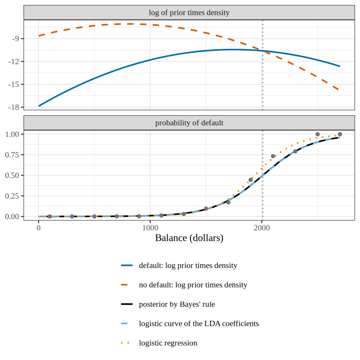
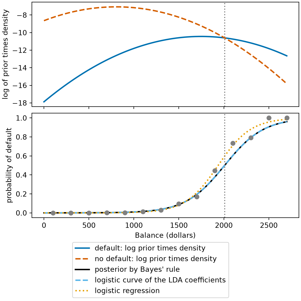
In Figure 6, the logarithm of the prior of each class times its density is a parabola in the balance \(\predvar\). The two parabolas have the same \(\predvar^2\) term, \(-\predvar^2 / (2 \Sigma)\), because the two classes share one variance\(\Sigma\), the single entry of the shared covariance matrix of Definition 4, which is \(1 \times 1\) here. Their difference, the log odds of default, is therefore an affine function of the balance, so the posterior from Bayes’ rule is the logistic curve of Theorem 3. On the grid the two curves differ by at most 9.4e-16, the size of floating-point rounding. The LDAcoefficient of balance is 0.0046 per dollar, and the posterior crosses one half at a balance of 2009 dollars. The small prior of default, 0.033, moves that crossing well above 1276 dollars, the midpoint of the two class means, where the two densities alone would cross. A logistic regressionfitted to the same card holders has the coefficient 0.0055, so its curve is steeper than LDA’s. The two fits differ because the balances do not follow LDA’s model: the sample standard deviations of balance are 341 dollars for the card holders who defaulted and 456 dollars for the others, not one shared value.
Show code
dflt_series<-c("default: log prior times density","no default: log prior times density","posterior by Bayes' rule","logistic curve of the LDA coefficients","logistic regression")dflt_panels<-c("log of prior times density", "probability of default")dflt_logit_eta<-dflt_logit[[1]]+dflt_logit[[2]]*dflt_griddflt_logit_curve<-plogis(dflt_logit_eta)dflt_n_grid<-length(dflt_grid)dflt_values<-c(dflt_log_yes, dflt_log_no, dflt_bayes, dflt_sigmoid, dflt_logit_curve)dflt_panel_of<-dflt_panels[c(1, 1, 2, 2, 2)]dflt_balance_col<-rep(dflt_grid, 5)dflt_series_col<-rep(dflt_series, each =dflt_n_grid)dflt_panel_col<-rep(dflt_panel_of, each =dflt_n_grid)dflt_curves<-tibble::tibble( balance =dflt_balance_col, value =dflt_values, series =dflt_series_col, panel =dflt_panel_col)dflt_curves$series<-factor(dflt_curves$series, levels =dflt_series)dflt_bins<-dflt|>dplyr::mutate(band =floor(balance/200)*200+100)|>dplyr::group_by(band)|>dplyr::summarise(value =mean(default=="Yes"), .groups ="drop")|>dplyr::mutate(panel =dflt_panels[[2]])dflt_colours<-c("#0072B2", "#D55E00", "black", "#56B4E9", "#E69F00")names(dflt_colours)<-dflt_seriesdflt_types<-c("solid", "dashed", "solid", "dashed", "dotted")names(dflt_types)<-dflt_seriesdflt_bin_aes<-ggplot2::aes(x =band, y =value)dflt_facets<-ggplot2::vars(panel)dflt_legend<-ggplot2::guide_legend(ncol =1)dflt_curves|>ggplot2::ggplot()+ggplot2::aes( x =balance, y =value, colour =series, linetype =series)+ggplot2::geom_line(linewidth =0.9)+ggplot2::geom_point( data =dflt_bins, mapping =dflt_bin_aes, inherit.aes =FALSE, colour ="grey45")+ggplot2::geom_vline( xintercept =dflt_boundary, linetype ="dotted", colour ="grey40")+ggplot2::facet_wrap(dflt_facets, ncol =1, scales ="free_y")+ggplot2::scale_colour_manual(values =dflt_colours)+ggplot2::scale_linetype_manual(values =dflt_types)+ggplot2::guides(colour =dflt_legend, linetype =dflt_legend)+ggplot2::labs( x ="Balance (dollars)", y =NULL, colour =NULL, linetype =NULL)+ggplot2::theme(legend.position ="bottom")
Show code
import matplotlib.pyplot as pltboundary_dflt_py =-b0_dflt_py / b1_dflt_pyband_py = np.floor(dflt_py["balance"] /200) *200+100rate_py = dflt_py.groupby(band_py)["yes"].mean()logit_curve_py = expit(glm_dflt_py.params["Intercept"] + glm_dflt_py.params["balance"] * grid_dflt_py)fig, (top, bottom) = plt.subplots(2, 1, figsize=(6, 6), sharex=True, layout="constrained")top.plot(grid_dflt_py, log_yes_py, color="#0072B2", linestyle="-", linewidth=2, label="default: log prior times density");top.plot(grid_dflt_py, log_no_py, color="#D55E00", linestyle="--", linewidth=2, label="no default: log prior times density");top.set_ylabel("log of prior times density");bottom.plot(grid_dflt_py, bayes_dflt_py, color="black", linestyle="-", linewidth=2, label="posterior by Bayes' rule");bottom.plot(grid_dflt_py, sigmoid_dflt_py, color="#56B4E9", linestyle="--", linewidth=2, label="logistic curve of the LDA coefficients");bottom.plot(grid_dflt_py, logit_curve_py, color="#E69F00", linestyle=":", linewidth=2, label="logistic regression");bottom.scatter(rate_py.index, rate_py.values, color="grey", zorder=3);bottom.set_ylabel("probability of default");bottom.set_xlabel("Balance (dollars)");for ax in (top, bottom): ax.axvline(boundary_dflt_py, color="grey", linestyle=":");fig.legend(loc="outside lower center", ncol=1);plt.show()
ExrExercise 10 (Same form, different fitting criterion)
Exercise 10 (Same form, different fitting criterion) By Theorem 3, two-class LDA and logistic regression give a posterior probability of the same functional form.
Each method chooses its parameters to maximize a likelihood. State the quantity LDA maximizes and the quantity logistic regression maximizes, in terms of \(\pi_k\), \(f_k\) and \(\Pr[\Outvar = 1 \mid \vX = \vx]\).
Solution 11. No: logistic log odds that are an affine function of \(\vx\) do not imply Gaussianclasses. Consider a single binary feature\(X \in \set{0, 1}\) with \(\Pr[X = 1 \mid Y = k] = q_k\), where \(0 < q_k < 1\). The class densities are \(f_k(x) = q_k^x (1 - q_k)^{1 - x}\) for \(x \in \set{0, 1}\), with logarithms\(\log f_k(x) = x \log q_k + (1 - x) \log(1 - q_k)\). By Theorem 1, the log odds of \(Y = 1\) are
\[
\begin{aligned}
\log \frac{\pi_1 f_1(x)}{\pi_0 f_0(x)}
&= \log\frac{\pi_1}{\pi_0} + \log f_1(x) - \log f_0(x)
&& \text{(log of a quotient of products)} \\
&= \log\frac{\pi_1}{\pi_0} + x \log q_1 + (1 - x) \log(1 - q_1) - x \log q_0 - (1 - x) \log(1 - q_0)
&& \text{(substitute $\log f_k(x)$)} \\
&= \log\frac{\pi_1}{\pi_0} + x \log\frac{q_1}{q_0} + (1 - x)\log\frac{1 - q_1}{1 - q_0}
&& \text{(log of a quotient)} \\
&= \log\frac{\pi_1}{\pi_0} + \log\frac{1 - q_1}{1 - q_0} + x \paren{\log\frac{q_1}{q_0} - \log\frac{1 - q_1}{1 - q_0}}
&& \text{(collect the terms in $x$)},
\end{aligned}
\]
which is an affine function of \(x\), although \(X\) is not Gaussian. Many other families of class-conditional densities also give log odds that are affine in \(\vx\), so logistic regression makes weaker distributional assumptions than LDA[8, Sec. 4.4.5].
ExrExercise 12 (Same form, different fitting criterion (part 3))
Exercise 12 (Same form, different fitting criterion (part 3)) Use the setup of Exercise 10.
Which method is more affected when the features are not Gaussian, and which uses the data more efficiently when they are?
Solution 12. LDA is more affected when the features are not Gaussian. Its estimates are then fitted to a misspecified density, and its boundary can have a higher error rate than logistic regression’s. LDA uses the data more efficiently when the features are Gaussian: it is then asymptotically more efficient, because it also fits the marginal distribution of the features, which carries information about the parameters. In practice the two methods often give similar boundaries [8, Sec. 4.4.5].
ExrExercise 13 (Same form, different fitting criterion (part 4))
Exercise 13 (Same form, different fitting criterion (part 4)) Use the setup of Exercise 10.
ExrExercise 14 (Gaussian classes with their own covariance matrices)
Exercise 14 (Gaussian classes with their own covariance matrices) Repeat Exercise 4, but let each class have its own covariance matrix: \(\vX \mid Y = k \sim \ndist{\vm_k, \Sigma_k}\).
Which terms of \(\log\paren{\pi_k f_k(\vx)}\) can still be dropped because they are the same for all classes?
Solution 14. Only \(-\frac{\ninputvars}{2}\log(2\pi)\).
Assume that every \(\Sigma_k\) is positive definite and every \(\pi_k > 0\). Then each \(\inv{\Sigma_k}\) exists, because a positive definite matrix is invertible, each \(\log\abs{\Sigma_k}\) and \(\log \pi_k\) is defined, and every product \(\pi_k f_k(\vx)\) is positive. The derivation of Solution 4 then goes through with \(\Sigma_k\) in place of \(\Sigma\). The term \(-\frac12 \log\abs{\Sigma_k}\) now depends on \(k\), and so does the quadratic form\(\qform{\inv{\Sigma_k}}{\deviationv_k}\), where \(\deviationv_k \eqdef \devof{\vx}{\vm_k}\), because \(\Sigma_k\) is inside it. In particular, \(-\frac12\qform{\inv{\Sigma_k}}{\vx}\) differs between classes, so it cannot be dropped.
ExrExercise 15 (Gaussian classes with their own covariance matrices (part 2))
Exercise 15 (Gaussian classes with their own covariance matrices (part 2)) Use the setup of Exercise 14.
Give the remaining discriminant function \(\delta_k(\vx)\).
Solution 16. No: \(\delta_k(\vx)\) is not an affine function of \(\vx\). Expanding the quadratic form as in Solution 4 shows that \(\delta_k(\vx)\) contains \(-\frac12 \tp{\vx}\inv{\Sigma_k}\vx\), a quadratic form in \(\vx\) that is not zero for any \(\vx \ne \vzero\), because \(\inv{\Sigma_k}\) is positive definite.
where \(\matr{A}\) is a nonzero \(\ninputvars \times \ninputvars\)symmetric matrix, \(\va \in \reals^{\ninputvars}\), and \(c \in \reals\)[9].
ExmExample 9 (Quadric surfaces in two dimensions and in one)
Example 9 (Quadric surfaces in two dimensions and in one)
With \(\ninputvars = 2\), \(\matr{A} = \diag(1, 1)\), \(\va = \vzero\), and \(c = -1\), the equation is \(x_1^2 + x_2^2 - 1 = 0\), so the quadric surface is the unit circle.
With \(\ninputvars = 1\), \(\matr{A}\) is a nonzero number \(a_2\), \(\va\) is a number \(a_1\), and the equation is \(a_2 x^2 + a_1 x + c = 0\), so the quadric surface is the set of real roots of a quadratic equation: at most two numbers.
ExmExample 10 (Three points on a line are not a quadric surface)
Example 10 (Three points on a line are not a quadric surface) With \(\ninputvars = 1\), the set\(\set{-1, 0, 1}\) is not a quadric surface. With \(\ninputvars = 1\), Definition 5 needs a nonzero number \(a_2\) with \(a_2 x^2 + a_1 x + c = 0\) at each of \(x = -1\), \(x = 0\), and \(x = 1\), and a quadratic equation has at most two real roots.
ExrExercise 17 (Gaussian classes with their own covariance matrices (part 4))
Exercise 17 (Gaussian classes with their own covariance matrices (part 4)) Use the setup of Exercise 14.
What geometric surface is the set\(\setbuild{\vx}{\delta_k(\vx) = \delta_l(\vx)}\) where the discriminant functions of two classes agree?
Solution 17. The difference \(\delta_k(\vx) - \delta_l(\vx)\) is a polynomial of degree at most two in the coordinates of \(\vx\), with quadratic part \(-\frac12 \qform{\paren{\inv{\Sigma_k} - \inv{\Sigma_l}}}{\vx}\). The matrix\(-\frac12 \paren{\inv{\Sigma_k} - \inv{\Sigma_l}}\) is symmetric, and it is nonzero when \(\Sigma_k \ne \Sigma_l\), because \(\inv{\Sigma_k} = \inv{\Sigma_l}\) would force \(\Sigma_k = \Sigma_l\). So when \(\Sigma_k \ne \Sigma_l\), the boundary \(\setbuild{\vx}{\delta_k(\vx) = \delta_l(\vx)}\) is a quadric surface. When \(\ninputvars = 2\), it is a conic section: an ellipse, a parabola, a hyperbola, or a degenerate case such as a pair of lines. When \(\Sigma_k = \Sigma_l\), the quadratic terms and the log-determinant terms cancel, and the boundary is a hyperplane, as for LDA.
ExrExercise 18 (Gaussian classes with their own covariance matrices (part 5))
Exercise 18 (Gaussian classes with their own covariance matrices (part 5)) Use the setup of Exercise 14.
How many points can the boundary between two classes contain when \(\ninputvars = 1\) and \(\Sigma_k \ne \Sigma_l\)?
Solution 18. When \(\ninputvars = 1\) and the two variances differ, the condition \(\delta_k(x) = \delta_l(x)\) is a quadratic equation in \(x\) with a nonzero coefficient of \(x^2\), so the boundary consists of at most two points.
Definition 6 (Quadratic discriminant function) For class\(k\) with prior\(\pi_k\), mean\(\vm_k\) and covariance matrix\(\Sigma_k\), the quadratic discriminant function is
where \(\deviationv_k \eqdef \devof{\vx}{\vm_k}\) is the deviation of \(\vx\) from the class mean.
ExmExample 11 (The quadratic discriminant function with one feature)
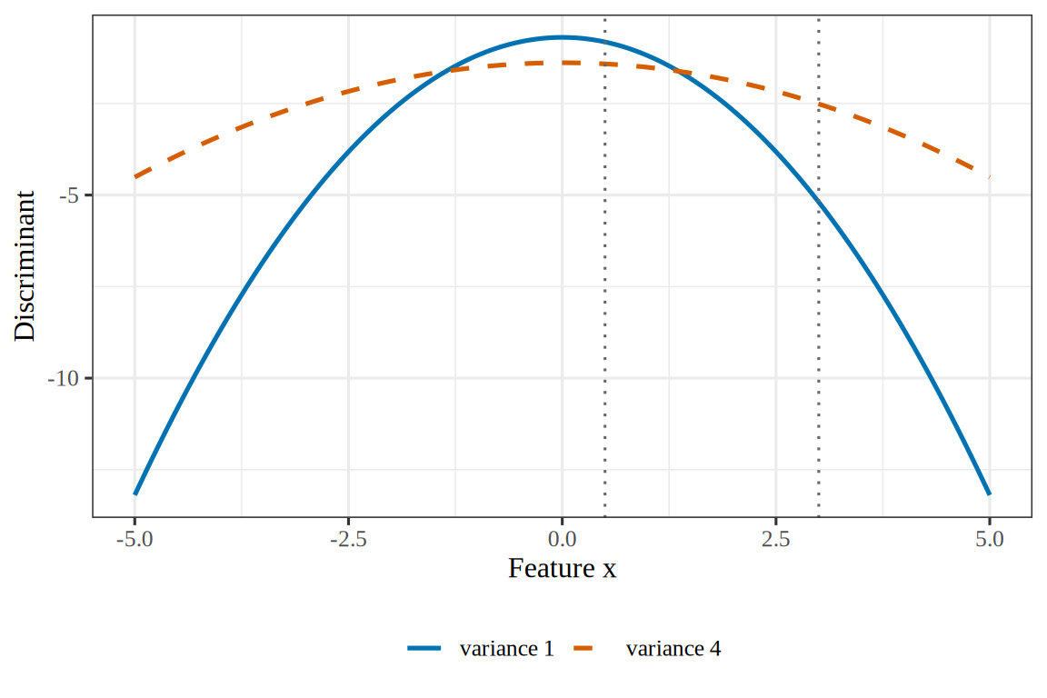
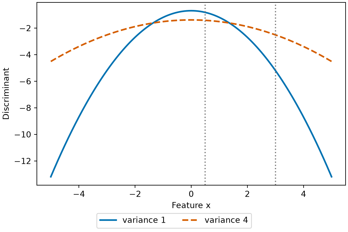
Example 11 (The quadratic discriminant function with one feature) Let \(\ninputvars = 1\), with two classes that have the same mean\(\vm_0 = \vm_1 = 0\), variances\(\Sigma_0 = 1\) and \(\Sigma_1 = 4\), and equal priors. Evaluate the quadratic discriminant function of each class at \(\vx = 0.5\).
ExmExample 12 (The quadratic discriminant with one feature)
Example 12 (The quadratic discriminant with one feature) Let \(\ninputvars = 1\), with two classes that have the same mean\(\vm_0 = 0\) and \(\vm_1 = 0\), variances\(\Sigma_0 = 1\) and \(\Sigma_1 = 4\), and equal priors. Classify \(\vx = 0.5\) and \(\vx = 3\).
By Theorem 4 the discriminants and the densities give the same classes: class 0 for \(\vx = 0.5\) and class 1 for \(\vx = 3\). The narrower class has the larger discriminant near the shared mean, and the wider class has the larger discriminant far from it. So \(\delta_0 = \delta_1\) at two points, \(x = \pm\) 1.36, the roots of a quadratic equation in \(x\). The rule assigns class 0 to the interval between the roots and class 1 to both tails. No linear discriminant can give this rule: with one feature, an affine discriminant difference changes sign at most once, so it splits the line into two pieces, not three.
Figure 7: The two quadratic discriminant functions of Example 12, whose classes have the same mean. The point \(x = 0.5\) (dotted vertical) is between the two crossings, where the class of variance 1 has the higher discriminant, and the point \(x = 3\) is outside them, where the class of variance 4 does, so the two points go to different classes.
CorCorollary 1 (Quadratic discriminant boundaries are quadric surfaces)
Corollary 1 (Quadratic discriminant boundaries are quadric surfaces) Under the assumptions of Theorem 4, let \(k\) and \(l\) be two classes with \(\Sigma_k \ne \Sigma_l\). Then the set on which their quadratic discriminant functions agree,
ExmExample 13 (A circular quadratic discriminant boundary)
Example 13 (A circular quadratic discriminant boundary) Let \(\ninputvars = 2\), with two classes that have the same mean\(\vm_0 = \vm_1 = \vzero\) and the same prior\(\pi_0 = \pi_1 = \frac12\). Their covariance matrices are \(\Sigma_0 = \diag(1, 1)\) and \(\Sigma_1 = \diag(4, 4)\). Then \(\abs{\Sigma_0} = 1\) and \(\abs{\Sigma_1} = 16\), so the quadratic discriminant functions are
So \(\delta_0(\vx) = \delta_1(\vx)\) where \(\frac38 \normsq{\vx} - \frac12 \log 16 = 0\), which is the circle\(\normsq{\vx} =\) 3.7 around the origin. By Corollary 1 this circle is a quadric surface, with \(\matr{A} = \frac38 \diag(1, 1)\), \(\va = \vzero\), and \(c = -\frac12 \log 16\).
Definition 7 (Quadratic discriminant analysis (QDA))Quadratic discriminant analysis is the generative classifier with a multivariate normal density in each class and a separate covariance matrix\(\Sigma_k\) for each class [10]. It predicts the class with the largest quadratic discriminant function of Theorem 4, with each parameter replaced by its estimate. The priors and means are estimated as in Definition 4. Each \(\hSigma_k\) is the sample covariance matrix of the training points in class \(k\) alone, with divisor \(n_k - 1\). R’s MASS::qda() uses that divisor. scikit-learn’s QuadraticDiscriminantAnalysis uses it in version 1.8.0, and it divides by \(n_k\) in version 1.9.1.
The LDA model is the QDA model with the constraint that \(\Sigma_k = \Sigma\) for every class \(k\).
ExmExample 14 (The quadratic boundary for one predictor)
Example 14 (The quadratic boundary for one predictor) Give the two directions of the Smarket days before 2005 their own variances, as in Example 3, and find where the Up and Down discriminant functions of QDA are equal. Setting \(\delta_{\text{Up}}(x) = \delta_{\text{Down}}(x)\) and collecting terms gives a quadratic equation in \(x\).
def delta_qda_py(x, k):return (-np.log(sd_py[k]) - (x - mean_py[k]) **2/ (2* sd_py[k] **2)+ np.log(prior_py[k]))# delta_Up - delta_Down is quadratic in x; fit its three coefficients exactlygrid_py = np.array([-1.0, 0.0, 1.0])coef_py = np.polyfit(grid_py, delta_qda_py(grid_py, "Up") - delta_qda_py(grid_py, "Down"), 2)roots_py = np.sort(np.roots(coef_py))print("roots:", roots_py.round(3))
roots: [ 0.539 23.441]
for x in [-1.0, 1.0, 30.0]: up = delta_qda_py(x, "Up") > delta_qda_py(x, "Down")print(x, "->", "Up"if up else"Down")
-1.0 -> Up
1.0 -> Down
30.0 -> Up
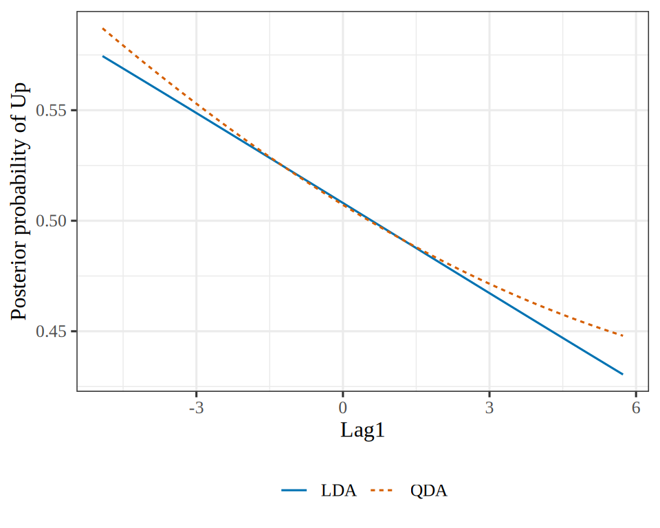
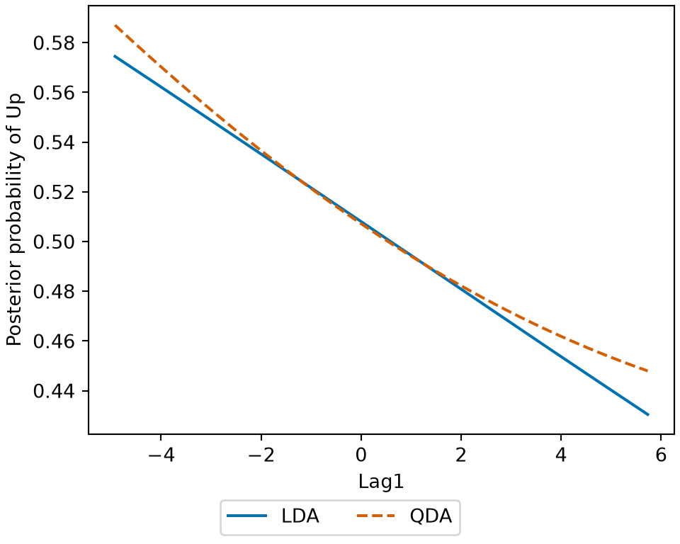
The two discriminant functions are equal at \(x =\) 0.54 and \(x =\) 23.44. The first root is in the middle of the data, where the returns range from -4.9 to 5.7. The second root is far outside that range, so within the range of the data the boundary is a single point, as for LDA. The boundary is curved only because the Up variance, 1.517, differs slightly from the Down variance, 1.507. With the variances this close, the coefficient of \(x^2\) is small, and QDA gives almost the same classifier as LDA.
Figure 8: The posterior probability of Up given Lag1 under LDA (solid) and QDA (dashed) for the Smarket days before 2005, as in Example 6 and Example 14. The two curves nearly coincide, because the two directions have nearly equal spread.
The chain rule of probability holds for every joint distribution, and it has too many parameters to use as it stands: the last factor, \(\Pr(X_N \mid X_1, \dots, X_{N-1})\), is a separate distribution for every combination of the earlier variables. A modeling assumption cuts that down. Conditional independence says that, once some variable is known, other variables carry no further information about each other.
Definition 8 (The naive Bayes assumption) Let \(Y\) be a class label and \(X_1, \dots, X_{\ninputvars}\) the inputfeatures. The naive Bayes assumption is that the features are conditionally independent given the class [11]: \[
\Pr(X_1, \dots, X_{\ninputvars} \mid Y) = \prod_{j=1}^{\ninputvars} \Pr(X_j \mid Y).
\]
ExmExample 15 (Do free and money appear independently in spam?)
Example 15 (Do free and money appear independently in spam?) In the Spambase data [12], let \(Y\) be the class (spam or not), \(X_1\) be “the email contains the word free”, and \(X_2\) be “the email contains the word money”, as in the chain rule example. Restrict to the spam emails (\(Y = 1\)). Compare the jointprobability\(\Pr(X_1 = 1, X_2 = 1 \mid Y = 1)\) with the value \(\Pr(X_1 = 1 \mid Y = 1)\Pr(X_2 = 1 \mid Y = 1)\) that the naive Bayes assumption would give:
import pandas as pdspambase_nb = pd.read_csv("data/spambase.csv")spam_nb = spambase_nb[spambase_nb["Class"] ==1] # keep only the spam emailsp1_nb = (spam_nb["word_freq_free"] >0).mean()p2_nb = (spam_nb["word_freq_money"] >0).mean()joint_nb = ((spam_nb["word_freq_free"] >0) & (spam_nb["word_freq_money"] >0)).mean()print(joint_nb, p1_nb * p2_nb)
0.2410369553226696 0.20490275387446608
spambase_nb<-readr::read_csv("data/spambase.csv", show_col_types =FALSE)spam_nb<-dplyr::filter(spambase_nb, Class==1)# keep only the spam emailsp1_nb<-mean(spam_nb$word_freq_free>0)p2_nb<-mean(spam_nb$word_freq_money>0)joint_nb<-mean(spam_nb$word_freq_free>0&spam_nb$word_freq_money>0)c(joint =joint_nb, product =p1_nb*p2_nb)
    joint   product
0.2410370 0.2049028
Among spam, 54.6% of emails contain free and 37.6% contain money, so under the assumption 20.5% would contain both. The data show 24.1%. The assumption is wrong here, since the two words tend to appear together. A naive Bayes classifier uses the product anyway, and it still often classifies well.
The assumption is rarely exactly true, which is why it is called naive. Its value is in how few parameters it needs.
Example 16 (Counting parameters) Suppose the class\(Y\) takes \(K\) values and each of \(\ninputvars\)features is binary.
Without the naive Bayes assumption, \(\Pr(X_1, \dots, X_{\ninputvars} \mid Y = k)\) is an arbitrary distribution over \(2^{\ninputvars}\) possible values of the binary features, for each class \(k\). It needs \(2^{\ninputvars} - 1\) free numbers per class, since the probabilities must sum to one. With the assumption, each \(\Pr(X_j \mid Y = k)\) is a single Bernoulli probability, so each class needs only \(\ninputvars\) numbers.
Show code
# The number of free parameters in the class-conditional distributions# of K classes with D binary features, with and without the assumption.k_classes<-2d_features<-c(5, 20, 30)full<-k_classes*(2^d_features-1)naive<-k_classes*d_featuresdata.frame( D =d_features, full =format(full, scientific =FALSE), naive =naive)
With 20 binary features and 2 classes, the full model has about 2,097,150 parameters, more than most datasets have observations. The naive Bayes model has 40. The number grows exponentially in \(\ninputvars\) without the assumption, and linearly in \(\ninputvars\) with it.
ExmExample 17 (Gaussian naive Bayes is QDA with diagonal covariance matrices)
Example 17 (Gaussian naive Bayes is QDA with diagonal covariance matrices) Consider a Gaussian naive Bayes classifier with \(\ninputvars\)features. Its class-conditional density multiplies \(\ninputvars\)normal densities with means\(\mean_{kj}\) and variances\(\sigma_{kj}^2\). That multiplication gives the multivariate normal density with mean vector \(\vm_k = (\mean_{k1}, \dots, \mean_{k\ninputvars})\) and diagonalcovariance matrix\(\covmat_k = \diagf{\sigma_{k1}^2, \dots, \sigma_{k\ninputvars}^2}\). So the classifier is QDA with each \(\covmat_k\) restricted to be diagonal.
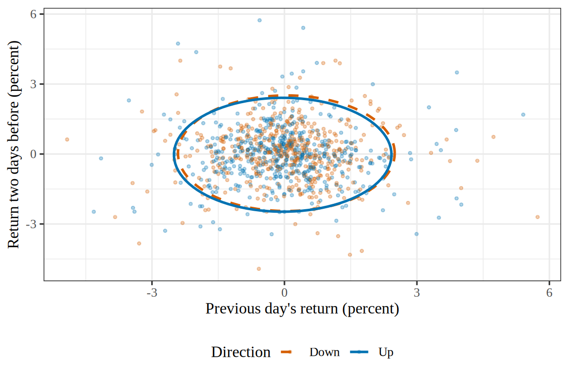
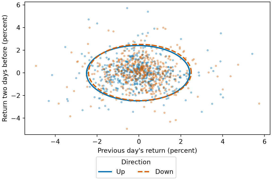
For the Smarket days before 2005, with features Lag1 and Lag2, the ellipses of Figure 9 have axes parallel to the coordinate axes, because each \(\covmat_k\) is diagonal.
Show code
library(dplyr)# nolint: undesirable_function_linterlibrary(ggplot2)# nolint: undesirable_function_linterangle<-seq(0, 2*pi, length.out =100)nbc_angles<-tibble(angle =angle)nbc_class_stats<-da_train|>summarize( .by =Direction, Lag1_mean =mean(Lag1), Lag1_sd =sd(Lag1), Lag2_mean =mean(Lag2), Lag2_sd =sd(Lag2))nbc_ellipses<-nbc_class_stats|>cross_join(nbc_angles)|>mutate( Lag1 =Lag1_mean+2*Lag1_sd*cos(angle), Lag2 =Lag2_mean+2*Lag2_sd*sin(angle))nbc_colours<-c(Up ="#0072B2", Down ="#D55E00")nbc_linetypes<-c(Up ="solid", Down ="dashed")da_train|>ggplot()+aes(Lag1, Lag2, colour =Direction, linetype =Direction)+geom_point(alpha =0.3, size =0.8)+geom_path(data =nbc_ellipses, linewidth =0.9)+scale_colour_manual(values =nbc_colours)+scale_linetype_manual(values =nbc_linetypes)+labs( x ="Previous day's return (percent)", y ="Return two days before (percent)")
Definition 11 (K-nearest neighbors classifier) For a positive integer\(K\) of neighbors and a feature vector\(\vx\), the K-nearest neighbors classifier finds the \(K\)training points closest to \(\vx\) in Euclidean distance, and predicts the most frequent class among them [5, Sec. 4.7.6]. The K-nearest neighbors classifier estimates\(\Pr(\Outvar = k \mid \vX = \vx)\) by the fraction of those \(K\) points in class \(k\), so K-nearest neighbors makes no assumption about the form of \(f_k\). The nonparametric models chapter studies K-nearest neighbors further.
ExmExample 18 (The nearest neighbors of one Smarket day)
Example 18 (The nearest neighbors of one Smarket day) Consider a day on which Lag1 was \(0.5\) and Lag2 was \(-0.5\). For \(K = 5\), the five Smarkettraining days closest to that point in Euclidean distance are the neighbors the K-nearest neighbors classifier counts.
Of the five neighbors, 2 were up days and 3 were down days, so the classifierestimates\(\Pr(\Outvar = \text{Up} \mid \vX = \vx)\) as 0.4 and predicts Down.
Exercise 19 (Counting parameters) Consider a classification problem with \(K\) classes and \(\ninputvars\)features. A symmetric\(\ninputvars \times \ninputvars\) matrix has \(\ninputvars(\ninputvars+1)/2\) free entries. Count the free parameters of LDA (Definition 4).
Solution 19. LDA has \(K - 1\) free priors, because the priors sum to one, and \(K\ninputvars\) entries in the \(K\)classmeans. Its one covariance matrix is symmetric, so it adds \(\ninputvars(\ninputvars+1)/2\) free entries. The total is \((K - 1) + K\ninputvars + \ninputvars(\ninputvars+1)/2\)parameters.
Solution 20. QDA has the same \(K - 1\) priors and \(K\ninputvars\)mean entries as LDA, and \(K\)covariance matrices instead of one: \((K - 1) + K\ninputvars + K\,\ninputvars(\ninputvars+1)/2\)parameters.
Solution 23. As \(\ninputvars\) grows, the LDA count grows like \(\ninputvars^2/2\), and the QDA count like \(K \ninputvars^2/2\). The naive Bayes and logistic counts grow only linearly in \(\ninputvars\). Each QDA covariance matrix is estimated from only the \(n_k\) points of its own class, so when the classes are small, QDA’s estimates vary more from one training set to another than those of any of the other models.
LemTheorem 5 (Parameter counts of the classifiers)
Theorem 5 (Parameter counts of the classifiers) With \(K\) classes and \(\ninputvars\)features, the number of free parameters is
Table 1: The number of free parameters of each method.
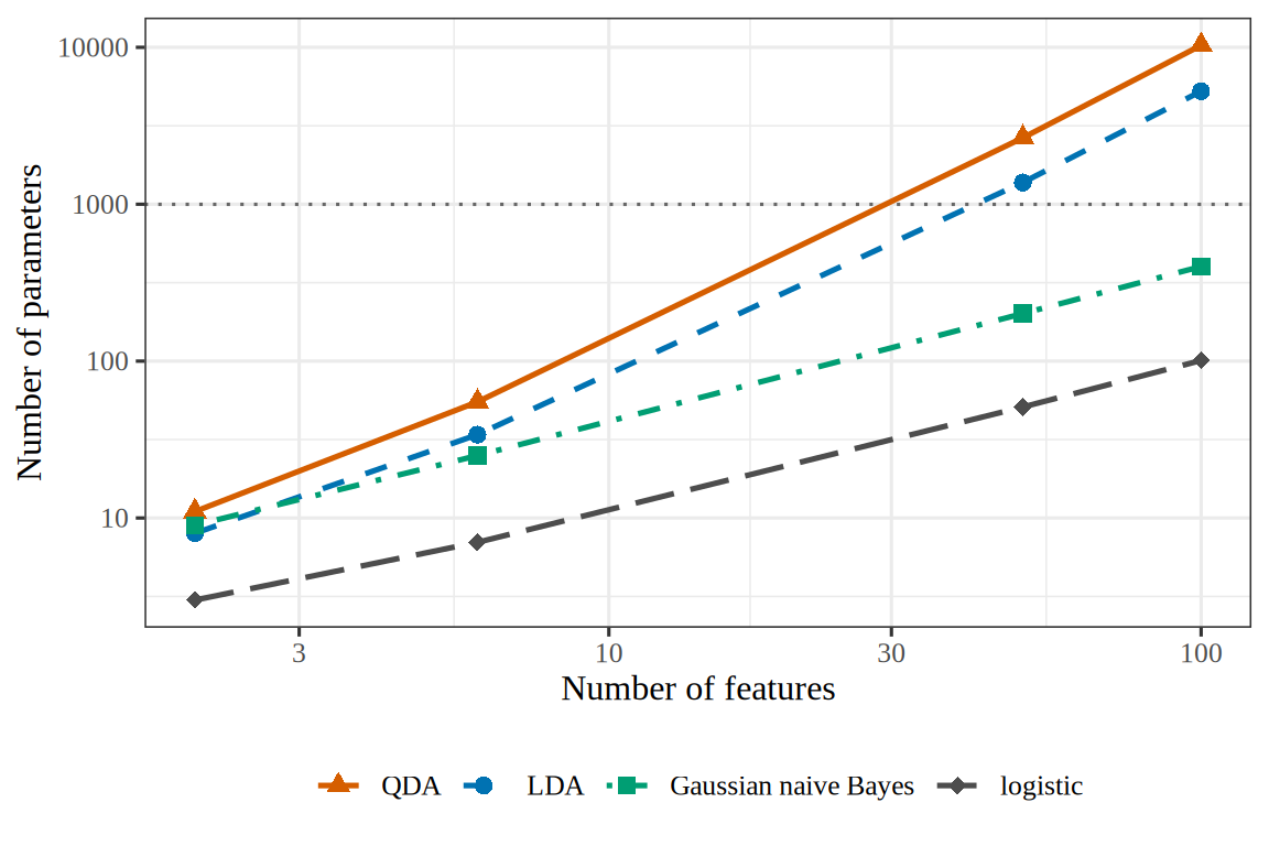
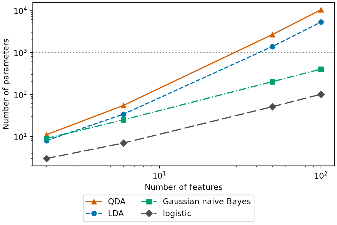
Example 19 (Parameters for two classes) Count the parameters of Theorem 5 for \(K = 2\)classes and several numbers of features\(\ninputvars\), including \(\ninputvars = 2\), for two lagged returns, and the \(\ninputvars = 6\) of the Smarket fit exercise.
At \(\ninputvars =\) 50 the QDA model has 2,651 parameters and LDA has 1,376, against 51 for logistic regression. The Smarkettraining set has 998 days, which is 0.38 observations per QDAparameter at \(\ninputvars =\) 50. At \(\ninputvars =\) 100 QDA has 10,301 parameters, more than the 998 training days.
Figure 10: The parameter counts of Example 19 for two classes, with the number of Smarket training days (dotted line). The quadratic model has more parameters than there are training days somewhere between 6 and 50 features.
The pooled covariance matrix of LDA is invertible, since it has 58 degrees of freedom of within-class variation, more than \(40\), but it estimates 820 free entries from them, so its estimate is noisy.
The diagonalcovariance matrices of naive Bayes have only \(\ninputvars\)variances per class, so their estimates are the most stable of the three.
ExrExercise 25 (Choosing among the classifiers (part 2))
Exercise 25 (Choosing among the classifiers (part 2)) Use the setup of Exercise 24.
There are \(\nobs = 100{,}000\) observations and \(\ninputvars = 3\)features, and a plot shows that the within-class spread of the features differs a lot between classes.
Solution 25. QDA. With \(3\)features and two classes, QDA has 19 parameters and LDA 13, by Theorem 5, and they are estimated from \(100{,}000\) points. The unequal spreads are structure that LDA’s single covariance matrix cannot represent, so LDA is biased here, and QDA can represent it.
ExrExercise 26 (Choosing among the classifiers (part 3))
Exercise 26 (Choosing among the classifiers (part 3)) Use the setup of Exercise 24.
Some features are binary indicators, such as whether a word appears in an email.
Solution 27. Moving from LDA to QDA adds parameters. That lowers the bias when the classes really differ in their covariance matrices, and it raises the variance of the estimates, because each classcovariance matrix is estimated from that class alone. LDA accepts bias from forcing one covariance matrix on all classes, in exchange for estimating only one matrix, from all \(\nobs\) points. Gaussian naive Bayes restricts each class covariance matrix to be diagonal instead, so it has the fewest parameters of the three generative models when \(\ninputvars\) is large, and it is biased when the features are correlated within a class. QDA is the better choice when \(\nobs\) is large relative to its number of parameters in Theorem 5, and LDA when \(\nobs\) is small [2, Ch. 4]. Regularized discriminant analysis compromises between the two by shrinking each \(\hSigma_k\) toward the pooled \(\hSigma\)[8, Sec. 4.3.1].
6 Lab: discriminant analysis, naive Bayes and nearest neighbors on the stock market data
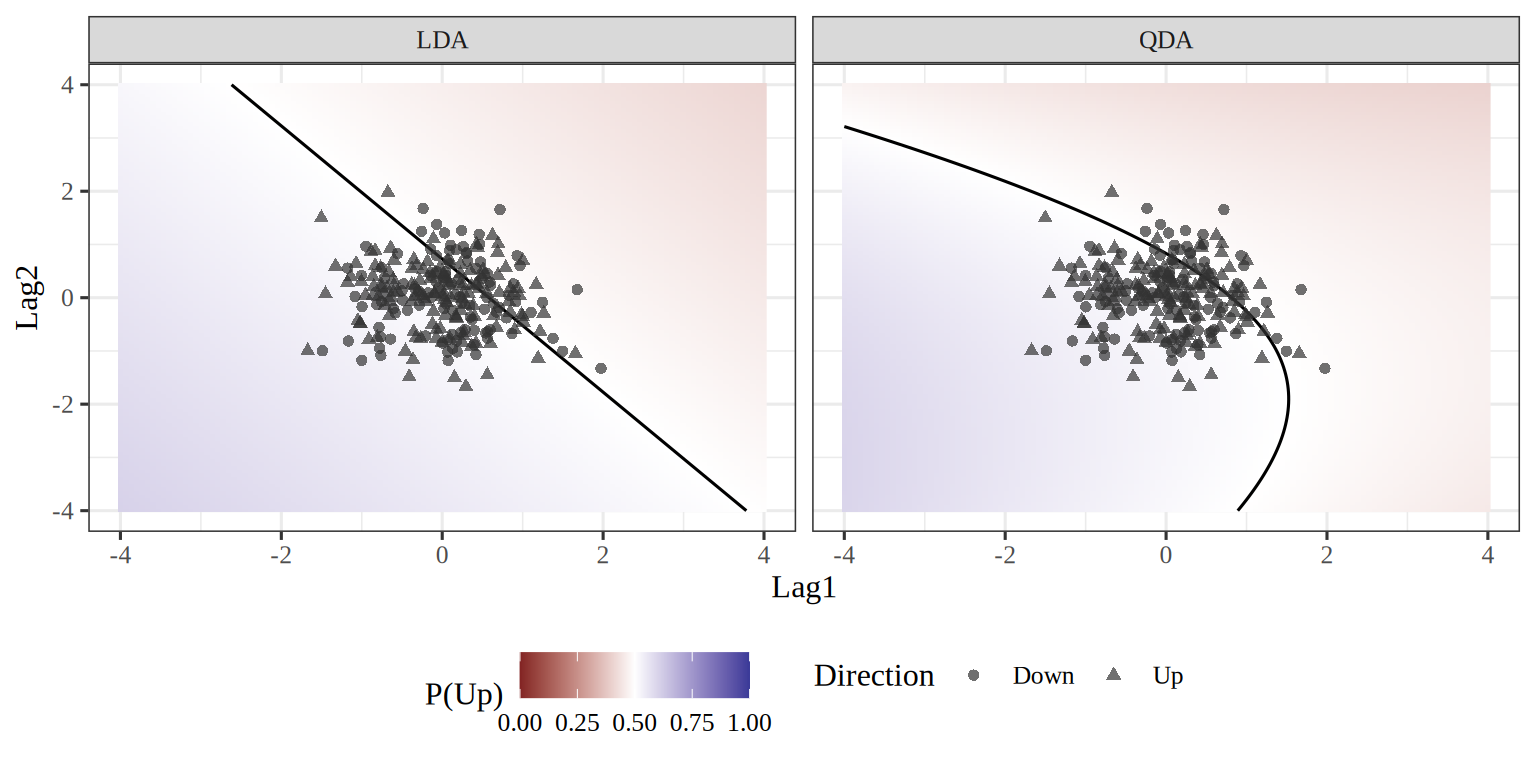
Exercise 28 (LDA and QDA on the stock market) Use the Smarket days of the Smarket fit exercise. Fit LDA and QDA for the direction of the market with Lag1 and Lag2 as the only predictors, on the days before 2005. Predict each day of 2005 and tabulate the predictions against what happened.
What are the fitted class proportions and class means?
da_test<-da[da$Year==2005, ]lda2<-MASS::lda(Direction~Lag1+Lag2, data =da_train)qda2<-MASS::qda(Direction~Lag1+Lag2, data =da_train)# The six-predictor logistic regression of the Smarket fit exercise, scored on the same days.glm_fit<-glm(I(Direction=="Up")~Lag1+Lag2+Lag3+Lag4+Lag5+Volume, data =da_train, family =binomial)pred_glm<-ifelse(predict(glm_fit, da_test, type ="response")>0.5, "Up", "Down")acc_glm<-mean(pred_glm==da_test$Direction)lda2$prior
    Down       Up
0.491984 0.508016
lda2$means
            Lag1        Lag2
Down  0.04279022  0.03389409
Up   -0.03954635 -0.03132544
pred_lda<-predict(lda2, da_test)$classpred_qda<-predict(qda2, da_test)$classtable(LDA =pred_lda, actual =da_test$Direction)
# 95% intervals for each accuracy, and for the paired differences between rules# scored on the same days, as for the logistic regression of the Smarket fit exercise.wald_ci<-function(p, n){p+c(lower =-1, upper =1)*qnorm(0.975)*sqrt(p*(1-p)/n)}paired_ci<-function(a, b){d<-as.integer(a)-as.integer(b)mean(d)+c(lower =-1, upper =1)*qt(0.975, length(d)-1)*sd(d)/sqrt(length(d))}ci_acc<-sapply(acc, wald_ci, n =nrow(da_test))hit_lda<-pred_lda==da_test$Directionhit_qda<-pred_qda==da_test$Directionhit_up<-da_test$Direction=="Up"ci_qda_up<-paired_ci(hit_qda, hit_up)ci_qda_lda<-paired_ci(hit_qda, hit_lda)
for name, model in [("LDA", lda2_py), ("QDA", qda2_py)]: pred = model.predict(da_test_py[features_py]) acc_py =float((pred == da_test_py["Direction"]).mean())# A 95% interval for the accuracy: the proportion plus or minus 1.96 standard errors. half_py =1.96* np.sqrt(acc_py * (1- acc_py) /len(da_test_py))print(name, "accuracy:", round(acc_py, 3), [round(float(acc_py - half_py), 3), round(float(acc_py + half_py), 3)])print(pd.crosstab(pred, da_test_py["Direction"], rownames=["predicted"], colnames=["actual"]))
LDA accuracy: 0.56 [0.498, 0.621]
actual     Down   Up
predicted
Down         35   35
Up           76  106
QDA accuracy: 0.599 [0.539, 0.66]
actual     Down   Up
predicted
Down         30   20
Up           81  121
The classes are balanced, with 50.8% of the training days up. The means of both lags are slightly negative on days that went up and slightly positive on days that went down: -0.040 and 0.043 for Lag1, and -0.031 and 0.034 for Lag2. The gap between the Lag1 means, 0.08, is small next to the standard deviation of Lag1 within a class, about 1.23, so the classes overlap almost completely.
ExrExercise 29 (LDA and QDA on the stock market (part 2))
Exercise 29 (LDA and QDA on the stock market (part 2)) Use the setup of Exercise 28.
Solution 29. LDA is right on 56% of the 252 days in 2005 (95% interval [49.8, 62.1]%), QDA on 59.9% ([53.9, 66]%), and always predicting Up on 56% ([49.8, 62.1]%). LDA does no better than the constant rule that always predicts Up, and the logistic regression of its solution, with more predictors, was right on only 48%. QDA exceeds the accuracy of the constant rule by 4 percentage points.
ExrExercise 30 (LDA and QDA on the stock market (part 3))
Exercise 30 (LDA and QDA on the stock market (part 3)) Use the setup of Exercise 28.
How much trust does the accuracy difference between the two models deserve, given that it comes from one year of data?
The rules are scored on the same days, so the sharper comparison is day by day. QDA exceeds the accuracy of the constant rule by 4 percentage points (95% interval [-1.5, 9.5]), an interval that includes 0. It exceeds the accuracy of LDA by 4 percentage points ([0.5, 7.4]), an interval that excludes 0.
These intervals reflect sampling variation across the test days in 2005, not across training sets, and they do not account for comparing several rules on the same days before reporting the best. Showing that QDA has higher out-of-sample accuracy would need more test days or repeated splits.
Figure 11: Predicted probability of an up day from the LDA and QDA fits of Solution 28, over the plane of the two lagged returns. The black line and curve are the decision boundaries, where the probability is one half. The points are the days of 2005.
Figure 12: The graph of the predicted probability of an up day of Figure 11, as a surface over the plane of the two lagged returns. The gray plane is at probability one half, and the decision boundary is where it cuts the surface: a line for LDA and a curve for QDA.
Show code
sm_axis<-seq(-4, 4, length.out =60)sm_grid<-tidyr::expand_grid(Lag1 =sm_axis, Lag2 =sm_axis)sm_n<-length(sm_axis)sm_lda_fit<-predict(lda2, sm_grid)sm_qda_fit<-predict(qda2, sm_grid)sm_lda_z<-matrix(sm_lda_fit$posterior[, "Up"], nrow =sm_n)sm_qda_z<-matrix(sm_qda_fit$posterior[, "Up"], nrow =sm_n)sm_half<-matrix(0.5, nrow =sm_n, ncol =sm_n)sm_stops<-c(0, 0.5, 1)sm_cols<-c("#0072B2", "#F2F2F2", "#D55E00")sm_scale<-list(sm_stops, sm_cols)sm_grey<-c("#808080", "#808080")sm_plane_stops<-c(0, 1)sm_plane_scale<-list(sm_plane_stops, sm_grey)sm_eye<-list(x =1.6, y =-1.6, z =0.9)sm_camera<-list(eye =sm_eye)sm_xaxis<-list(title ="Lag1")sm_yaxis<-list(title ="Lag2")sm_zrange<-c(0, 1)sm_zaxis<-list(title ="P(Up)", range =sm_zrange)sm_scene<-list( xaxis =sm_xaxis, yaxis =sm_yaxis, zaxis =sm_zaxis, camera =sm_camera)sm_lda_plot<-plotly::plot_ly()|>plotly::add_surface( x =sm_axis, y =sm_axis, z =sm_lda_z, cmin =0, cmax =1, colorscale =sm_scale, showscale =FALSE)|>plotly::add_surface( x =sm_axis, y =sm_axis, z =sm_half, colorscale =sm_plane_scale, showscale =FALSE, opacity =0.3, hoverinfo ="skip")|>plotly::layout(scene =sm_scene)sm_lda_plot
sm_qda_plot<-plotly::plot_ly()|>plotly::add_surface( x =sm_axis, y =sm_axis, z =sm_qda_z, cmin =0, cmax =1, colorscale =sm_scale, showscale =FALSE)|>plotly::add_surface( x =sm_axis, y =sm_axis, z =sm_half, colorscale =sm_plane_scale, showscale =FALSE, opacity =0.3, hoverinfo ="skip")|>plotly::layout(scene =sm_scene)sm_qda_plot
Show code
import htmlfig_alt = r.qda_alt_sfsm_qda_model = QuadraticDiscriminantAnalysis().fit(sm_x_3d, sm_y_3d)# `classes_` is sorted, so the column of "Up" comes after "Down".sm_qda_up = sm_qda_model.predict_proba(sm_points_3d)[:, 1]sm_qda_z_3d = sm_qda_up.reshape(sm_lag1_3d.shape)fig = go.Figure(data=[ go.Surface( x=sm_axis_3d, y=sm_axis_3d, z=sm_qda_z_3d, colorscale=sm_scale_3d, cmin=0, cmax=1, showscale=False, opacity=0.9, ), go.Surface( x=sm_axis_3d, y=sm_axis_3d, z=np.full_like(sm_qda_z_3d, 0.5), colorscale=[[0, "grey"], [1, "grey"]], showscale=False, opacity=0.3, ),])fig.update_layout( scene=dict( xaxis_title="Lag1", yaxis_title="Lag2", zaxis_title="P(Up)", zaxis=dict(range=[0, 1]), ),);print("```{=html}\n"+f'<div role="group" aria-label="{html.escape(fig_alt)}">\n'+ fig.to_html(full_html=False, include_plotlyjs="cdn")+"\n</div>\n```")
sd_stops<-c(0, 1)sd_blue_cols<-c("#C6DBEF", "#0072B2")sd_orange_cols<-c("#FDE0C5", "#D55E00")sd_blue<-list(sd_stops, sd_blue_cols)sd_orange<-list(sd_stops, sd_orange_cols)sd_eye<-list(x =1.6, y =-1.6, z =0.9)sd_xaxis<-list(title ="Lag1")sd_yaxis<-list(title ="Lag2")sd_zaxis<-list(title ="prior times density")sd_camera<-list(eye =sd_eye)sd_scene<-list( xaxis =sd_xaxis, yaxis =sd_yaxis, zaxis =sd_zaxis, camera =sd_camera)sd_legend<-list(orientation ="h", x =0, y =-0.05)sd_plot<-plotly::plot_ly()|>plotly::add_surface( x =sd_axis, y =sd_axis, z =sd_up_z, name ="Up", showlegend =TRUE, colorscale =sd_blue, showscale =FALSE, opacity =0.8)|>plotly::add_surface( x =sd_axis, y =sd_axis, z =sd_down_z, name ="Down", showlegend =TRUE, colorscale =sd_orange, showscale =FALSE, opacity =0.8)|>plotly::layout(scene =sd_scene, legend =sd_legend)sd_plot
ExrExercise 31 (Lab: split the Smarket data by year)
Exercise 31 (Lab: split the Smarket data by year) Split the Smarket data [5] into a training set of the days before \(2005\) and a test set of the days in \(2005\). Keep Lag1 and Lag2 as the predictors and Direction as the outcome.
from sklearn.neighbors import KNeighborsClassifierknn1_py = KNeighborsClassifier(n_neighbors=1).fit(x_train, y_train)knn1_py_error =float((knn1_py.predict(x_test) != y_test).mean())knn1_py_error
0.5
set.seed(1)knn1_pred<-class::knn(x_train, x_test, y_train, k =1)knn1_r_error<-mean(knn1_pred!=y_test)knn1_r_error
[1] 0.5
The test error at \(K = 1\) is 0.50 in the R run and 0.50 in the Python run. Both are near \(0.5\), the error of a coin flip, which suggests that Lag1 and Lag2 carry little information about the direction of the market.
ExrExercise 33 (Lab: find the test error at K = 3)
Exercise 33 (Lab: find the test error at K = 3) Fit a \(K\)-nearest-neighbors classifier with \(K = 3\) to the training set of Solution 31, and find its test error.
The test error is 0.41 in the R run and 0.40 in the Python run.
7 Further reading
ReadingRead
James et al. [2], Chapter 4, derives these classifiers and compares them with logistic regression. Hastie et al. [8], Section 4.3, covers discriminant analysis, including its regularized versions.
B. Hutchinson, “DATA 471/571: Machine learning.” Western Washington University, 2024.
[2]
G. James, D. Witten, T. Hastie, and R. Tibshirani, An introduction to statistical learning with applications in R, 2nd ed. Springer, 2021. Available: https://www.statlearning.com/
G. James, D. Witten, T. Hastie, R. Tibshirani, and J. Taylor, An introduction to statistical learning: With applications in Python. Springer, 2023. doi: 10.1007/978-3-031-38747-0.
W. N. Venables and B. D. Ripley, Modern applied statistics with S, 4th ed. in Statistics and computing. Springer, 2002. doi: 10.1007/978-0-387-21706-2.
[8]
T. Hastie, R. Tibshirani, and J. Friedman, The elements of statistical learning: Data mining, inference, and prediction, 2nd ed. Springer, 2009. Available: https://hastie.su.domains/ElemStatLearn/