Measures and Probability Measures

0.1 Measures

DefDefinition 1 (Measure)

Definition 1 (Measure) A measure on a set \(S\) [1] with a \(\sigma\)-algebra \(\mathcal{S}\) is a function \(\mu: \mathcal{S}\to [0, \infty]\) that satisfies:

• \(\mu(\emptyset) = 0\).
• \(\mu\) is countably additive.

ExmExample 1 (Counting elements is a measure)

Example 1 (Counting elements is a measure) The counting function \(\mu(A) \stackrel{\text{def}}{=}\mathopen{}\left|A\right|\mathclose{}\) of Example 1 in Additivity, defined on the \(\sigma\)-algebra of all subsets of \(D\) (Example 1 in Sigma-Algebras), takes values in \([0, \infty]\), is countably additive (Example 3 in Additivity), and gives \(\mu(\emptyset) = 0\), so it is a measure.

CorCorollary 1 (Measures are finitely additive)

Corollary 1 (Measures are finitely additive) Every measure is finitely additive.

ProofProof

Proof. A measure \(\mu\) is countably additive and has \(\mu(\emptyset) = 0\) (Definition 1), so Theorem 1 in Additivity applies to it.

DefDefinition 2 (Counting measure)

Definition 2 (Counting measure) The counting measure [2] on a set \(S\) is the measure on the \(\sigma\)-algebra of all subsets of \(S\) that assigns each finite set its number of elements, and each infinite set the value \(\infty\):

\[ \mu(A) \stackrel{\text{def}}{=}\begin{cases} \mathopen{}\left|A\right|\mathclose{} & \text{if } A \text{ is finite} \\ \infty & \text{if } A \text{ is infinite} \end{cases} \]

ExmExample 2 (Counting measure on the non-negative integers)

Example 2 (Counting measure on the non-negative integers) For the counting measure \(\mu\) on the non-negative integers \({\mathopen{}\left\{0, 1, 2, \ldots\right\}\mathclose{}}\), \(\mu({\mathopen{}\left\{0, 1, 2\right\}\mathclose{}}) = 3\), and the set of even numbers has \(\mu({\mathopen{}\left\{0, 2, 4, \ldots\right\}\mathclose{}}) = \infty\). The even numbers are the union of the pairwise disjoint sets \({\mathopen{}\left\{0\right\}\mathclose{}}, {\mathopen{}\left\{2\right\}\mathclose{}}, {\mathopen{}\left\{4\right\}\mathclose{}}, \ldots\), and countable additivity agrees:

\[ \begin{aligned} \sum_{k=0}^{\infty} \mu({\mathopen{}\left\{2k\right\}\mathclose{}}) &= 1 + 1 + \cdots \\ &= \infty. \end{aligned} \]

DefDefinition 3 (Measurable space)

Definition 3 (Measurable space) A measurable space [3] \((S, \mathcal{S})\) is a set \(S\) together with a \(\sigma\)-algebra \(\mathcal{S}\) on \(S\).

DefDefinition 4 (Measurable set)

Definition 4 (Measurable set) In a measurable space \((S, \mathcal{S})\), the sets in \(\mathcal{S}\) are its measurable sets.

ExmExample 3 (Measurable spaces of die rolls)

Example 3 (Measurable spaces of die rolls) For the die rolls \(D = {\mathopen{}\left\{1, 2, 3, 4, 5, 6\right\}\mathclose{}}\):

• \((D, \mathcal{S})\), with \(\mathcal{S}\) the collection of all subsets of \(D\), is a measurable space (Example 1 in Sigma-Algebras).
• \((D, {\mathopen{}\left\{\emptyset, {\mathopen{}\left\{2, 4, 6\right\}\mathclose{}}, {\mathopen{}\left\{1, 3, 5\right\}\mathclose{}}, D\right\}\mathclose{}})\) is also a measurable space. Its measurable sets are only those four; for example, \({\mathopen{}\left\{1\right\}\mathclose{}}\) is not one of them.

DefDefinition 5 (Measure space)

Definition 5 (Measure space) A measure space \((S, \mathcal{S}, \mu)\) is a measurable space together with a measure \(\mu\) on \(\mathcal{S}\).

ExmExample 4 (Measure space of die rolls)

Example 4 (Measure space of die rolls) For the die rolls \(D = {\mathopen{}\left\{1, 2, 3, 4, 5, 6\right\}\mathclose{}}\), adding the counting function \(\mu(A) = \mathopen{}\left|A\right|\mathclose{}\) of Example 1 to the measurable space \((D, \mathcal{S})\) of Example 3 makes \((D, \mathcal{S}, \mu)\) a measure space.

DefDefinition 6 (Lebesgue measure)

Definition 6 (Lebesgue measure) Lebesgue measure on \(\mathbb{R}\) [4] is the measure \(\lambda\) on the Borel \(\sigma\)-algebra \(\mathcal{B}\) that assigns each interval its length: for real numbers \(a \le b\),

\[ \begin{aligned} \lambda([a, b]) &= \lambda((a, b)) \\ &= \lambda([a, b)) \\ &= \lambda((a, b]) \\ &\stackrel{\text{def}}{=}b - a, \end{aligned} \]

and \(\lambda(I) \stackrel{\text{def}}{=}\infty\) for each unbounded interval \(I\).

RemarkRemark 1 (Lebesgue measure exists)

Remark 1 (Lebesgue measure exists). Exactly one measure on \(\mathcal{B}\) assigns every interval its length; constructing it takes more measure theory than these notes cover [4], which also extends \(\lambda\) to a larger \(\sigma\)-algebra, the Lebesgue-measurable sets, with the same values on Borel sets.

DefDefinition 7 (Lebesgue measure on an interval)

Definition 7 (Lebesgue measure on an interval) Lebesgue measure on an interval \(I\), such as \([0, 1]\), is \(\lambda\) (Definition 6) applied only to the Borel sets that are subsets of \(I\).

ExmExample 5 (Lengths of some Borel sets)

Example 5 (Lengths of some Borel sets)  

• \[ \begin{aligned} \lambda([2, 5]) &= 5 - 2 \\ &= 3. \end{aligned} \]

• A single point has length zero:

  \[ \begin{aligned} \lambda({\mathopen{}\left\{a\right\}\mathclose{}}) &= \lambda([a, a]) \\ &= a - a \\ &= 0. \end{aligned} \]

• The integers are the union of the pairwise disjoint single points \({\mathopen{}\left\{0\right\}\mathclose{}}, {\mathopen{}\left\{1\right\}\mathclose{}}, {\mathopen{}\left\{-1\right\}\mathclose{}}, {\mathopen{}\left\{2\right\}\mathclose{}}, {\mathopen{}\left\{-2\right\}\mathclose{}}, \ldots\) (Example 6 in Sigma-Algebras), so countable additivity gives

  \[ \begin{aligned} \lambda(\mathbb{Z}) &= 0 + 0 + \cdots \\ &= 0. \end{aligned} \]

• \(\lambda([0, \infty)) = \infty\), because \([0, \infty)\) is unbounded.

• Lebesgue measure on \([0, 1]\) gives the whole interval \([0, 1]\) the value

  \[ \begin{aligned} \lambda([0, 1]) &= 1 - 0 \\ &= 1. \end{aligned} \]

RemarkRemark 2 (Measures generalize size)

Remark 2 (Measures generalize size). A measure generalizes size: it can measure how many elements a set has, as in Definition 2, or how long a set of real numbers is, as Lebesgue measure (Definition 6) does, assigning each interval \([a, b]\) its length \(b - a\). For example, the counting measure on \({\mathopen{}\left\{0, 1, 2, \ldots\right\}\mathclose{}}\) gives \({\mathopen{}\left\{2, 3, 4, 5\right\}\mathclose{}}\) the value \(4\), while the Lebesgue measure of the interval \([2, 5]\) is \(5 - 2 = 3\). Both can serve as the measures \(\mu_1\) and \(\mu_2\) in the Tonelli and Fubini theorems.

DefDefinition 8 (Measure zero, null set)

Definition 8 (Measure zero, null set) Let \((S, \mathcal{S}, \mu)\) be a measure space. A set \(A \in \mathcal{S}\) has measure zero [5] (also called a null set for \(\mu\)) if \(\mu(A) = 0\).

ExmExample 6 (Sets of measure zero)

Example 6 (Sets of measure zero)  

• For a counting measure, only \(\emptyset\) has measure zero: a nonempty set has at least one element, so its counting measure is at least \(1\).
• For Lebesgue measure, every single point \({\mathopen{}\left\{a\right\}\mathclose{}}\) and the integers \(\mathbb{Z}\) have measure zero (Example 5), although neither set is empty.

DefDefinition 9 (Almost everywhere (\(\mu\)-almost everywhere, \(\mu\)-a.e.))

Definition 9 (Almost everywhere (\(\mu\)-almost everywhere, \(\mu\)-a.e.)) Let \((S, \mathcal{S}, \mu)\) be a measure space. A statement about the elements of \(S\) holds \(\mu\)-almost everywhere (written \(\mu\)-a.e., or almost everywhere when \(\mu\) is clear from context) [6] if the set of elements for which it fails is a subset of a set of measure zero.

ExmExample 7 (Non-negative except on the integers)

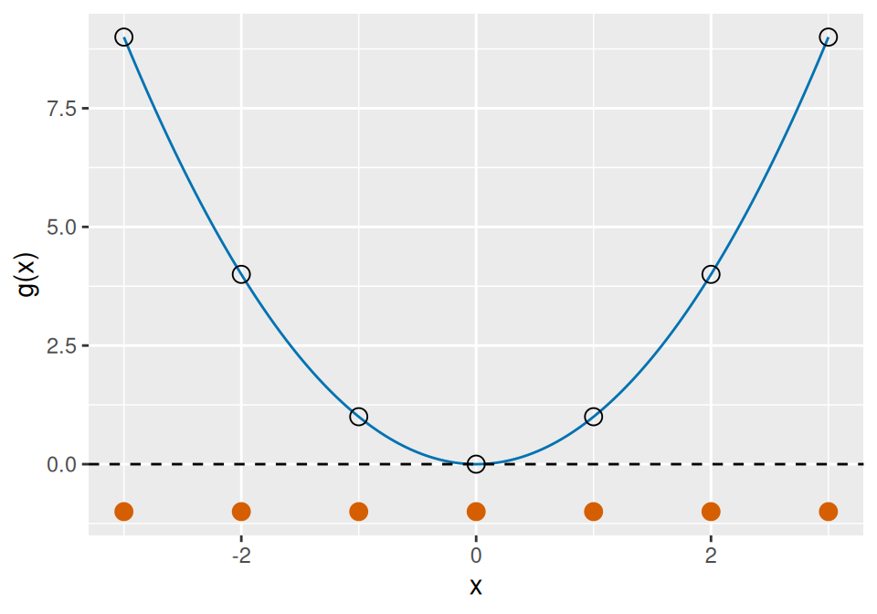
Example 7 (Non-negative except on the integers) Let \(g : \mathbb{R}\to \mathbb{R}\) with \(g(x) = -1\) when \(x\) is an integer and \(g(x) = x^2\) otherwise. The statement “\(g(x) \ge 0\)” fails exactly for \(x \in \mathbb{Z}\), and \(\lambda(\mathbb{Z}) = 0\) (Example 5), so \(g \ge 0\) holds \(\lambda\)-almost everywhere, though not everywhere.

For a counting measure, only \(\emptyset\) has measure zero (Example 6), so a statement holds almost everywhere only if it holds everywhere.

aeg_x_pf <- seq(-3, 3, length.out = 301)
aeg_curve_pf <- tibble::tibble(x = aeg_x_pf, y = aeg_x_pf^2)
aeg_ints_pf <- -3:3
aeg_open_pf <- tibble::tibble(x = aeg_ints_pf, y = aeg_ints_pf^2)
aeg_dots_pf <- tibble::tibble(x = aeg_ints_pf, y = -1)
aeg_aes_pf <- ggplot2::aes(x, y)
ggplot2::ggplot(aeg_curve_pf, aeg_aes_pf) +
  ggplot2::geom_line(colour = "#0072B2") +
  ggplot2::geom_point(data = aeg_open_pf, shape = 1, size = 3) +
  ggplot2::geom_point(data = aeg_dots_pf, colour = "#D55E00", size = 3) +
  ggplot2::geom_hline(yintercept = 0, linetype = "dashed") +
  ggplot2::labs(x = "x", y = "g(x)")

import matplotlib.pyplot as plt
import numpy as np

aeg_x_pf = np.linspace(-3, 3, 301)
aeg_ints_pf = np.arange(-3, 4)
fig, ax = plt.subplots(figsize=(5, 3.5), layout="constrained")
ax.plot(aeg_x_pf, aeg_x_pf**2, color="#0072B2")
ax.plot(aeg_ints_pf, aeg_ints_pf**2, linestyle="", marker="o",
        markerfacecolor="white", color="black")
ax.plot(aeg_ints_pf, -np.ones(7), linestyle="", marker="o", color="#D55E00")
ax.axhline(0, linestyle="dashed", color="black")
ax.set_xlabel("x")
ax.set_ylabel("g(x)")
plt.show()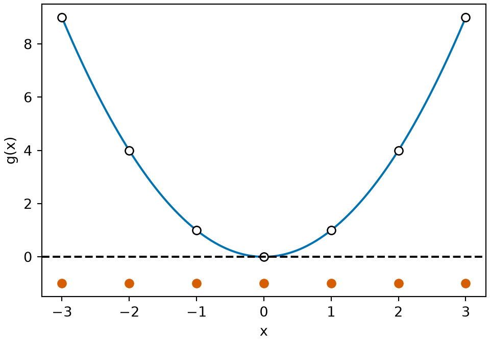

Figure 1: The plot shows the function \(g\) of Example 7 on \([-3, 3]\). It is \(x^2\) except at the integers, where it is \(-1\). It falls below the dashed line \(g = 0\) only at those points, which together have measure zero, so \(g \ge 0\) almost everywhere.

R

Python

DefDefinition 10 (Finite measure)

Definition 10 (Finite measure) Let \((S, \mathcal{S}, \mu)\) be a measure space. The measure \(\mu\) is finite if [7] \(\mu(S) < \infty\).

DefDefinition 11 (\(\sigma\)-finite measure)

Definition 11 (\(\sigma\)-finite measure) Let \((S, \mathcal{S}, \mu)\) be a measure space. The measure \(\mu\) is \(\sigma\)-finite [8] if \(S\) is the union \(\bigcup_{i=1}^{\infty} A_i\) of a sequence of sets \(A_1, A_2, \ldots\) in \(\mathcal{S}\) with \(\mu(A_i) < \infty\) for every \(i\).

ExmExample 8 (Finite and \(\sigma\)-finite measures)

Example 8 (Finite and \(\sigma\)-finite measures)  

• Every finite measure is \(\sigma\)-finite: take \(A_1 = S\) and

  \[ \begin{aligned} A_2 &= A_3 \\ &= \cdots \\ &= \emptyset, \end{aligned} \]

  with \(\mu(A_1) = \mu(S) < \infty\) and \(\mu(\emptyset) = 0\).

• The counting measure on the die rolls \(D\) is finite, with \(\mu(D) = 6\).

• The counting measure on \({\mathopen{}\left\{0, 1, 2, \ldots\right\}\mathclose{}}\) is not finite, but it is \(\sigma\)-finite: it is the union of the sets \(A_i = {\mathopen{}\left\{0, 1, \ldots, i\right\}\mathclose{}}\), each with \(\mu(A_i) = i + 1 < \infty\).

• Lebesgue measure on \(\mathbb{R}\) is not finite, since \(\lambda(\mathbb{R}) = \infty\), but it is \(\sigma\)-finite: \(\mathbb{R}\) is the union of the intervals \(A_i = [-i, i]\), each with \(\lambda(A_i) = 2i < \infty\).

0.2 Probability measures

DefDefinition 12 (Probability measure)

Definition 12 (Probability measure) A probability measure [9] on a measurable space \((\Omega, \mathcal{F})\) is a measure \(\mathbb{P}\) on \(\mathcal{F}\) that gives the whole set \(\Omega\) the value \(1\):

\[{\mathbb{P}\mathopen{}\left(\Omega\right)\mathclose{}} = 1\]

ExmExample 9 (A fair die, and the unit interval)

Example 9 (A fair die, and the unit interval)  

• For one roll of a fair die, the sample space is

  \[ \begin{aligned} \Omega&= D \\ &= {\mathopen{}\left\{1, 2, 3, 4, 5, 6\right\}\mathclose{}}, \end{aligned} \]

  the events are all subsets of \(D\), and \({\mathbb{P}\mathopen{}\left(A\right)\mathclose{}} \stackrel{\text{def}}{=}\mathopen{}\left|A\right|\mathclose{} / 6\). \(\mathbb{P}\) is the counting function \(\mu(A) = \mathopen{}\left|A\right|\mathclose{}\) of Example 1 divided by \(6\). So \({\mathbb{P}\mathopen{}\left(\emptyset\right)\mathclose{}} = 0\), and \(\mathbb{P}\) is countably additive, because each sum in Example 3 in Additivity has at most six nonzero terms, and dividing a finite sum by \(6\) divides each term by \(6\). It is a probability measure, since

  \[ \begin{aligned} {\mathbb{P}\mathopen{}\left(D\right)\mathclose{}} &= 6/6 \\ &= 1. \end{aligned} \]

  The outcome \(3\) is in the event “the roll is odd”, \({\mathopen{}\left\{1, 3, 5\right\}\mathclose{}}\), which has

  \[ \begin{aligned} {\mathbb{P}\mathopen{}\left({\mathopen{}\left\{1, 3, 5\right\}\mathclose{}}\right)\mathclose{}} &= 3/6 \\ &= 1/2. \end{aligned} \]

• Lebesgue measure on \([0, 1]\) is a probability measure, because \(\lambda([0, 1]) = 1\) (Example 5).

• The counting measure on \(D\) is not a probability measure, because it gives \(D\) the value \(6\).

DefDefinition 13 (Probability space)

Definition 13 (Probability space) For a probability measure \(\mathbb{P}\) (Definition 12) on a measurable space \((\Omega, \mathcal{F})\), \((\Omega, \mathcal{F}, \mathbb{P})\) is a probability space. [10]

DefDefinition 14 (Sample space)

Definition 14 (Sample space) In a probability space \((\Omega, \mathcal{F}, \mathbb{P})\) (Definition 13), \(\Omega\) is its sample space. [11]

DefDefinition 15 (Outcome)

Definition 15 (Outcome) In a probability space \((\Omega, \mathcal{F}, \mathbb{P})\) (Definition 13), the elements of the sample space \(\Omega\) (Definition 14) are outcomes. [12]

DefDefinition 16 (Event)

Definition 16 (Event) In a probability space \((\Omega, \mathcal{F}, \mathbb{P})\) (Definition 13), the sets in \(\mathcal{F}\) are events. [13]

RemarkRemark 3 (Mutually exclusive events)

Remark 3 (Mutually exclusive events). In probability, pairwise disjoint events are usually called mutually exclusive. For example, for one roll of a six-sided die, the events “the roll is even”, \({\mathopen{}\left\{2, 4, 6\right\}\mathclose{}}\), and “the roll is odd”, \({\mathopen{}\left\{1, 3, 5\right\}\mathclose{}}\), are mutually exclusive: no roll is both even and odd.

Definitions on this page

• Definition 1 (Measure)
• Definition 2 (Counting measure)
• Definition 3 (Measurable space)
• Definition 4 (Measurable set)
• Definition 5 (Measure space)
• Definition 6 (Lebesgue measure)
• Definition 7 (Lebesgue measure on an interval)
• Definition 8 (Measure zero, null set)
• Definition 9 (Almost everywhere (\(\mu\)-almost everywhere, \(\mu\)-a.e.))
• Definition 10 (Finite measure)
• Definition 11 (\(\sigma\)-finite measure)
• Definition 12 (Probability measure)
• Definition 13 (Probability space)
• Definition 14 (Sample space)
• Definition 15 (Outcome)
• Definition 16 (Event)

References

[1]

Wikipedia contributors, “Measure (mathematics) — Wikipedia, the free encyclopedia.” 2026. Available: https://en.wikipedia.org/wiki/Measure_(mathematics)

[2]

Wikipedia contributors, “Counting measure — Wikipedia, the free encyclopedia.” 2026. Available: https://en.wikipedia.org/wiki/Counting_measure

[3]

Wikipedia contributors, “Measurable space — Wikipedia, the free encyclopedia.” 2026. Available: https://en.wikipedia.org/wiki/Measurable_space

[4]

Wikipedia contributors, “Lebesgue measure — Wikipedia, the free encyclopedia.” 2026. Available: https://en.wikipedia.org/wiki/Lebesgue_measure

[5]

Wikipedia contributors, “Null set — Wikipedia, the free encyclopedia.” 2026. Available: https://en.wikipedia.org/wiki/Null_set

[6]

Wikipedia contributors, “Almost everywhere — Wikipedia, the free encyclopedia.” 2026. Available: https://en.wikipedia.org/wiki/Almost_everywhere

[7]

Wikipedia contributors, “Finite measure — Wikipedia, the free encyclopedia.” 2026. Available: https://en.wikipedia.org/wiki/Finite_measure

[8]

Wikipedia contributors, “Sigma-finite measure — Wikipedia, the free encyclopedia.” 2026. Available: https://en.wikipedia.org/wiki/Sigma-finite_measure

[9]

Wikipedia contributors, “Probability measure — Wikipedia, the free encyclopedia.” 2026. Available: https://en.wikipedia.org/wiki/Probability_measure

[10]

Wikipedia contributors, “Probability space — Wikipedia, the free encyclopedia.” 2026. Available: https://en.wikipedia.org/wiki/Probability_space

[11]

Wikipedia contributors, “Sample space — Wikipedia, the free encyclopedia.” 2026. Available: https://en.wikipedia.org/wiki/Sample_space

[12]

Wikipedia contributors, “Outcome (probability) — Wikipedia, the free encyclopedia.” 2026. Available: https://en.wikipedia.org/wiki/Outcome_(probability)

[13]

Wikipedia contributors, “Event (probability theory) — Wikipedia, the free encyclopedia.” 2026. Available: https://en.wikipedia.org/wiki/Event_(probability_theory)