Published

Last modified: 2026-11-19

Show code
# The Python chunks on this page import matplotlib, pandas, plotly, pygam,
# scikit-learn, scipy and statsmodels;
# reticulate provisions them.
py_packages <- c(
  "matplotlib", "numpy", "pandas", "plotly", "pygam", "scikit-learn", "scipy",
  "statsmodels"
)
library(reticulate) # nolint: undesirable_function_linter
library(tidymodels) # nolint: undesirable_function_linter
py_require(py_packages)

1 The book’s Chapter 7 lab

This page holds the code lab for the Splines chapter.

To work the lab without the solutions, download a stub with only the exercises:

Each solution shows the code in Python and in R, and some show R code in both the tidymodels and the base R styles.

Section 7.8 of the book [1] is the source of these exercises. The Python code uses scikit-learn [2], and the R code uses tidymodels with the splines package. The R tidymodels code follows the Chapter 7 lab of Emil Hvitfeldt’s ISLR tidymodels labs (MIT license). The base R code follows the analysis of the book’s R lab [3, Sec. 7.8].

2 Exploring the Wage data

DatasetDataset 1: The wage (Wage) data
Dataset 1: The wage (Wage) data

Wages and demographics of 3000 male workers in the Mid-Atlantic United States make up the Wage data [1, Sec. 7.8.1]. The data are in data/wage.csv, one row per worker. The columns this course uses are:

  • wage: the worker’s wage in thousands of dollars.
  • age: the worker’s age in years.
  • The other columns: the worker’s year, marital status, race, education, region, job category and health.
ExrExercise 1 (Lab: the scale of wages)

Exercise 1 (Lab: the scale of wages) Use the Wage data. What are the sample mean and sample median of wage?

TipHint

Read the file into a table, then apply a summary function to one column.

Solution 1.

import pandas as pd

wage_eda_py = pd.read_csv("data/wage.csv")
wage_eda_py_mean = float(wage_eda_py["wage"].mean())
wage_eda_py_median = float(wage_eda_py["wage"].median())
round(wage_eda_py_mean, 1), round(wage_eda_py_median, 1)
(111.7, 104.9)
wage_eda_r <- readr::read_csv("data/wage.csv", show_col_types = FALSE)
wage_eda_r_mean <- mean(wage_eda_r$wage)
wage_eda_r_median <- median(wage_eda_r$wage)
c(mean = wage_eda_r_mean, median = wage_eda_r_median)
    mean   median 
111.7036 104.9215 

Across the 3000 workers, wage has a mean of 111.7 thousand dollars and a median of 104.9 thousand. The mean is above the median, which suggests a long right tail of high wages.

ExrExercise 2 (Lab: the columns of the Wage data)

Exercise 2 (Lab: the columns of the Wage data) Use the Wage data. In these data, which columns hold numbers rather than categories?

TipHint

In R, glimpse() from dplyr prints the name, type and first values of each one. In Python, the info() method of a pandas data frame prints the name and type of each one.

Solution 2. This solution continues Solution 1.

wage_eda_py.info()
<class 'pandas.DataFrame'>
RangeIndex: 3000 entries, 0 to 2999
Data columns (total 11 columns):
 #   Column      Non-Null Count  Dtype  
---  ------      --------------  -----  
 0   year        3000 non-null   int64  
 1   age         3000 non-null   int64  
 2   maritl      3000 non-null   str    
 3   race        3000 non-null   str    
 4   education   3000 non-null   str    
 5   region      3000 non-null   str    
 6   jobclass    3000 non-null   str    
 7   health      3000 non-null   str    
 8   health_ins  3000 non-null   str    
 9   logwage     3000 non-null   float64
 10  wage        3000 non-null   float64
dtypes: float64(2), int64(2), str(7)
memory usage: 257.9 KB
glimpse(wage_eda_r)
Rows: 3,000
Columns: 11
$ year       <dbl> 2006, 2004, 2003, 2003, 2005, 2008, 2009, 2008, 2006, 2004,…
$ age        <dbl> 18, 24, 45, 43, 50, 54, 44, 30, 41, 52, 45, 34, 35, 39, 54,…
$ maritl     <chr> "1. Never Married", "1. Never Married", "2. Married", "2. M…
$ race       <chr> "1. White", "1. White", "1. White", "3. Asian", "1. White",…
$ education  <chr> "1. < HS Grad", "4. College Grad", "3. Some College", "4. C…
$ region     <chr> "2. Middle Atlantic", "2. Middle Atlantic", "2. Middle Atla…
$ jobclass   <chr> "1. Industrial", "2. Information", "1. Industrial", "2. Inf…
$ health     <chr> "1. <=Good", "2. >=Very Good", "1. <=Good", "2. >=Very Good…
$ health_ins <chr> "2. No", "2. No", "1. Yes", "1. Yes", "1. Yes", "1. Yes", "…
$ logwage    <dbl> 4.318063, 4.255273, 4.875061, 5.041393, 4.318063, 4.845098,…
$ wage       <dbl> 75.04315, 70.47602, 130.98218, 154.68529, 75.04315, 127.115…
The data have 3000 rows, one per worker, and 11 columns. Of these columns, 4 hold numbers: year, age, wage and its logarithm logwage. The other 7 hold categories, such as education, whose values carry a number that puts them in order, from 1. < HS Grad to 5. Advanced Degree.

ExrExercise 3 (Lab: wage and age)

Exercise 3 (Lab: wage and age) Use the Wage data. What is the sample correlation between wage and age?

TipHint

Compute the correlation of two columns with a pandas method in Python, or with cor() in R.

Solution 3. This solution continues Solution 1.

wage_eda_py_cor = float(wage_eda_py["wage"].corr(wage_eda_py["age"]))
round(wage_eda_py_cor, 3)
0.196
wage_eda_r_cor <- cor(wage_eda_r$wage, wage_eda_r$age)
round(wage_eda_r_cor, 3)
[1] 0.196

The correlation is 0.2, which is positive but weak. A correlation measures only the straight-line part of a relationship, so it cannot say whether wage rises and then falls with age.

ExrExercise 4 (Lab: a histogram of wages)

Exercise 4 (Lab: a histogram of wages) Use the Wage data. Draw a histogram of wage.

TipHint

Draw a histogram of one column, as in the histogram of the year of each car in the primer.

Solution 4. This solution continues Solution 3.

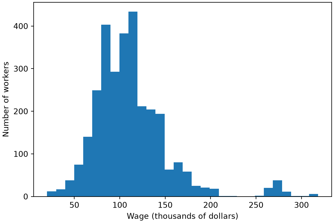
Figure 1: Bars counting the workers at each wage, in thousands of dollars.
import matplotlib.pyplot as plt

fig, ax = plt.subplots(figsize=(6, 4), layout="constrained")
ax.hist(wage_eda_py["wage"], bins=30);
ax.set_xlabel("Wage (thousands of dollars)");
ax.set_ylabel("Number of workers");
plt.show()

Histogram of wages in thousands of dollars of 3000 workers, with a peak near 100, a long right tail and a small separate group of workers near 270.

library(ggplot2) # nolint: undesirable_function_linter

wage_histogram <- wage_eda_r |>
  ggplot() +
  aes(wage) +
  geom_histogram(bins = 30) +
  labs(x = "Wage (thousands of dollars)", y = "Number of workers")
wage_histogram

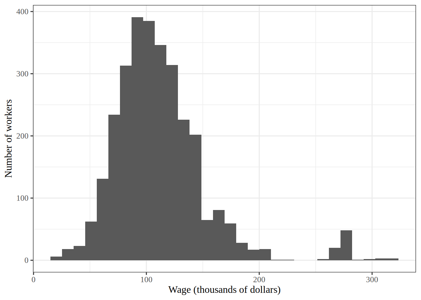
Histogram of wages in thousands of dollars of 3000 workers, with a peak near 100, a long right tail and a small separate group of workers near 270.

Show code
wage_eda_r_per_bin <- nrow(wage_eda_r) / 30

Figure 1 shows a peak near 100 thousand dollars and a long right tail.

I chose 30 bins, which is 100 workers per bar on average. Far fewer bins would hide the long right tail inside a few wide bars, and far more would leave most bars in the tail with one or two workers, so the outline would look ragged. That is why 30 is a compromise between the two.

ExrExercise 5 (Lab: wage against age)

Exercise 5 (Lab: wage against age) Use the Wage data. Draw a scatterplot of wage against age.

TipHint

Draw a scatterplot of one column against another, as in the plot of acceleration against horsepower in the primer.

Solution 5. This solution continues Solution 4.

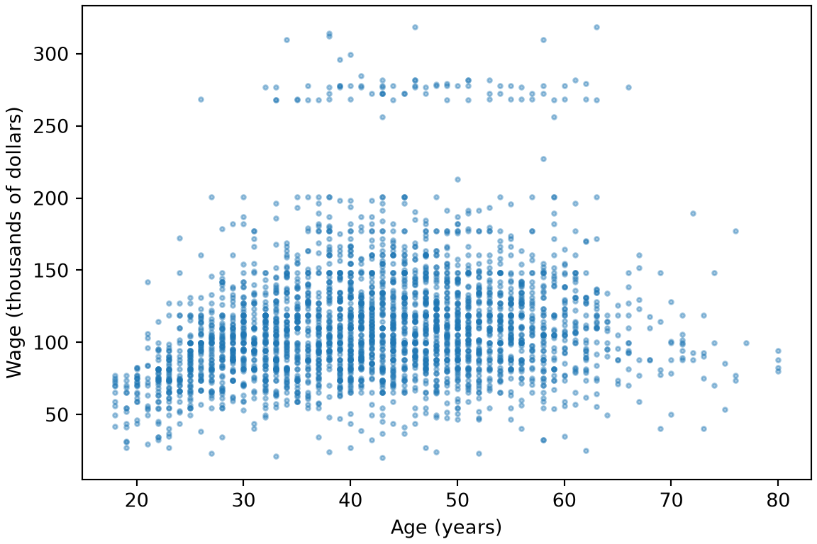
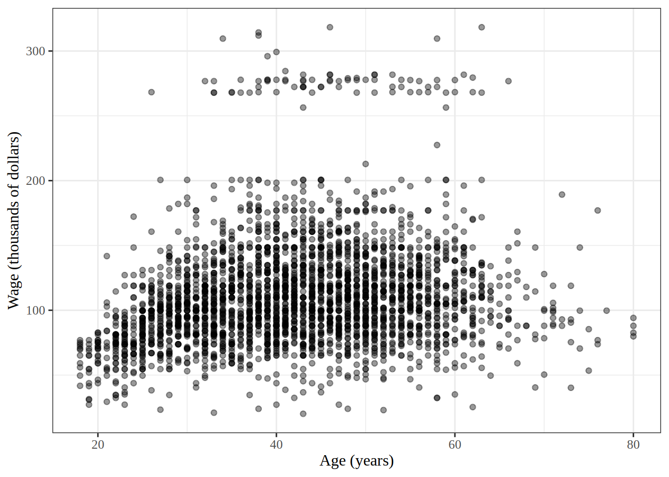
Figure 2: Wage, in thousands of dollars, against age in years, with one dot per worker.
fig, ax = plt.subplots(figsize=(6, 4), layout="constrained")
ax.scatter(wage_eda_py["age"], wage_eda_py["wage"], s=5, alpha=0.4);
ax.set_xlabel("Age (years)");
ax.set_ylabel("Wage (thousands of dollars)");
plt.show()

Scatterplot of wage in thousands of dollars against age in years for 3000 workers. Wages rise through the twenties and thirties, level off in middle age and then fall slightly, with a separate band of wages near 270 for ages 25 to 65.

wage_age_plot <- wage_eda_r |>
  ggplot() +
  aes(age, wage) +
  geom_point(alpha = 0.4) +
  labs(x = "Age (years)", y = "Wage (thousands of dollars)")
wage_age_plot

Scatterplot of wage in thousands of dollars against age in years for 3000 workers. Wages rise through the twenties and thirties, level off in middle age and then fall slightly, with a separate band of wages near 270 for ages 25 to 65.

In Figure 2, wage rises and then levels off or falls with age, so a straight line describes this relationship poorly, and that is why the next exercises use curves.

ExrExercise 6 (Lab: plots of every two columns)

Exercise 6 (Lab: plots of every two columns) Use the Wage data. Draw a plot of every two different columns among age, year, education and wage, in one grid.

TipHint

In R, the ggpairs() function of the GGally package draws all those plots in one grid, even with education as categories. In Python, the scatter_matrix() function of pandas.plotting draws them for numbers only, so turn education into its level number first.

Solution 6. This solution continues Solution 5.

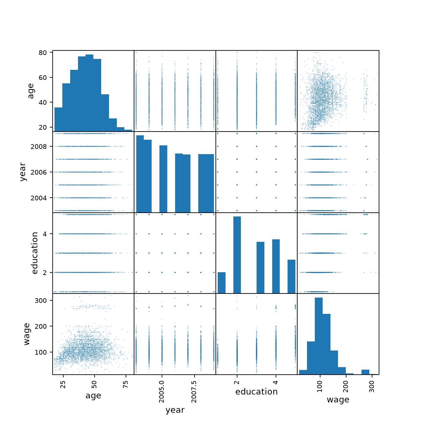
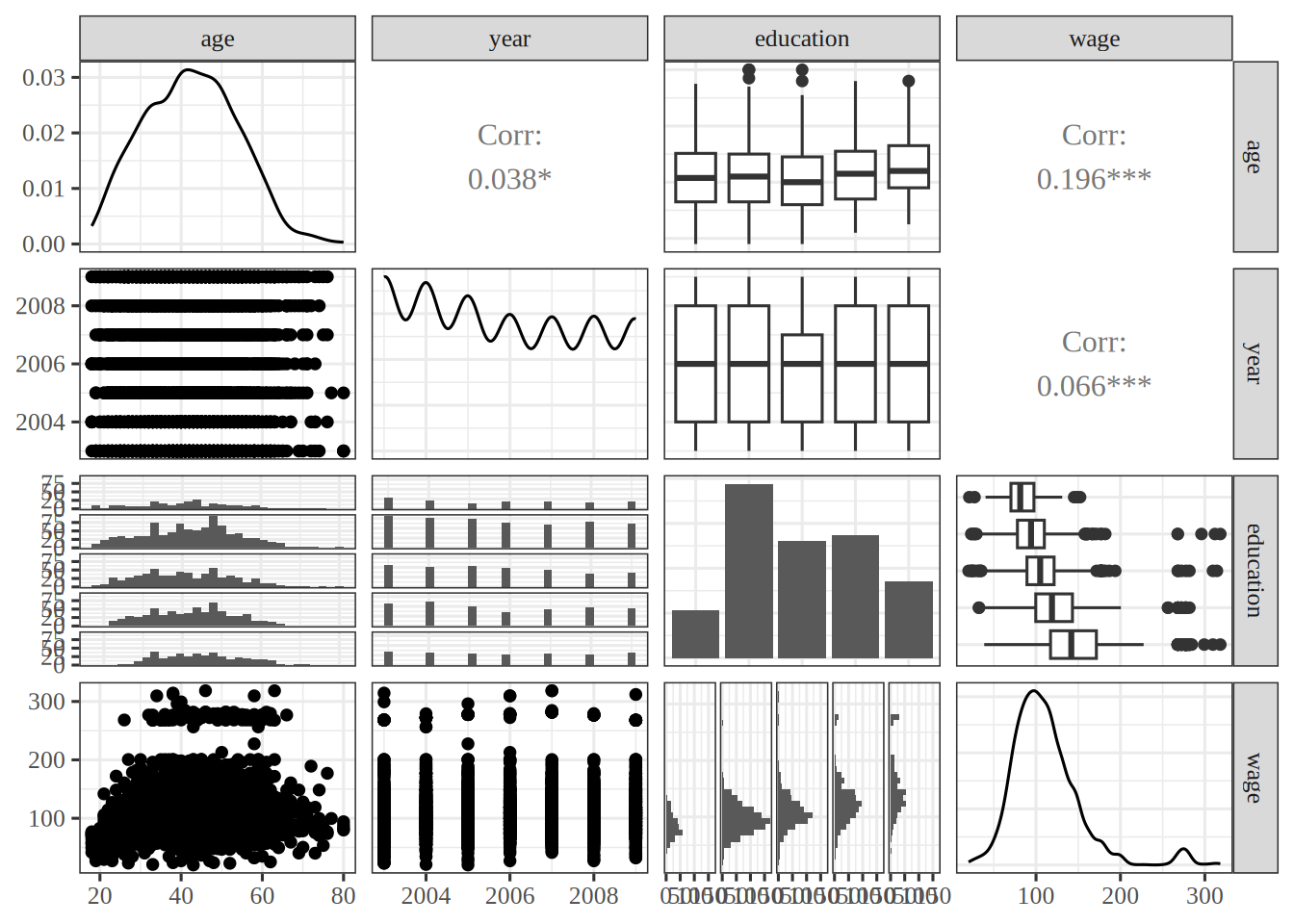
Figure 3: Plots of every two of age, year, education and wage.
from pandas.plotting import scatter_matrix

# the level number is the digit that starts each education category
education_level_py = wage_eda_py["education"].str[0].astype(int)
pairs_py = wage_eda_py[["age", "year", "wage"]].assign(
    education=education_level_py
)
scatter_matrix(
    pairs_py[["age", "year", "education", "wage"]], s=5, alpha=0.3, figsize=(7, 7)
);
plt.show()

Grid of scatterplots of every two of age, year, education level and wage, with a histogram of each column on the diagonal. Wage rises with education level and rises then levels off with age. Year takes only the seven values 2003 to 2009, and wage shifts only slightly from year to year.

library(GGally) # nolint: undesirable_function_linter

wage_pairs <- wage_eda_r |>
  select(age, year, education, wage) |>
  ggpairs()
wage_pairs

Grid of plots of every two of age, year, education and wage. The diagonal shows the distribution of each column. Off the diagonal, scatterplots and correlations pair the numeric columns, and boxplots and histograms split age, year and wage by education level. Wage rises with education and rises then levels off with age. Year takes only the seven values 2003 to 2009, and wage shifts only slightly from year to year.

In Figure 3, wage rises with each education level, and it bends with age as in Figure 2. Against year, wage shifts only a little. So wage is related to all three, most strongly to education and least to year.

ExrExercise 7 (Lab: wage against age and year together)

Exercise 7 (Lab: wage against age and year together) Use the Wage data. Draw a three-dimensional scatterplot of wage against age and year, with every year of the data.

TipHint

The plotly example in the programming primer draws a cloud of dots in 3D, with plot_ly() in R and go.Scatter3d() in Python. Turn the plot until you look along the year axis, and then along the age axis.

Solution 7. This solution continues Solution 6.

Figure 4: Wage, in thousands of dollars, against age in years and year, with one dot per worker.
import html
import plotly.graph_objects as go

wage_cloud_py = go.Figure(
    go.Scatter3d(
        x=wage_eda_py["age"],
        y=wage_eda_py["year"],
        z=wage_eda_py["wage"],
        mode="markers",
        marker=dict(size=2, opacity=0.5),
    )
)
# an orthographic view keeps the slices parallel when the plot is turned
wage_cloud_py.update_layout(
    scene=dict(
        xaxis_title="age (years)",
        yaxis_title="year",
        zaxis_title="wage (thousands of dollars)",
        camera=dict(projection=dict(type="orthographic")),
    ),
);
print(
    "```{=html}\n"
    + f'<div role="group" aria-label="{html.escape(r.wage_cloud_alt)}">\n'
    + wage_cloud_py.to_html(full_html=False, include_plotlyjs="cdn")
    + "\n</div>\n```"
)
# an orthographic view keeps the slices parallel when the plot is turned
wage_cloud_projection <- list(type = "orthographic")
wage_cloud_camera <- list(projection = wage_cloud_projection)
wage_cloud_xaxis <- list(title = "age (years)")
wage_cloud_yaxis <- list(title = "year")
wage_cloud_zaxis <- list(title = "wage (thousands of dollars)")
wage_cloud_scene <- list(
  xaxis = wage_cloud_xaxis,
  yaxis = wage_cloud_yaxis,
  zaxis = wage_cloud_zaxis,
  camera = wage_cloud_camera
)
wage_cloud_marker <- list(size = 2, opacity = 0.5)
wage_eda_r |>
  plotly::plot_ly(x = ~age, y = ~year, z = ~wage) |>
  plotly::add_markers(marker = wage_cloud_marker) |>
  plotly::layout(scene = wage_cloud_scene)

Turning Figure 4 to look along each axis shows:

  • Along the year axis: the seven slices from 2003 to 2009 lie on top of one another, and each has the same rise and leveling off with age.
  • Along the age axis: the later slices sit slightly higher. The mean wage is 106.2 thousand dollars in 2003 and 116.0 thousand in 2009.

So the curve in age keeps its shape from year to year, and year shifts it up by about 10 thousand dollars over the seven years. A model that adds a curve in age to a term in year matches that picture.

3 Polynomials and step functions

ExrExercise 8 (Lab: predict a wage with a polynomial)

Exercise 8 (Lab: predict a wage with a polynomial) Download the Wage data from data/wage.csv, which has the wage (in thousands of dollars) and age of \(3000\) male workers in the Mid-Atlantic United States [1]. Fit a polynomial regression of wage on age of degree \(4\), and use it to predict the wage of a \(50\)-year-old.

TipHint

The np.polyfit and np.polyval functions fit and evaluate a polynomial of a chosen degree. In R, poly() supplies the polynomial columns that lm() uses.

Solution 8.

import pandas as pd
from sklearn.linear_model import LinearRegression
from sklearn.pipeline import make_pipeline
from sklearn.preprocessing import PolynomialFeatures, StandardScaler

wage_py = pd.read_csv("data/wage.csv")
age_py = wage_py[["age"]]
age_50_py = pd.DataFrame({"age": [50]})
poly_basis_py = PolynomialFeatures(degree=4)
poly_py = make_pipeline(StandardScaler(), poly_basis_py, LinearRegression())
poly_py.fit(age_py, wage_py["wage"])
Pipeline(steps=[('standardscaler', StandardScaler()),
                ('polynomialfeatures', PolynomialFeatures(degree=4)),
                ('linearregression', LinearRegression())])
In a Jupyter environment, please rerun this cell to show the HTML representation or trust the notebook.
On GitHub, the HTML representation is unable to render, please try loading this page with nbviewer.org.
pred_poly_py = poly_py.predict(age_50_py)[0]
pred_poly_py
np.float64(119.57013127056274)
wage <- readr::read_csv("data/wage.csv", show_col_types = FALSE)
new_age <- tibble(age = 50)
poly_fit <- linear_reg() |>
  fit(wage ~ poly(age, 4), data = wage)
poly_pred <- predict(poly_fit, new_data = new_age)
pred_poly_r <- poly_pred$.pred
pred_poly_r
[1] 119.5701

The predicted wage of a \(50\)-year-old is 119.6 thousand dollars in the R run and 119.6 in the Python run.

ExrExercise 9 (Lab: print the coefficients of a degree-4 polynomial)

Exercise 9 (Lab: print the coefficients of a degree-4 polynomial) Fit a polynomial regression of wage on age of degree \(4\) in the Wage data, and print a table of its coefficients, with their standard errors and \(p\)-values.

TipHint

In Python, pass the formula wage ~ age + I(age**2) + I(age**3) + I(age**4) to smf.ols(), and the fit’s summary2() holds the table. In R, the formula wage ~ poly(age, 4, raw = TRUE) gives the same fit, and summary() or tidy() gives the table. In a tidymodels recipe, step_poly() builds the same terms when its options list holds raw = TRUE.

Solution 9.

Show code
import numpy as np
import pandas as pd
import statsmodels.formula.api as smf

Wage = pd.read_csv("data/wage.csv")
y = Wage["wage"]
age = Wage["age"]
# the powers 1 to 4 of age span the same space as ISLP's poly() basis
poly_formula = "wage ~ age + I(age**2) + I(age**3) + I(age**4)"
M = smf.ols(poly_formula, Wage).fit()
age_coef_py = M.params["age"]
M.summary2().tables[1].iloc[:, :4]
                  Coef.   Std.Err.         t     P>|t|
Intercept   -184.154180  60.040377 -3.067172  0.002180
age           21.245521   5.886748  3.609042  0.000312
I(age ** 2)   -0.563859   0.206108 -2.735743  0.006261
I(age ** 3)    0.006811   0.003066  2.221409  0.026398
I(age ** 4)   -0.000032   0.000016 -1.951938  0.051039
Show code
rec_poly <- recipe(wage ~ age, data = wage) |>
  step_poly(age, degree = 4)

lm_spec <- linear_reg() |>
  set_mode("regression") |>
  set_engine("lm")

poly_wf <- workflow() |>
  add_model(lm_spec) |>
  add_recipe(rec_poly)

poly_fit <- fit(poly_wf, data = wage)
tidy(poly_fit)
Show code
# poly() builds an orthogonal basis unless raw = TRUE
poly(1:6, degree = 4, raw = FALSE)
              1          2          3          4
[1,] -0.5976143  0.5455447 -0.3726780  0.1889822
[2,] -0.3585686 -0.1091089  0.5217492 -0.5669467
[3,] -0.1195229 -0.4364358  0.2981424  0.3779645
[4,]  0.1195229 -0.4364358 -0.2981424  0.3779645
[5,]  0.3585686 -0.1091089 -0.5217492 -0.5669467
[6,]  0.5976143  0.5455447  0.3726780  0.1889822
attr(,"coefs")
attr(,"coefs")$alpha
[1] 3.5 3.5 3.5 3.5

attr(,"coefs")$norm2
[1]  1.00000  6.00000 17.50000 37.33333 64.80000 82.28571

attr(,"degree")
[1] 1 2 3 4
attr(,"class")
[1] "poly"   "matrix"
Show code
poly(1:6, degree = 4, raw = TRUE)
     1  2   3    4
[1,] 1  1   1    1
[2,] 2  4   8   16
[3,] 3  9  27   81
[4,] 4 16  64  256
[5,] 5 25 125  625
[6,] 6 36 216 1296
attr(,"degree")
[1] 1 2 3 4
attr(,"class")
[1] "poly"   "matrix"
Show code
raw_options <- list(raw = TRUE)
rec_raw_poly <- recipe(wage ~ age, data = wage) |>
  step_poly(age, degree = 4, options = raw_options)

raw_poly_wf <- workflow() |>
  add_model(lm_spec) |>
  add_recipe(rec_raw_poly)

raw_poly_fit <- fit(raw_poly_wf, data = wage)

poly_coefs <- tidy(raw_poly_fit)
poly_coefs
Show code
poly_lm <- lm(wage ~ poly(age, 4, raw = TRUE), data = wage)
poly_lm_summary <- summary(poly_lm)
poly_lm_summary$coefficients
                               Estimate   Std. Error   t value     Pr(>|t|)
(Intercept)               -1.841542e+02 6.004038e+01 -3.067172 0.0021802539
poly(age, 4, raw = TRUE)1  2.124552e+01 5.886748e+00  3.609042 0.0003123618
poly(age, 4, raw = TRUE)2 -5.638593e-01 2.061083e-01 -2.735743 0.0062606446
poly(age, 4, raw = TRUE)3  6.810688e-03 3.065931e-03  2.221409 0.0263977518
poly(age, 4, raw = TRUE)4 -3.203830e-05 1.641359e-05 -1.951938 0.0510386498

All three tabs fit the same polynomial in age, and they give the same coefficients: the coefficient of age is 21.25 in the tidymodels run, 21.25 in the base R run and 21.25 in the Python run. The book’s lab uses ISLP’s poly() instead, which, like R’s poly() without raw = TRUE, builds an orthogonal basis for it. That basis gives the same fitted values, but different coefficients and \(p\)-values. The tidymodels tab fits it both ways: step_poly() uses the orthogonal basis unless its options list holds raw = TRUE.

ExrExercise 10 (Lab: build a grid of ages)

Exercise 10 (Lab: build a grid of ages) Build a grid of \(100\) evenly spaced ages, from the youngest worker’s age in the Wage data to the oldest’s, and store it in a data frame under the name age.

Solution 10.

Show code
age_grid = np.linspace(age.min(),
                       age.max(),
                       100)
age_df = pd.DataFrame({'age': age_grid})
age_df
          age
0   18.000000
1   18.626263
2   19.252525
3   19.878788
4   20.505051
..        ...
95  77.494949
96  78.121212
97  78.747475
98  79.373737
99  80.000000

[100 rows x 1 columns]
Show code
age_min <- min(wage$age)
age_max <- max(wage$age)
age_seq <- seq(age_min, age_max, length.out = 100)
age_range <- tibble(age = age_seq)
age_range
Show code
age_limits <- range(wage$age)
grid_ages <- seq(age_limits[1], age_limits[2], length.out = 100)
# This tab uses base R's data frame
age_grid <- data.frame(age = grid_ages) # nolint: undesirable_function_linter.
head(age_grid)

The grid runs from age 18 to age 80.

ExrExercise 11 (Lab: write a helper that plots a fit with confidence bands)

Exercise 11 (Lab: write a helper that plots a fit with confidence bands) Write a helper that fits a regression of wage in the Wage data, predicts on the grid of Exercise 10, and plots the data with the fitted curve with \(95\%\) confidence bands.

TipHint

In Python, a function that takes a formula can fit it with smf.ols(), and the fit’s get_prediction() gives the bands. In R, predict() gives the bands: with interval = "confidence" for an lm() fit, and with type = "conf_int" for a tidymodels workflow after fit().

Solution 11.

Show code
import matplotlib.pyplot as plt


def plot_wage_fit(age_df,
                  formula,
                  title):

    M = smf.ols(formula, Wage).fit()
    preds = M.get_prediction(age_df)
    bands = preds.conf_int(alpha=0.05)
    fig, ax = plt.subplots(figsize=(6, 4), layout="constrained")
    ax.scatter(age,
               y,
               facecolor='gray',
               alpha=0.5)
    for val, ls in zip([preds.predicted_mean,
                        bands[:, 0],
                        bands[:, 1]],
                       ['b', 'r--', 'r--']):
        ax.plot(age_df.values, val, ls, linewidth=3)
    ax.set_title(title)
    ax.set_xlabel('Age')
    ax.set_ylabel('Wage')
    return ax
Show code
# lds has no R/ directory, and wage is the page's data:
# nolint start: function_location_linter, object_usage_linter.
plot_wage_wf <- function(rec, new_data, title) {
  wf_fit <- workflow() |>
    add_model(lm_spec) |>
    add_recipe(rec) |>
    fit(data = wage)
  fitted_curve <- augment(wf_fit, new_data = new_data)
  bands <- predict(wf_fit, new_data = new_data, type = "conf_int")
  regression_lines <- bind_cols(fitted_curve, bands)

  wage |>
    ggplot() +
    aes(x = age, y = wage) +
    geom_point(alpha = 0.2) +
    geom_line(aes(y = .pred), color = "darkgreen",
              data = regression_lines) +
    geom_line(aes(y = .pred_lower), data = regression_lines,
              linetype = "dashed", color = "blue") +
    geom_line(aes(y = .pred_upper), data = regression_lines,
              linetype = "dashed", color = "blue") +
    labs(title = title, x = "Age", y = "Wage")
}
# nolint end
Show code
# lds has no R/ directory, and wage is the page's data:
# nolint start: function_location_linter, object_usage_linter.
line_types <- c(1, 2, 2)
line_colors <- c("blue", "red", "red")
plot_wage_fit <- function(formula, new_data, title) {
  fit <- lm(formula, data = wage)
  bands <- predict(fit, newdata = new_data, interval = "confidence")
  # "#BEBEBE80" is gray at half opacity
  plot(wage$age, wage$wage, col = "#BEBEBE80", pch = 20,
       xlab = "Age", ylab = "Wage", main = title)
  matlines(new_data$age, bands, lty = line_types,
           col = line_colors, lwd = 3)
  invisible(bands)
}
# nolint end

The alpha setting of ax.scatter() and of geom_point() makes each marker partly transparent, so a dark area shows where many workers are; in base R, the last two digits of the color "#BEBEBE80" do the same. In Python, zip() matches the fitted curve and the two bands with their colors and line types for the for loop. In base R, predict() with interval = "confidence" returns the curve and the two bands side by side in one matrix, and matlines() draws a line for each of the three. The tidymodels helper takes a recipe rather than a formula, and gets the bands from predict() with type = "conf_int".

ExrExercise 12 (Lab: plot the degree-4 polynomial fit)

Exercise 12 (Lab: plot the degree-4 polynomial fit) Use the helper of Exercise 11 to plot the polynomial fit of Exercise 9, with its \(95\%\) confidence bands.

Solution 12.

Show code
plot_wage_fit(age_df,
              poly_formula,
              'Degree-4 Polynomial');
plt.show()
Show code
plot_wage_wf(rec_poly, age_range, "Degree-4 Polynomial")
Show code
poly4_bands <- plot_wage_fit(wage ~ poly(age, 4), age_grid,
                             "Degree-4 Polynomial")
Show code
poly4_peak <- age_grid$age[which.max(poly4_bands[, "fit"])]
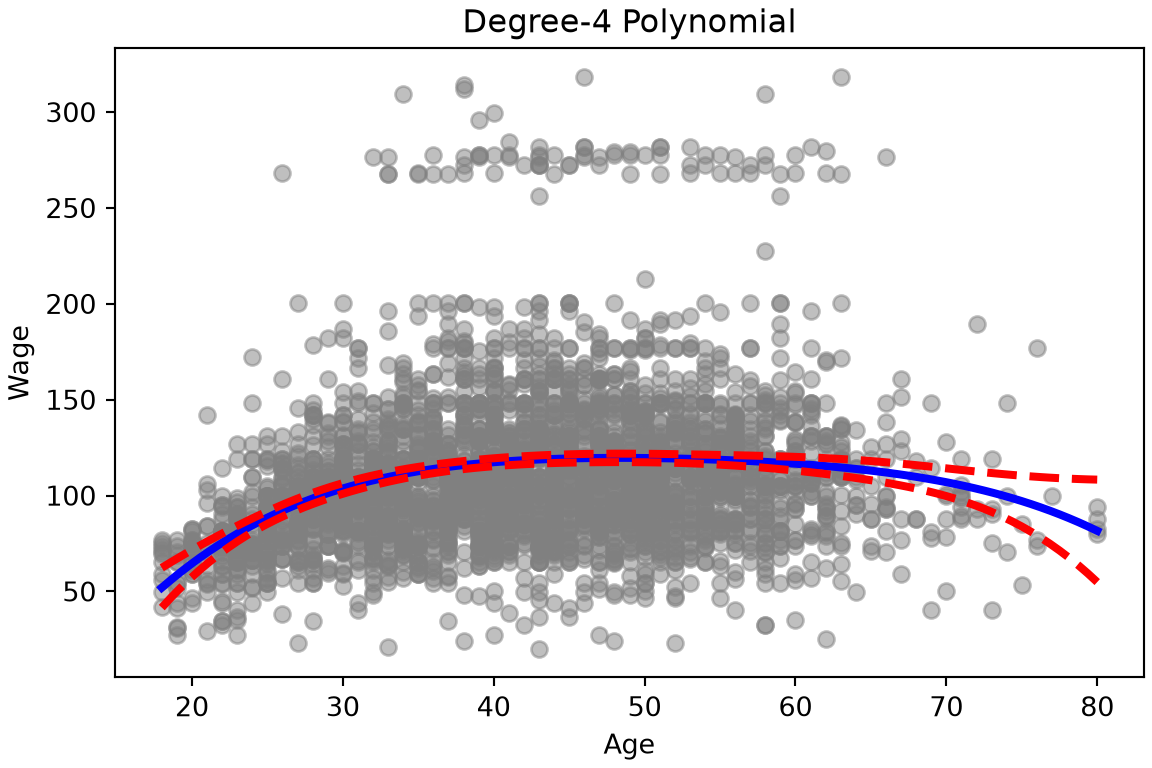
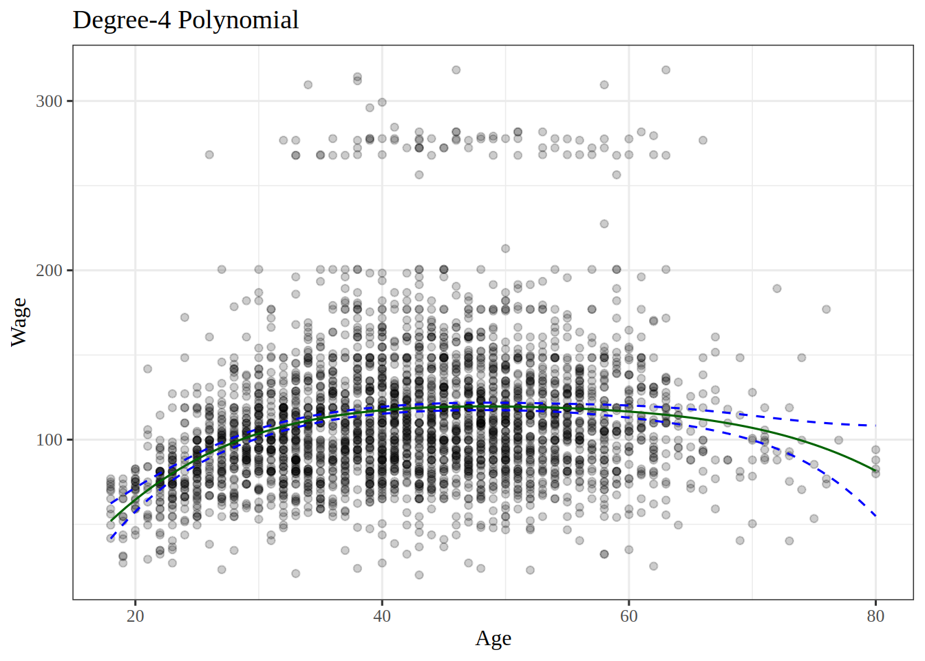
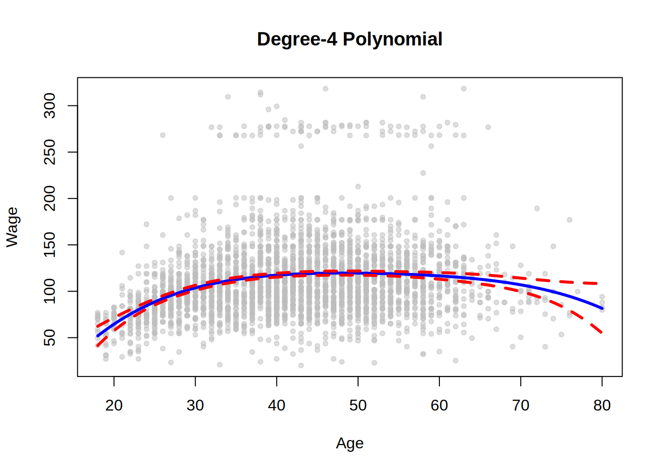
Figure 5: Wage against age, with the degree-4 polynomial fit and its \(95\%\) confidence bands.

In Figure 5, the fitted wage rises until about age 48, and then falls. The bands are narrow through middle age and widen past age \(70\), where there are few workers.

ExrExercise 13 (Lab: choose a polynomial degree by ANOVA)

Exercise 13 (Lab: choose a polynomial degree by ANOVA) With polynomial regression we must decide on the degree of the polynomial to use. The Wage data in data/wage.csv record the wage (in thousands of dollars) and age of \(3000\) male workers in the Mid-Atlantic United States [1].

Fit polynomial models of wage in age of degrees 1 through 5, and use partial \(F\)-tests of each model against the one before it to decide which degree is enough.

TipHint

The five models are nested. The tidymodels example in the programming primer compares such models: anova_lm() from statsmodels.stats.anova takes the smf.ols() fits in order in Python, and anova() takes the lm() fits in order in R.

Solution 13.

Show code
import pandas as pd
import statsmodels.formula.api as smf
from statsmodels.stats.anova import anova_lm

Wage = pd.read_csv("data/wage.csv")
# the degree-d model has the powers 1 through d of age,
# so each model contains the one before it
powers = [f"I(age**{k})" for k in range(1, 6)]
formulas = ["wage ~ " + " + ".join(powers[:d]) for d in range(1, 6)]
models = [smf.ols(formula, Wage).fit() for formula in formulas]
# each row tests a model against the row above it
degree_anova_py = anova_lm(*models)
degree_anova_py
   df_resid           ssr  df_diff        ss_diff           F        Pr(>F)
0    2998.0  5.022216e+06      0.0            NaN         NaN           NaN
1    2997.0  4.793430e+06      1.0  228786.010128  143.593107  2.363850e-32
2    2996.0  4.777674e+06      1.0   15755.693664    9.888756  1.679202e-03
3    2995.0  4.771604e+06      1.0    6070.152124    3.809813  5.104620e-02
4    2994.0  4.770322e+06      1.0    1282.563017    0.804976  3.696820e-01
Show code
wage_deg <- readr::read_csv("data/wage.csv", show_col_types = FALSE)
# the degree-d model is a polynomial of degree d in age,
# so each model contains the one before it
degree_fits <- purrr::map(1:5, \(d) lm(wage ~ poly(age, d), data = wage_deg))
# each row tests a model against the row above it
degree_anova <- rlang::exec(anova, !!!degree_fits) |> tidy()
degree_anova

The * in Python and the !!! in R hand each model in the list to the test one by one.

The \(p\)-value comparing degree 1 with degree 2 is essentially zero (2.4e-32 in R). Degree 2 against degree 3 gives 0.0017, and degree 3 against degree 4 gives 0.051, roughly 5%. Degree 5 is unnecessary (\(p\) = 0.37). The Python run gives the same \(p\)-values, 2.4e-32, 0.0017, 0.051 and 0.37.

Either a polynomial of degree 3 or one of degree 4 gives a reasonable fit.

ExrExercise 14 (Lab: choose the degree with education in the models)

Exercise 14 (Lab: choose the degree with education in the models) In Exercise 13, each model of wage in the Wage data held a polynomial in age alone. Workers’ education also varies, as a categorical variable with five levels.

Repeat the partial \(F\)-tests of Exercise 13, but with education included in each model alongside a polynomial in age of degrees 1, 2 and 3.

TipHint

In a formula, education becomes one indicator per category after the first, in smf.ols() in Python and in lm() in R. Compare the fits with anova_lm() in Python and anova() in R, as in the tidymodels example in the programming primer.

Solution 14.

Show code
# education is text, so the formula gives it one column per category;
# every model has those columns, and the degree in age grows from 1 to 3
powers = [f"I(age**{k})" for k in range(1, 4)]
formulas = ["wage ~ education + " + " + ".join(powers[:d]) for d in range(1, 4)]
models = [smf.ols(formula, Wage).fit() for formula in formulas]
education_anova_py = anova_lm(*models)
education_anova_py
   df_resid           ssr  df_diff        ss_diff           F        Pr(>F)
0    2994.0  3.867992e+06      0.0            NaN         NaN           NaN
1    2993.0  3.725395e+06      1.0  142597.097010  114.696898  2.728001e-26
2    2992.0  3.719809e+06      1.0    5586.660322    4.493588  3.410431e-02
Show code
wage_edu <- readr::read_csv("data/wage.csv", show_col_types = FALSE)
# education is text, so lm() gives it one column per category;
# every model has those columns, and the degree in age grows from 1 to 3
education_formulas <- purrr::map(1:3, \(d) wage ~ education + poly(age, d))
education_fits <- purrr::map(education_formulas, lm, data = wage_edu)
education_anova <- rlang::exec(anova, !!!education_fits) |> tidy()
education_anova

With education in the models, the \(p\)-value of degree 2 against degree 1 is 2.7e-26, and the \(p\)-value of degree 3 against degree 2 is 0.03 (2.7e-26 and 0.03 in Python). So degree 2 clearly improves on degree 1, and degree 3 improves on degree 2 only at the 5% level.

The tests work whether or not the polynomials are orthogonal, provided the models are nested: R’s poly() builds orthogonal polynomials, while the Python code uses age, age**2 and age**3 as they are, and the two runs give the same \(p\)-values. As an alternative, we could choose the polynomial degree by cross-validation.

ExrExercise 15 (Lab: predict a high wage with a logistic polynomial)

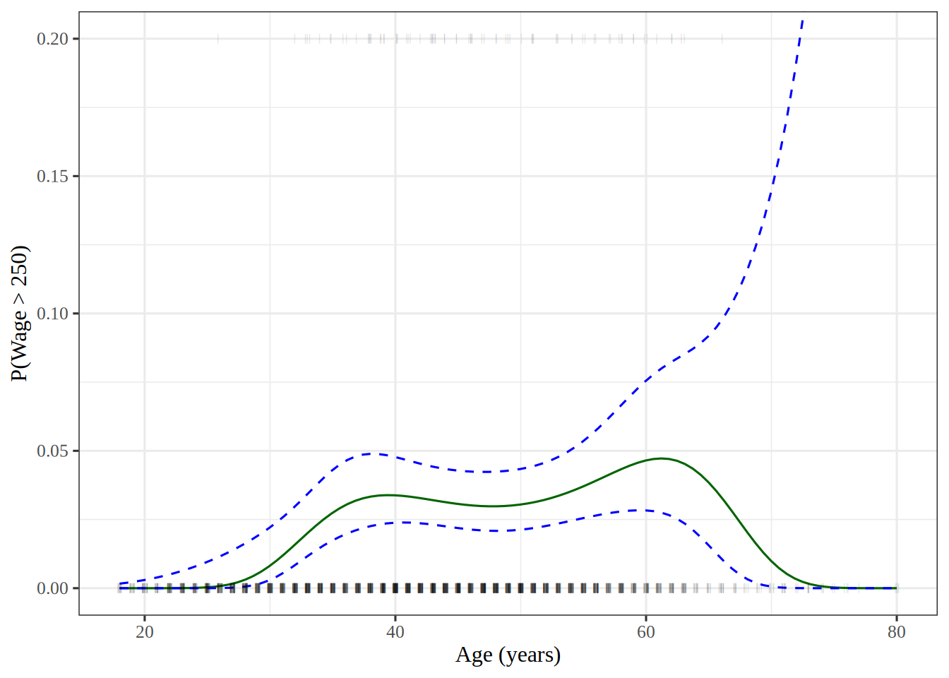
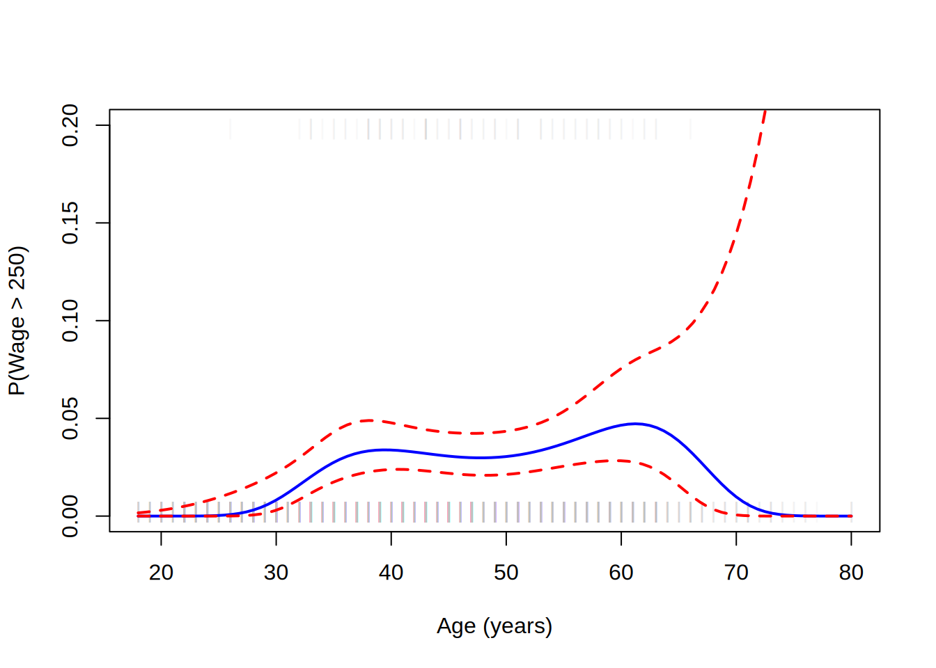
Exercise 15 (Lab: predict a high wage with a logistic polynomial) Now model whether a worker in the Wage data earns more than $250,000 per year, that is, whether wage > 250, since wage is in thousands of dollars.

Fit a logistic regression of wage > 250 on a polynomial of degree \(4\) in age, and plot the predicted probability against age, with \(95\%\) confidence bands and a rug plot of the workers.

TipHint

The GLM example in the programming primer fits a logistic regression: smf.glm() with a Binomial family in Python, and logistic_reg() or glm() in R. get_prediction() in Python and predict() with se.fit = TRUE in R give the standard errors that the bands need, and in a tidymodels workflow, predict() with type = "conf_int" gives the bands themselves. A rug plot marks each worker’s age with a short tick, at the top of the plot for the workers above $250,000 and at the bottom for the rest.

Solution 15.

Show code
import matplotlib.pyplot as plt
import numpy as np
import pandas as pd
import statsmodels.api as sm
import statsmodels.formula.api as smf

Wage = pd.read_csv("data/wage.csv")
y = Wage["wage"]
age = Wage["age"]
# 1 or 0, since a True/False column would make the formula model P(False)
high_earn = Wage["high_earn"] = (y > 250).astype(int)
# a degree-4 polynomial in age on the log-odds scale
powers = " + ".join(f"I(age**{k})" for k in range(1, 5))
glm = smf.glm("high_earn ~ " + powers, Wage, family=sm.families.Binomial())
B = glm.fit()
# predict on a grid of 100 ages that spans the observed range
age_df = pd.DataFrame({"age": np.linspace(age.min(), age.max(), 100)})
preds = B.get_prediction(age_df)
bands = preds.conf_int(alpha=0.05)

fig, ax = plt.subplots(figsize=(6, 4), layout="constrained")
# faint marks, so that darker marks show ages that many workers share
rug_y = np.where(high_earn, 0.198, 0.002)
ax.scatter(age, rug_y, c="gray", marker="|", alpha=0.1);
ax.plot(age_df["age"], preds.predicted_mean, "b", linewidth=2);
ax.plot(age_df["age"], bands, "r--", linewidth=2);
ax.set_xlabel("Age (years)");
ax.set_ylim([0, 0.2]);
ax.set_ylabel("P(Wage > 250)");
plt.show()
Show code
high_levels <- c(TRUE, FALSE)
high_labels <- c("High", "Low")
wage_hl <- wage |>
  mutate(high = factor(wage > 250, levels = high_levels, labels = high_labels))

rec_poly_high <- recipe(high ~ age, data = wage_hl) |>
  step_poly(age, degree = 4)

lr_spec <- logistic_reg() |>
  set_engine("glm") |>
  set_mode("classification")

lr_poly_wf <- workflow() |>
  add_model(lr_spec) |>
  add_recipe(rec_poly_high)

lr_poly_fit <- fit(lr_poly_wf, data = wage_hl)

# predict on a grid of 100 ages that spans the observed range
age_lo <- min(wage_hl$age)
age_hi <- max(wage_hl$age)
age_seq_hl <- seq(age_lo, age_hi, length.out = 100)
high_grid <- tibble(age = age_seq_hl)
high_probs <- augment(lr_poly_fit, new_data = high_grid)
high_bands <- predict(lr_poly_fit, new_data = high_grid, type = "conf_int")
regression_lines <- bind_cols(high_probs, high_bands)

y_window <- c(0, 0.2)
regression_lines |>
  ggplot() +
  aes(x = age) +
  geom_line(aes(y = .pred_High), color = "darkgreen") +
  geom_line(aes(y = .pred_lower_High), color = "blue", linetype = "dashed") +
  geom_line(aes(y = .pred_upper_High), color = "blue", linetype = "dashed") +
  geom_jitter(aes(y = (high == "High") / 5), data = wage_hl,
              shape = "|", height = 0, width = 0.2, alpha = 0.1) +
  coord_cartesian(ylim = y_window) +
  labs(x = "Age (years)", y = "P(Wage > 250)")
Show code
wage_hi <- wage
wage_hi$high_earn <- wage_hi$wage > 250
# a degree-4 polynomial in age on the log-odds scale
high_fit <- glm(high_earn ~ poly(age, 4), family = binomial, data = wage_hi)
# predict on a grid of 100 ages that spans the observed range
age_range <- range(wage_hi$age)
grid_ages <- seq(age_range[1], age_range[2], length.out = 100)
# This tab uses base R's data frame
logit_grid <- data.frame(age = grid_ages) # nolint: undesirable_function_linter.
# compute the band on the log-odds scale, then map it to probabilities
link_pred <- predict(high_fit, logit_grid, type = "link", se.fit = TRUE)
z_crit <- qnorm(0.975)
lower_link <- link_pred$fit - z_crit * link_pred$se.fit
upper_link <- link_pred$fit + z_crit * link_pred$se.fit
fit_prob <- plogis(link_pred$fit)
lower_prob <- plogis(lower_link)
upper_prob <- plogis(upper_link)
# cbind() makes the matrix whose columns matlines() draws
# nolint start: undesirable_function_linter.
high_curve <- cbind(fit_prob, lower_prob, upper_prob)
# nolint end
peak_age <- grid_ages[which.max(fit_prob)]

# faint marks, so that darker marks show ages that many workers share
rug_y <- 0.002 + 0.196 * wage_hi$high_earn
y_window <- c(0, 0.2)
band_types <- c(1, 2, 2)
band_colors <- c("blue", "red", "red")
plot(wage_hi$age, rug_y, pch = "|", col = "#BEBEBE1A", ylim = y_window,
     xlab = "Age (years)", ylab = "P(Wage > 250)")
matlines(grid_ages, high_curve, lty = band_types, col = band_colors, lwd = 2)
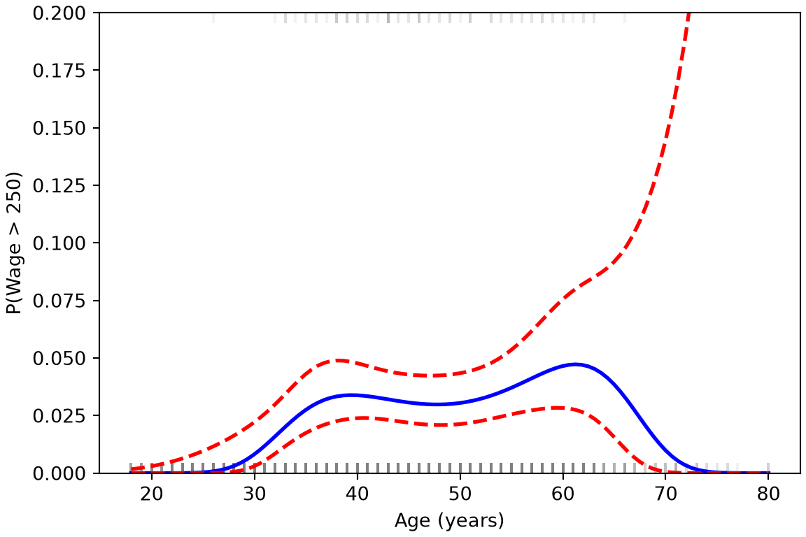
Figure 6: Predicted probability that a worker’s wage exceeds \(250\) thousand dollars, against age, with \(95\%\) confidence bands.

The double assignment high_earn = Wage["high_earn"] = ... in Python both binds the variable high_earn and stores the indicator in the Wage data frame under that name, as mutate() does in the tidymodels tab. A tidymodels classifier needs a factor outcome, so that tab codes each wage as High or Low, with High as the first level so that .pred_High is the probability of a high wage. Only 79 of the 3000 workers earn more than $250,000.

In Figure 6, the workers who earn more than $250,000 are the gray marks at the top of the plot, and the other workers are the gray marks at the bottom. Each mark of this rug plot is faint, so a dark mark shows an age that many workers share. The predicted probability stays near zero through the twenties, stays low through middle age, and is highest at age 61 in the base R run. The upper confidence band rises steeply at the oldest ages, where there are few workers.

ExrExercise 16 (Lab: predict a wage with a step function)

Exercise 16 (Lab: predict a wage with a step function) Split the observed ages into \(4\) age ranges that each contain the same number of years. Fit a regression of wage on age that gives every worker in an age range the same fitted value, and use it to predict the wage of a \(50\)-year-old.

TipHint

The pd.cut function assigns each value to an interval, with edges from np.quantile, and a group mean gives the value of each range. In R, cut() assigns each value to an interval, with edges from quantile(); in a tidymodels recipe, step_cut() does the same.

Solution 16.

from sklearn.linear_model import LinearRegression
from sklearn.pipeline import make_pipeline
from sklearn.preprocessing import KBinsDiscretizer

bins_py = KBinsDiscretizer(n_bins=4, encode="onehot-dense", strategy="uniform")
step_py = make_pipeline(bins_py, LinearRegression())
step_py.fit(age_py, wage_py["wage"])
Pipeline(steps=[('kbinsdiscretizer',
                 KBinsDiscretizer(encode='onehot-dense', n_bins=4,
                                  strategy='uniform')),
                ('linearregression', LinearRegression())])
In a Jupyter environment, please rerun this cell to show the HTML representation or trust the notebook.
On GitHub, the HTML representation is unable to render, please try loading this page with nbviewer.org.
pred_step_py = step_py.predict(age_50_py)[0]
pred_step_py
np.float64(118.04412419616096)
age_lo <- min(wage$age)
age_hi <- max(wage$age)
cut_edges <- seq(age_lo, age_hi, length.out = 5)
# step_cut() adds the outer edges itself
inner_edges <- cut_edges[2:4]
rec_cut <- recipe(wage ~ age, data = wage) |>
  step_cut(age, breaks = inner_edges)

lm_spec <- linear_reg() |>
  set_mode("regression") |>
  set_engine("lm")

cut_wf <- workflow() |>
  add_model(lm_spec) |>
  add_recipe(rec_cut)

cut_fit <- fit(cut_wf, data = wage)
cut_pred <- predict(cut_fit, new_data = new_age)
cut_pred
age_range <- range(wage$age)
age_breaks <- seq(age_range[1], age_range[2], length.out = 5)
step_formula <- wage ~ cut(
  age,
  breaks = age_breaks,
  right = FALSE,
  include.lowest = TRUE
)
step_fit <- lm(step_formula, data = wage)
pred_step_r <- predict(step_fit, newdata = new_age)
pred_step_r
       1 
118.0441 

The bins have edges 18, 33.5, 49, 64.5, 80, so a \(50\)-year-old falls in the third bin. The predicted wage is 117.8 thousand dollars in the tidymodels run, 118 in the base R run and 118 in the Python run. The tidymodels tab passes step_cut() only the three inner edges as its breaks, because step_cut() adds the youngest and oldest ages as the outer edges itself. step_cut() closes each bin on the right, so it puts the workers aged exactly \(49\) in the second bin, where cut() with right = FALSE and scikit-learn put them in the third; that moves the third bin’s sample mean wage a little.

ExrExercise 17 (Lab: fit a step function with quantile bins)

Exercise 17 (Lab: fit a step function with quantile bins) Split age into \(4\) bins at its sample quantiles \(0.25\), \(0.5\) and \(0.75\). Each bin then holds about the same number of workers. Fit a step function regression of wage on these bins, with one indicator for each bin and no intercept. What does each coefficient estimate?

TipHint

In Python, pd.qcut() cuts a variable at its quantiles, and pd.get_dummies() makes one 0-1 variable for each bin. In R, quantile() gives the cutpoints. cut() assigns each age to its bin, or step_discretize() does so in a tidymodels recipe, and a - 1 or 0 + after the ~ drops the intercept.

Solution 17.

Show code
import pandas as pd
import statsmodels.api as sm

cut_age = pd.qcut(wage_py["age"], 4)
# float indicators, one per bin, and no intercept
dummies_py = pd.get_dummies(cut_age, dtype=float)
step_q_py = sm.OLS(wage_py["wage"], dummies_py).fit()
step_q_py.params
(17.999, 33.75]     94.158392
(33.75, 42.0]      116.660810
(42.0, 51.0]       119.188665
(51.0, 80.0]       116.571716
dtype: float64
Show code
lm_spec <- linear_reg() |>
  set_mode("regression") |>
  set_engine("lm")

rec_discretize <- recipe(wage ~ age, data = wage) |>
  step_discretize(age, num_breaks = 4)

# 0 + drops the intercept, so there is one coefficient per bin
discretize_wf <- workflow() |>
  add_model(lm_spec, formula = wage ~ 0 + age) |>
  add_recipe(rec_discretize)

discretize_fit <- fit(discretize_wf, data = wage)
discretize_coefs <- tidy(discretize_fit)
discretize_coefs
Show code
# the trained step keeps the breaks it estimated
discretize_prepped <- prep(rec_discretize)
discretize_step <- discretize_prepped$steps[[1]]
discretize_breaks <- discretize_step$objects$age$breaks
discretize_breaks
[1]  -Inf 33.75 42.00 51.00   Inf
Show code
quartile_probs <- c(0, 0.25, 0.5, 0.75, 1)
step_q_breaks <- quantile(wage$age, quartile_probs)
age_bin <- cut(wage$age, step_q_breaks, include.lowest = TRUE)
step_q_counts <- table(age_bin)
# for comparison: 4 bins of equal width
width_bin <- cut(wage$age, 4)
width_counts <- table(width_bin)
step_q_fit <- lm(wage$wage ~ age_bin - 1)
step_q_coefs <- coef(step_q_fit)
step_q_coefs
age_bin[18,33.8] age_bin(33.8,42]   age_bin(42,51]   age_bin(51,80] 
        94.15839        116.66081        119.18866        116.57172 

pd.qcut() and quantile() cut age at its 25%, 50% and 75% sample quantiles, which gives four bins. The exercise cuts at quantiles rather than at evenly spaced ages, because then no bin is sparse. The quantile bins hold between 674 and 817 workers each, whereas \(4\) bins that each cover the same number of years, as in Exercise 16, leave only 72 workers in the oldest bin. pd.get_dummies() keeps an indicator for every bin, unlike the usual convention for a design matrix, which drops one. With no intercept, each coefficient is the sample mean wage of the workers in its bin. That wage is 94.2 thousand dollars for the youngest quarter of workers, and 116.7, 119.2 and 116.6 for the older three quarters. The Python coefficients are the same. In the tidymodels tab, step_discretize() cuts age at 33.75, 42 and 51, the same quartiles that quantile() gives (33.75, 42 and 51), so its bins agebin1 to agebin4 hold the same workers, and its coefficients are again 94.2, 116.7, 119.2 and 116.6. For cutpoints that are not quantiles, use pd.cut() in Python, or pass the cutpoints to cut() in R.

4 Regression splines

ExrExercise 18 (Lab: build a cubic B-spline basis)

Exercise 18 (Lab: build a cubic B-spline basis) Build a B-spline basis of degree \(3\) for age with interior knots at the ages \(25\), \(40\) and \(60\), and include the intercept in the basis. What size is its design matrix?

TipHint

In Python, sklearn.preprocessing.SplineTransformer() takes the full list of knots, including the boundary ones at the youngest and oldest ages. In R, splines::bs() takes only the interior ones, and so does step_bs() in a tidymodels recipe, through its options list. Setting intercept = TRUE keeps the intercept.

Solution 18.

Show code
import numpy as np
from sklearn.preprocessing import SplineTransformer

age_vals_py = wage_py["age"]
# interior knots at 25, 40 and 60, and boundary knots at the extreme ages
knots_bs_py = np.r_[age_vals_py.min(), 25, 40, 60, age_vals_py.max()]
bs_ = SplineTransformer(degree=3, knots=knots_bs_py.reshape(-1, 1))
bs_ = bs_.fit(wage_py[["age"]])
bs_age = bs_.transform(wage_py[["age"]])
bs_age.shape
(3000, 7)
Show code
bs_knots <- c(25, 40, 60)
bs_options <- list(knots = bs_knots, intercept = TRUE)
rec_spline_basis <- recipe(wage ~ age, data = wage) |>
  step_bs(age, options = bs_options)
bs_baked <- rec_spline_basis |>
  prep() |>
  bake(new_data = NULL)
# every column but wage is a basis column
bs_baked |>
  select(-wage) |>
  dim()
[1] 3000    7
Show code
bs_knots <- c(25, 40, 60)
bs_age <- splines::bs(wage$age, knots = bs_knots, intercept = TRUE)
dim(bs_age)
[1] 3000    7

A B-spline basis of degree \(3\) with \(3\) interior knots and the intercept has \(3 + 3 + 1 = 7\) elements: one for each interior knot, one for each degree of the polynomial pieces, and one for the intercept. The design matrix holds one worker on each line, so it is 3000 by 7 in all three runs. By default, SplineTransformer() adds \(3\) knots beyond each boundary knot. splines::bs() repeats each boundary knot instead. Between the youngest and oldest ages, either basis can produce the same curves with these knots.

ExrExercise 19 (Lab: predict a wage with a regression spline)

Exercise 19 (Lab: predict a wage with a regression spline) Fit a cubic regression spline of wage on age with interior knots at ages \(25\), \(40\) and \(60\), and use it to predict the wage of a \(50\)-year-old.

TipHint

The bs function builds a spline basis inside a formula, and takes the knots as a setting. In R, splines::bs() builds the spline columns, with other default settings, and step_bs() builds them in a tidymodels recipe.

Solution 19.

import numpy as np
from sklearn.linear_model import LinearRegression
from sklearn.pipeline import make_pipeline
from sklearn.preprocessing import SplineTransformer

knots_py = np.array([[18], [25], [40], [60], [80]])
basis_py = SplineTransformer(degree=3, knots=knots_py)
spline_py = make_pipeline(basis_py, LinearRegression())
spline_py.fit(age_py, wage_py["wage"])
Pipeline(steps=[('splinetransformer',
                 SplineTransformer(knots=array([[18],
       [25],
       [40],
       [60],
       [80]]))),
                ('linearregression', LinearRegression())])
In a Jupyter environment, please rerun this cell to show the HTML representation or trust the notebook.
On GitHub, the HTML representation is unable to render, please try loading this page with nbviewer.org.
pred_spline_py = spline_py.predict(age_50_py)[0]
pred_spline_py
np.float64(119.41253656867093)
spline_knots <- c(25, 40, 60)
knot_options <- list(knots = spline_knots)
rec_spline <- recipe(wage ~ age, data = wage) |>
  step_bs(age, options = knot_options)

lm_spec <- linear_reg() |>
  set_mode("regression") |>
  set_engine("lm")

spline_wf <- workflow() |>
  add_model(lm_spec) |>
  add_recipe(rec_spline)

spline_fit <- fit(spline_wf, data = wage)

spline_pred <- predict(spline_fit, new_data = new_age)
spline_pred
spline_knots <- c(25, 40, 60)
spline_formula <- wage ~ splines::bs(age, knots = spline_knots)
spline_lm <- lm(spline_formula, data = wage)
pred_spline_r <- predict(spline_lm, newdata = new_age)
pred_spline_r
       1 
119.4125 

The Python knots at \(18\) and \(80\) are the smallest and largest ages in the data, which bs uses as its boundary knots by default. The predicted wage is 119.4 thousand dollars in the tidymodels run, 119.4 in the base R run and 119.4 in the Python run.

ExrExercise 20 (Lab: let the spline basis place its knots)

Exercise 20 (Lab: let the spline basis place its knots) Exercise 19 fixed the interior knots of a cubic regression spline of wage on age at ages \(25\), \(40\) and \(60\). Instead of specifying knots, a spline basis can be asked for a number of columns, df, and left to place the knots itself.

Build a basis for cubic splines of age in the Wage data with df = 6, and find where its interior knots are.

TipHint

In R, splines::bs() takes df, as step_bs() takes deg_free in a tidymodels recipe, and attr(basis, "knots") gives the interior knots. In Python, SplineTransformer from scikit-learn takes a number of knots, boundary knots included, and knots="quantile", and after fit(), its bsplines_[0].t lists every knot. A basis for cubic splines with \(6\) columns besides the intercept has \(6 - 3 = 3\) interior knots.

Solution 20.

Show code
from sklearn.preprocessing import SplineTransformer

# 6 cubic columns beside the intercept need 3 interior knots;
# knots="quantile" puts 5 knots, the 2 boundary knots included,
# at evenly spaced quantiles of age
df_basis_py = SplineTransformer(degree=3, n_knots=5, knots="quantile")
df_basis_py = df_basis_py.fit(wage_py[["age"]])
# the knot vector repeats each boundary knot, so the interior knots
# are the 5th to 7th entries
df_knots_py = df_basis_py.bsplines_[0].t[4:7]
df_knots_py
array([33.75, 42.  , 51.  ])
Show code
rec_spline_df <- recipe(wage ~ age, data = wage) |>
  step_bs(age, deg_free = 6)
spline_df_prepped <- prep(rec_spline_df)
# the trained step keeps the basis it built for age
df_step <- spline_df_prepped$steps[[1]]
df_knots_tm <- attr(df_step$objects$age, "knots")
df_knots_tm
[1] 33.75 42.00 51.00
Show code
df_basis <- splines::bs(wage$age, df = 6)
df_knots <- attr(df_basis, "knots")
df_knots
[1] 33.75 42.00 51.00

All three tabs put the \(3\) interior knots at ages 33.75, 42 and 51, the sample quantiles \(0.25\), \(0.5\) and \(0.75\) of age: asked for df = 6, a basis for cubic splines places its interior knots at evenly spaced quantiles of the data. step_bs() calls splines::bs() when the recipe is trained, and keeps that basis, knots and all, in the trained step.

ExrExercise 21 (Lab: fit a degree-0 spline)

Exercise 21 (Lab: fit a degree-0 spline) B-splines need not be cubic. A spline of degree \(0\) takes one value between each pair of knots, like the step function of Exercise 16.

Fit a degree-0 spline of wage on age in the Wage data with df = 3, and compare its coefficients with the sample mean wage in each quarter of the ages, split at the sample quantiles \(0.25\), \(0.5\) and \(0.75\) of age.

TipHint

In Python, patsy’s bs(age, df=3, degree=0) builds the columns inside an smf.ols() formula, and pd.qcut(age, 4) splits the ages into quarters. R’s splines::bs() needs a degree of \(1\) or more, so build the same columns with cut() at the values from quantile().

Solution 21.

Show code
import statsmodels.formula.api as smf

# a degree-0 spline with 3 columns beside the intercept
# has 3 interior knots, at the quartiles of age
step_bs_py = smf.ols("wage ~ bs(age, df=3, degree=0)", wage_py).fit()
# the step function: the sample mean wage in each quartile bin of age
age_bins_py = pd.qcut(wage_py["age"], 4)
bin_means_py = wage_py.groupby(age_bins_py, observed=True)["wage"].mean()
print(step_bs_py.params)
Intercept                     94.158392
bs(age, df=3, degree=0)[0]    22.349044
bs(age, df=3, degree=0)[1]    24.807629
bs(age, df=3, degree=0)[2]    22.781431
dtype: float64
Show code
print(bin_means_py)
age
(17.999, 33.75]     94.158392
(33.75, 42.0]      116.660810
(42.0, 51.0]       119.188665
(51.0, 80.0]       116.571716
Name: wage, dtype: float64
Show code
# splines::bs() needs degree 1 or more, so build the degree-0 columns
# with cut(); right = FALSE puts each knot in the bin to its right
quartile_probs <- c(0.25, 0.5, 0.75)
age_quartiles <- quantile(wage$age, quartile_probs)
step_breaks <- c(-Inf, age_quartiles, Inf)
wage_bins <- wage |>
  mutate(
    spline_bin = cut(age, step_breaks, right = FALSE),
    qcut_bin = cut(age, step_breaks)
  )
step_bs_fit <- lm(wage ~ spline_bin, data = wage_bins)
step_bs_fit |> tidy()
Show code
step_coefs <- step_bs_fit |> coef() |> round(1)
second_bin_mean <- step_coefs[[1]] + step_coefs[[2]]
bin_means <- wage_bins |>
  summarise(mean_wage = mean(wage), .by = qcut_bin) |>
  arrange(qcut_bin) |>
  mutate(mean_wage = round(mean_wage, 1))
bin_means

A degree-0 spline is the step function of Exercise 16, with its knots at the sample quantiles \(0.25\), \(0.5\) and \(0.75\) of age. The coefficients are coded differently from the bin means: the intercept, 94.2, is the mean wage of the youngest quarter, and each other coefficient is the difference between a bin’s mean and that intercept. So the intercept plus the second coefficient, 116.5, is the mean wage of the spline’s second bin, from the first quartile of age up to, but not including, the median.

The spline’s bin means differ slightly from those in the table, such as 116.7 for the second bin, because the two codings put a worker whose age is exactly a knot in different bins. The spline puts a knot in the bin to its right, and pd.qcut() or cut() in the bin to its left. The first quartile, 33.75, is not a whole number, so no worker sits on it, and the first bins agree.

ExrExercise 22 (Lab: fit a natural spline)

Exercise 22 (Lab: fit a natural spline) A natural spline is a cubic spline that is linear beyond its boundary knots, which steadies the fit at the youngest and oldest ages, where the Wage data have few workers.

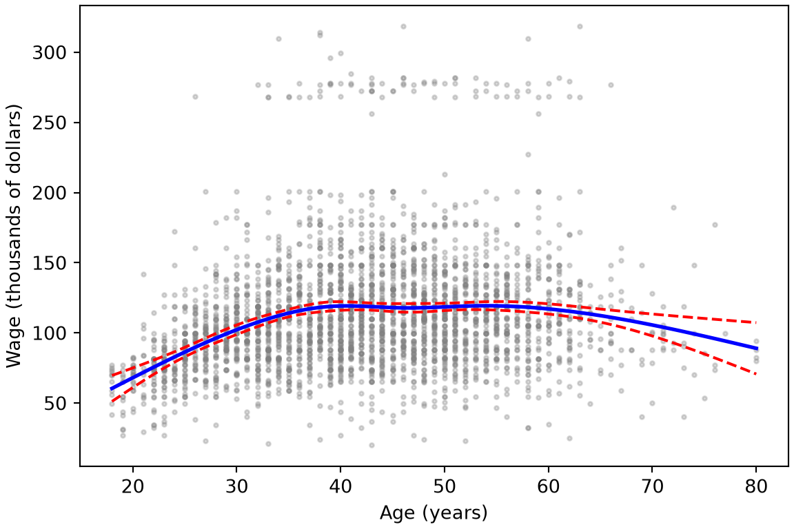
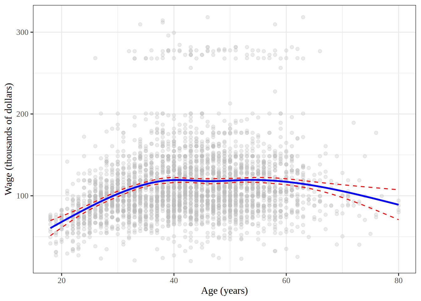
Fit a natural spline of wage on age with df = 5, and plot the fit over the data, with \(95\%\) confidence bands.

TipHint

In R, splines::ns(age, df = 5) builds the columns inside the formula, and predict() with type = "conf_int" gives the bands. In Python, patsy’s cr() builds a natural cubic spline inside an smf.ols() formula; give it the interior knots that ns() would choose, at the quintiles of age, and get_prediction() gives the bands.

Solution 22.

Show code
import matplotlib.pyplot as plt
import numpy as np

# a natural spline with df = 5 has 4 interior knots, at the quintiles
# of age, as R's ns() places them; cr() is patsy's natural cubic spline
ns_knots = tuple(np.quantile(wage_py["age"], [0.2, 0.4, 0.6, 0.8]))
ns_formula = "wage ~ cr(age, knots=ns_knots, constraints='center')"
M_ns = smf.ols(ns_formula, wage_py).fit()
grid_py = np.linspace(wage_py["age"].min(), wage_py["age"].max(), 100)
age_df = pd.DataFrame({"age": grid_py})
ns_bands = M_ns.get_prediction(age_df).summary_frame(alpha=0.05)

fig, ax = plt.subplots(figsize=(6, 4), layout="constrained")
ax.scatter(wage_py["age"], wage_py["wage"], c="gray", s=5, alpha=0.3);
ax.plot(grid_py, ns_bands["mean"], "b", linewidth=2);
ax.plot(grid_py, ns_bands["mean_ci_lower"], "r--");
ax.plot(grid_py, ns_bands["mean_ci_upper"], "r--");
ax.set_xlabel("Age (years)");
ax.set_ylabel("Wage (thousands of dollars)");
plt.show()
Show code
ns_fit <- linear_reg() |>
  fit(wage ~ splines::ns(age, df = 5), data = wage)
age_range <- range(wage$age)
grid_ages <- seq(age_range[1], age_range[2], length.out = 100)
ns_grid <- tibble(age = grid_ages)
ns_mean <- predict(ns_fit, ns_grid)
ns_band <- predict(ns_fit, ns_grid, type = "conf_int")
ns_curve <- bind_cols(ns_grid, ns_mean, ns_band)
ns_plot <- wage |>
  ggplot() +
  aes(x = age, y = wage) +
  geom_point(colour = "gray", alpha = 0.3) +
  geom_line(aes(y = .pred), ns_curve, colour = "blue", linewidth = 1) +
  geom_line(aes(y = .pred_lower), ns_curve, colour = "red", linetype = 2) +
  geom_line(aes(y = .pred_upper), ns_curve, colour = "red", linetype = 2) +
  labs(x = "Age (years)", y = "Wage (thousands of dollars)")
ns_plot
Figure 7: Wage against age, with a natural cubic spline fit with df = 5, and its \(95\%\) confidence bands.

Figure 7 shows wage rising until about age \(40\), staying level through middle age, and falling after \(60\). The bands are widest at the oldest ages, where there are fewest workers.

5 Smoothing splines

ExrExercise 23 (Lab: predict a wage with a smoothing spline)

Exercise 23 (Lab: predict a wage with a smoothing spline) Fit wage on age with a smoothing spline whose effective degrees of freedom are \(4\), and use it to predict the wage of a \(50\)-year-old.

TipHint

In R, smooth.spline() takes the effective degrees of freedom as df and finds the smoothing parameter itself. In Python, scipy.interpolate.make_smoothing_spline() takes the smoothing parameter instead, and needs each distinct age only once, so pass it the sample mean wage at each age, and the count of workers at each age as w. The effective degrees of freedom are the trace of the smoother matrix, and the smoother matrix times the \(j\)th unit vector is the fit to that unit vector.

Solution 23.

import numpy as np
import pandas as pd
from scipy.interpolate import make_smoothing_spline
from scipy.optimize import brentq

wage_ss_py = pd.read_csv("data/wage.csv")
# make_smoothing_spline needs distinct ages,
# so fit the mean wage at each age, weighted by the number of workers
by_age_py = wage_ss_py.groupby("age")["wage"].agg(["mean", "size"])
ages_py = by_age_py.index.to_numpy(dtype=float)
means_py = by_age_py["mean"].to_numpy()
counts_py = by_age_py["size"].to_numpy(dtype=float)
unit_py = np.eye(len(ages_py))


def smoother_df(lam):
    """Trace of the smoother matrix: the fit to unit vector j, at age j."""
    total = 0.0
    for j, unit_j in enumerate(unit_py):
        fit_j = make_smoothing_spline(ages_py, unit_j, w=counts_py, lam=lam)
        total += fit_j(ages_py[j])
    return total


# search over log10(lambda) for the value that gives 4 degrees of freedom
log_lam_py = brentq(lambda t: smoother_df(10**t) - 4, -2, 10)
lam_py = 10**log_lam_py
smooth_py = make_smoothing_spline(ages_py, means_py, w=counts_py, lam=lam_py)
pred_smooth_py = float(smooth_py(50.0))
pred_smooth_py
119.61199883499343
wage_ss <- readr::read_csv("data/wage.csv", show_col_types = FALSE)
# all.knots = TRUE puts a knot at every distinct age, as the definition does
smooth_fit <- smooth.spline(
  wage_ss$age,
  wage_ss$wage,
  df = 4,
  all.knots = TRUE
)
smooth_pred <- predict(smooth_fit, x = 50)
pred_smooth_r <- smooth_pred$y
pred_smooth_r
[1] 119.6118

Replacing the wages at each age by their sample mean, counted once per worker of that age, leaves the smoothing spline unchanged, because it changes the criterion only by a term that does not depend on the curve. It leaves the trace of the smoother matrix unchanged too, so both code paths solve for the same effective degrees of freedom. By default, smooth.spline() uses fewer knots than distinct ages when there are more than \(49\) of them, so the R code passes all.knots = TRUE.

The predicted wage of a \(50\)-year-old is 119.6 thousand dollars in the R run and 119.6 in the Python run. The two programs scale the smoothing parameter differently, so compare their effective degrees of freedom, not their values of \(\regpar\).

ExrExercise 24 (Lab: fit a smoothing spline with a fixed smoothing parameter)

Exercise 24 (Lab: fit a smoothing spline with a fixed smoothing parameter) Fit wage on age with a smoothing spline whose smoothing parameter \(\regpar\) is \(0.6\). How many effective degrees of freedom does the fit have?

TipHint

In Python, reuse make_smoothing_spline() and smoother_df() from Exercise 23. In R, smooth.spline() rescales age to run from \(0\) to \(1\) before it applies the penalty, so divide \(\regpar\) by the cube of the oldest age minus the youngest to put it on the Python scale.

Solution 24.

Show code
fixed_lam_py = 0.6
fixed_ss_py = make_smoothing_spline(
    ages_py, means_py, w=counts_py, lam=fixed_lam_py
)
df_fixed_py = smoother_df(fixed_lam_py)
df_fixed_py
np.float64(49.994142029011776)
Show code
fixed_lam <- 0.6
age_limits_ss <- range(wage_ss$age)
age_width <- age_limits_ss[2] - age_limits_ss[1]
# smooth.spline() rescales age to [0, 1], which divides lambda by width^3
fixed_fit <- smooth.spline(
  wage_ss$age,
  wage_ss$wage,
  lambda = fixed_lam / age_width^3,
  all.knots = TRUE
)
df_fixed <- fixed_fit$df
df_fixed
[1] 50.00783

On the Python scale, \(\regpar = 0.6\) gives 50 effective degrees of freedom in the R run and 50 in the Python run. There are 61 distinct ages, so this penalty is small, and the fit is wigglier than the \(4\)-degree-of-freedom fit of Exercise 23.

A smoothing spline is a generalized additive model with one feature and squared-error loss. The book fits this one with LinearGAM(s(0, lam=0.6)) from the pygam package [1, Sec. 7.8]. pygam scales the penalty differently, and it puts fewer knots on age, so the same \(\regpar\) gives a smoother fit there. Compare fits from different programs by their effective degrees of freedom, not by their values of \(\regpar\).

ExrExercise 25 (Lab: vary the smoothing parameter)

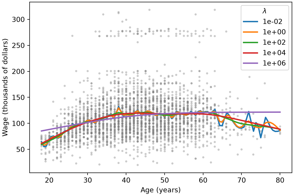
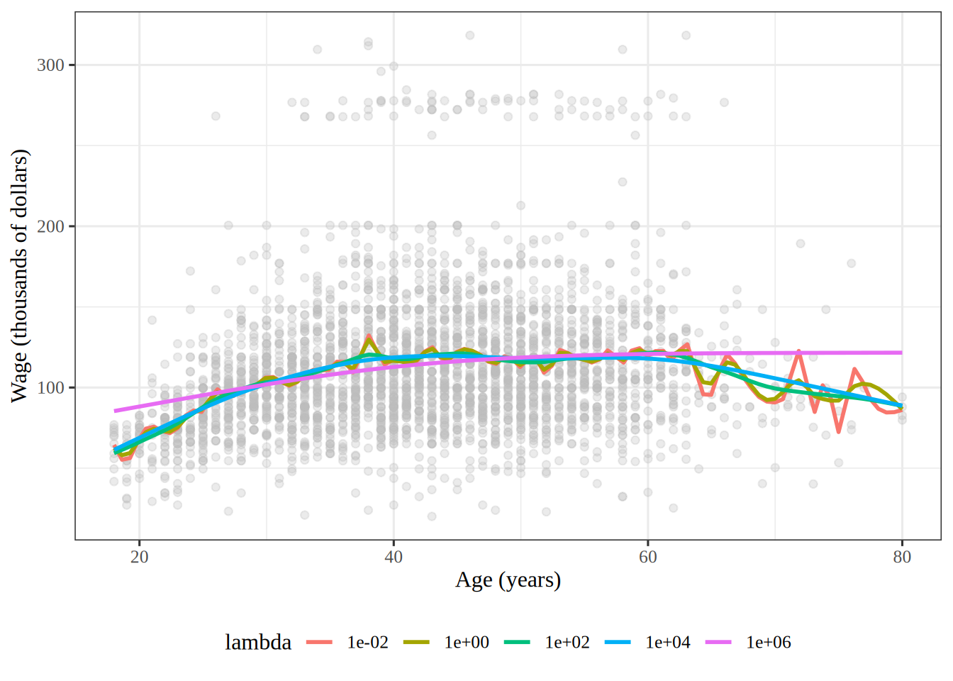
Exercise 25 (Lab: vary the smoothing parameter) A smoothing spline’s smoothing parameter \(\regpar\) trades closeness to the data against roughness. Fit a smoothing spline of wage on age in the Wage data for each \(\regpar\) in \(10^{-2}\), \(10^{0}\), \(10^{2}\), \(10^{4}\) and \(10^{6}\), and plot the fits over the data.

TipHint

In Python, reuse make_smoothing_spline() and the sample mean wage at each age from Exercise 23, and pass each \(\regpar\) as lam. In R, smooth.spline() takes \(\regpar\) as lambda, but it rescales age to run from \(0\) to \(1\) first, so pass \(\regpar / r^3\), where \(r\) is the largest age minus the smallest, to get the same fit.

Solution 25.

Show code
import matplotlib.pyplot as plt

grid_ss_py = np.linspace(ages_py.min(), ages_py.max(), 100)
lams_py = np.logspace(-2, 6, 5)
# the fit for each lambda, evaluated on the grid
lam_curves_py = {}
for lam in lams_py:
    fit_lam = make_smoothing_spline(ages_py, means_py, w=counts_py, lam=lam)
    lam_curves_py[lam] = fit_lam(grid_ss_py)
lam_dfs_py = [smoother_df(lam) for lam in lams_py]

fig, ax = plt.subplots(figsize=(6, 4), layout="constrained")
ax.scatter(wage_ss_py["age"], wage_ss_py["wage"], c="gray", s=5, alpha=0.3);
for lam, curve in lam_curves_py.items():
    ax.plot(grid_ss_py, curve, linewidth=2, label=f"{lam:.0e}");
ax.set_xlabel("Age (years)");
ax.set_ylabel("Wage (thousands of dollars)");
ax.legend(title=r"$\lambda$");
plt.show()
Show code
lams <- 10^seq(-2, 6, by = 2)
lam_labels <- format(lams, scientific = TRUE)
age_range <- range(wage_ss$age)
age_span <- diff(age_range)
grid_ss <- seq(age_range[1], age_range[2], length.out = 100)

# smooth.spline() rescales age to [0, 1],
# which divides the penalty by the cube of the age range
lambda_curves <- lams |>
  purrr::map(\(lam) {
    lam_fit <- smooth.spline(
      wage_ss$age,
      wage_ss$wage,
      lambda = lam / age_span^3,
      all.knots = TRUE
    )
    lam_grid <- predict(lam_fit, x = grid_ss)
    tibble(age = grid_ss, wage = lam_grid$y, lambda = lam, df = lam_fit$df)
  }) |>
  purrr::list_rbind() |>
  mutate(lambda = factor(lambda, levels = lams, labels = lam_labels))
lambda_dfs <- lambda_curves |>
  distinct(lambda, df)
lambda_plot <- wage_ss |>
  ggplot() +
  aes(x = age, y = wage) +
  geom_point(colour = "gray", alpha = 0.3) +
  geom_line(aes(colour = lambda), lambda_curves, linewidth = 1) +
  labs(x = "Age (years)", y = "Wage (thousands of dollars)", colour = "lambda")
lambda_plot
Figure 8: Wage against age, with smoothing spline fits for five values of the smoothing parameter.

In Figure 8, the effective degrees of freedom fall from 60.5 at \(\regpar = 10^{-2}\) to 2.5 at \(\regpar = 10^{6}\), in both tabs. The fits with small \(\regpar\) follow the sample mean wage at each age, and wiggle past age \(65\), where few workers are. The fit with \(\regpar = 10^{6}\) is close to a straight line, and misses the rise in wage through the twenties.

ExrExercise 26 (Lab: choose the smoothing parameter by generalized cross-validation)

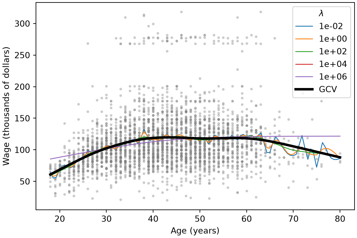
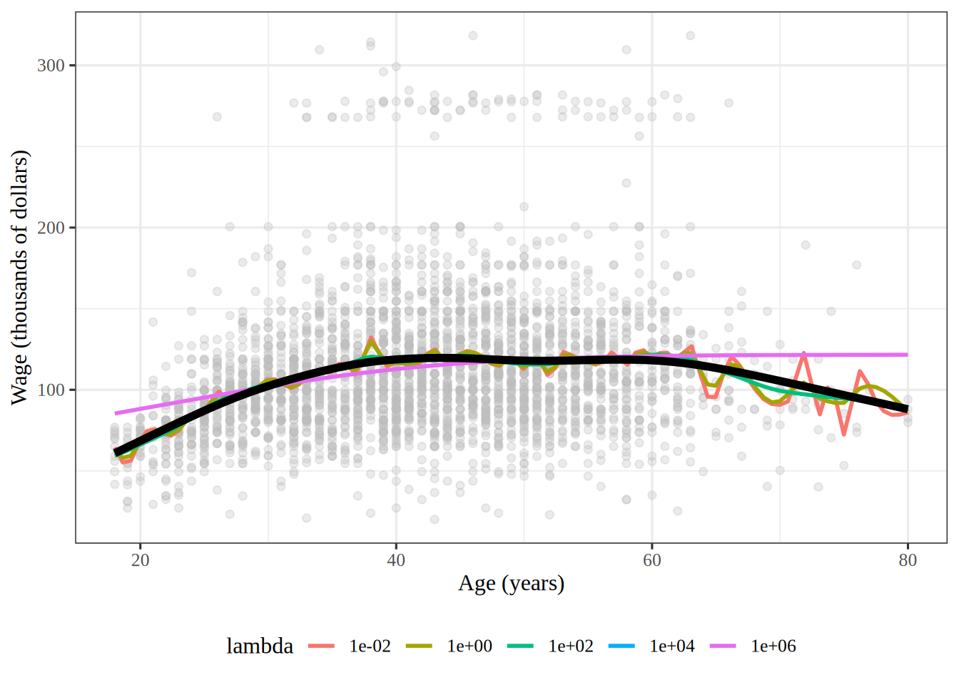
Exercise 26 (Lab: choose the smoothing parameter by generalized cross-validation) Instead of fixing the smoothing parameter \(\regpar\), choose it by minimizing the generalized cross-validation score of the fit of wage on age, and add that fit to the plot of Exercise 25.

TipHint

In R, smooth.spline() minimizes generalized cross-validation when it is given neither df nor lambda. In Python, make_smoothing_spline() with no lam scores its own data, which here are the sample means at each age rather than the workers, so compute the score over all \(n\) workers, \(n \cdot \RSS / \devof{n}{\trf{S_\regpar}}^2\), with smoother_df() from Exercise 23 for the trace, and minimize it over \(\log_{10} \regpar\).

Solution 26.

Show code
from scipy.optimize import minimize_scalar

ages_all_py = wage_ss_py["age"].to_numpy(dtype=float)
wages_all_py = wage_ss_py["wage"].to_numpy()
n_ss_py = len(wages_all_py)


def gcv_score(log_lam):
    """Generalized cross-validation over all workers: n RSS / (n - df)^2."""
    lam = 10**log_lam
    fit = make_smoothing_spline(ages_py, means_py, w=counts_py, lam=lam)
    rss = np.sum((wages_all_py - fit(ages_all_py)) ** 2)
    return n_ss_py * rss / (n_ss_py - smoother_df(lam)) ** 2


# search a grid of log10(lambda), then refine around the best grid point
log_grid_py = np.linspace(-2, 6, 33)
gcv_grid_py = [gcv_score(t) for t in log_grid_py]
best_log_py = log_grid_py[np.argmin(gcv_grid_py)]
gcv_opt_py = minimize_scalar(
    gcv_score, bounds=(best_log_py - 0.25, best_log_py + 0.25), method="bounded"
)
lam_gcv_py = 10**gcv_opt_py.x
df_gcv_py = smoother_df(lam_gcv_py)
fit_gcv_py = make_smoothing_spline(ages_py, means_py, w=counts_py, lam=lam_gcv_py)

fig, ax = plt.subplots(figsize=(6, 4), layout="constrained")
ax.scatter(wage_ss_py["age"], wage_ss_py["wage"], c="gray", s=5, alpha=0.3);
for lam, curve in lam_curves_py.items():
    ax.plot(grid_ss_py, curve, linewidth=1, label=f"{lam:.0e}");
ax.plot(grid_ss_py, fit_gcv_py(grid_ss_py), "k", linewidth=3, label="GCV");
ax.set_xlabel("Age (years)");
ax.set_ylabel("Wage (thousands of dollars)");
ax.legend(title=r"$\lambda$");
plt.show()
Show code
# with neither df nor lambda, smooth.spline() minimizes
# generalized cross-validation
gcv_fit <- smooth.spline(wage_ss$age, wage_ss$wage, all.knots = TRUE)
lam_gcv <- gcv_fit$lambda * age_span^3
log_lam_gcv <- log10(lam_gcv)
df_gcv <- gcv_fit$df
gcv_grid <- predict(gcv_fit, x = grid_ss)
gcv_curve <- tibble(age = grid_ss, wage = gcv_grid$y)
gcv_plot <- lambda_plot +
  geom_line(data = gcv_curve, colour = "black", linewidth = 2)
gcv_plot
Figure 9: The fits of Figure 8, with the fit whose smoothing parameter minimizes generalized cross-validation in black.

On the Python scale, generalized cross-validation chooses \(\regpar\) = 8310 in the R run and 8310 in the Python run. The two fits have 6.47 and 6.47 effective degrees of freedom. The base-10 logarithm of that \(\regpar\) is 3.9, between the \(10^{2}\) and \(10^{4}\) of Figure 8, so in Figure 9 its fit is smoother than the curves that wiggle past age \(65\), but still rises through the twenties and falls after \(60\).

ExrExercise 27 (Lab: set how flexible a smoothing spline is)

Exercise 27 (Lab: set how flexible a smoothing spline is) Plot, over the data, the smoothing spline fits of wage on age with \(1\), \(3\), \(4\), \(8\) and \(15\) effective degrees of freedom besides the intercept.

TipHint

A smoothing spline’s effective degrees of freedom count the intercept, so solve for the smoothing parameter that gives one more than each number, with brentq() and smoother_df() as in Exercise 23, or with df in smooth.spline(). One besides the intercept needs an infinite smoothing parameter.

Solution 27.

Show code
df_targets = [1, 3, 4, 8, 15]
fig, ax = plt.subplots(figsize=(6, 4), layout="constrained")
ax.scatter(wage_ss_py["age"], wage_ss_py["wage"], c="gray", s=5, alpha=0.3);
for df in df_targets:
    if df == 1:
        # an infinite lambda leaves only the least squares line
        line = np.polyfit(ages_all_py, wages_all_py, 1)
        curve = np.polyval(line, grid_ss_py)
    else:
        # df counts the age term; the intercept adds 1
        log_lam = brentq(lambda t: smoother_df(10**t) - (df + 1), -2, 10)
        fit_df = make_smoothing_spline(ages_py, means_py, w=counts_py, lam=10**log_lam)
        curve = fit_df(grid_ss_py)
    ax.plot(grid_ss_py, curve, linewidth=2, label=f"{df}");
ax.set_xlabel("Age (years)");
ax.set_ylabel("Wage (thousands of dollars)");
ax.legend(title="Degrees of freedom");
plt.show()
Show code
df_targets <- c(1, 3, 4, 8, 15)

grid_ages <- tibble(age = grid_ss)
df_curves <- df_targets |>
  purrr::map(\(df) {
    is_line <- df == 1
    if (is_line) {
      # an infinite lambda leaves only the least squares line
      line_fit <- lm(wage ~ age, data = wage_ss)
      grid_wage <- predict(line_fit, grid_ages)
    } else {
      # df counts the age term; the intercept adds 1
      df_fit <- smooth.spline(
        wage_ss$age,
        wage_ss$wage,
        df = df + 1,
        all.knots = TRUE
      )
      df_grid <- predict(df_fit, x = grid_ss)
      grid_wage <- df_grid$y
    }
    mutate(grid_ages, wage = grid_wage, df = df)
  }) |>
  purrr::list_rbind() |>
  mutate(df = factor(df, levels = df_targets))
df_plot <- wage_ss |>
  ggplot() +
  aes(x = age, y = wage) +
  geom_point(colour = "gray", alpha = 0.3) +
  geom_line(aes(colour = df), df_curves, linewidth = 1) +
  labs(
    x = "Age (years)",
    y = "Wage (thousands of dollars)",
    colour = "Degrees of freedom"
  )
df_plot
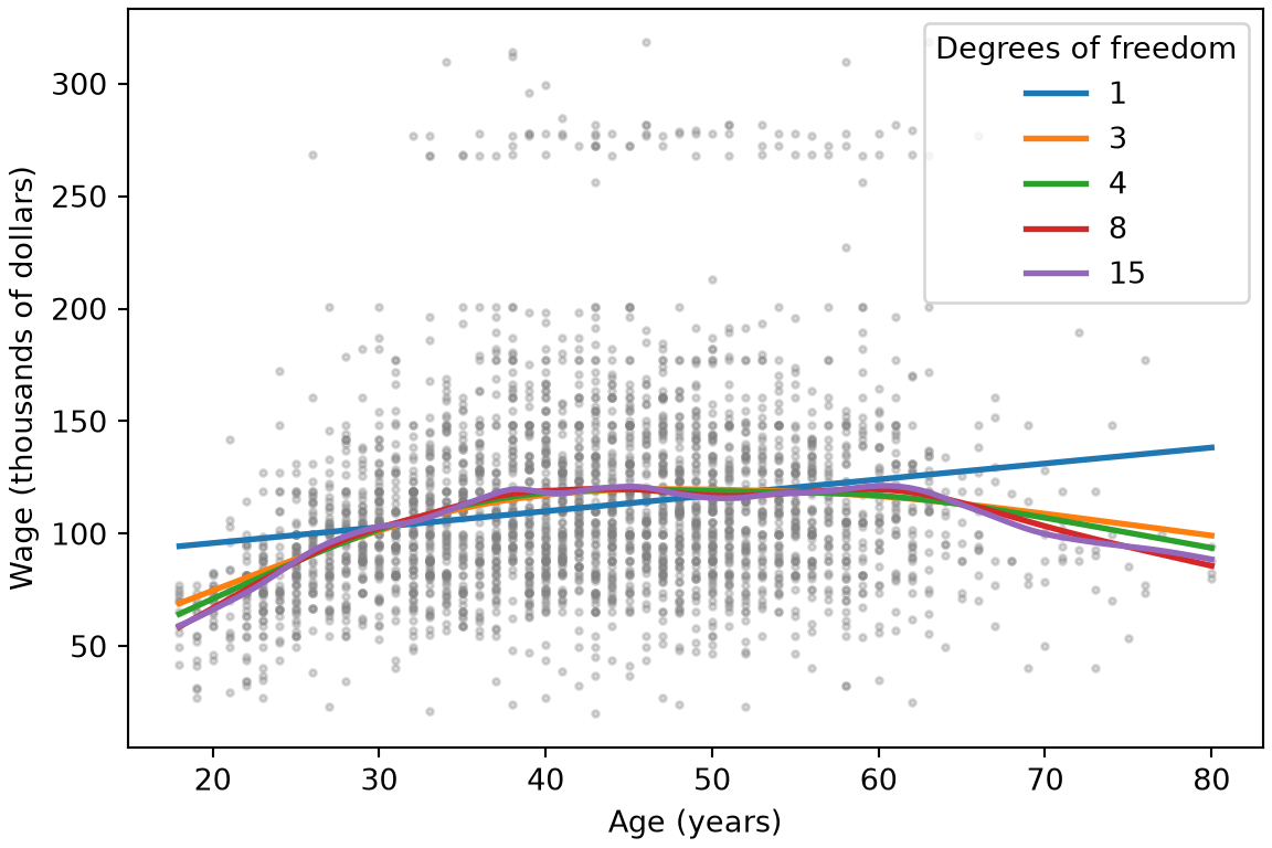
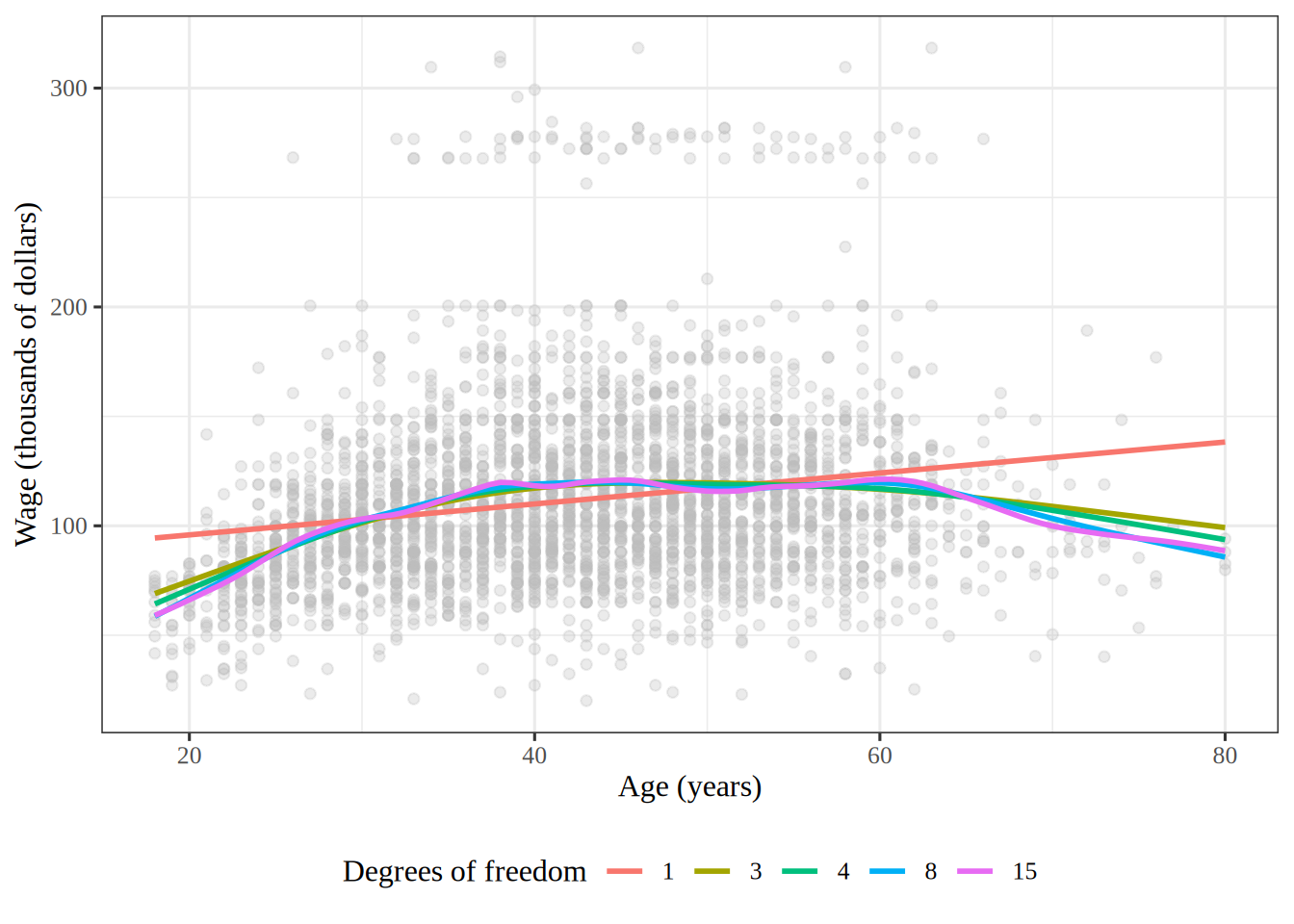
Figure 10: Wage against age, with smoothing spline fits for five numbers of effective degrees of freedom besides the intercept.

In Figure 10, \(1\) effective degree of freedom besides the intercept gives the least squares line. That line keeps rising after age \(60\), where the wages fall. With \(3\) or more, the fits rise until about age \(40\), level off, and fall after \(60\). Each added one lets the fit bend more.

6 Local regression

ExrExercise 28 (Lab: compare two spans for local regression)

Exercise 28 (Lab: compare two spans for local regression) A LOESS curve fits a line near each age, using only the share of workers nearest that age, so its span decides how smooth the curve is, as the smoothing parameter does for a smoothing spline.

Plot LOESS curves of wage on age with spans of \(0.2\) and \(0.5\) over the data. How does the smaller span change the curve?

TipHint

In Python, statsmodels.nonparametric.lowess() takes the span as frac, the ages at which to evaluate the curve as xvals, and it=0 to skip its robustness passes. In R, loess() takes the span as span; pass degree = 1 for a local linear fit and surface = "direct" to fit at each age rather than interpolate.

Solution 28.

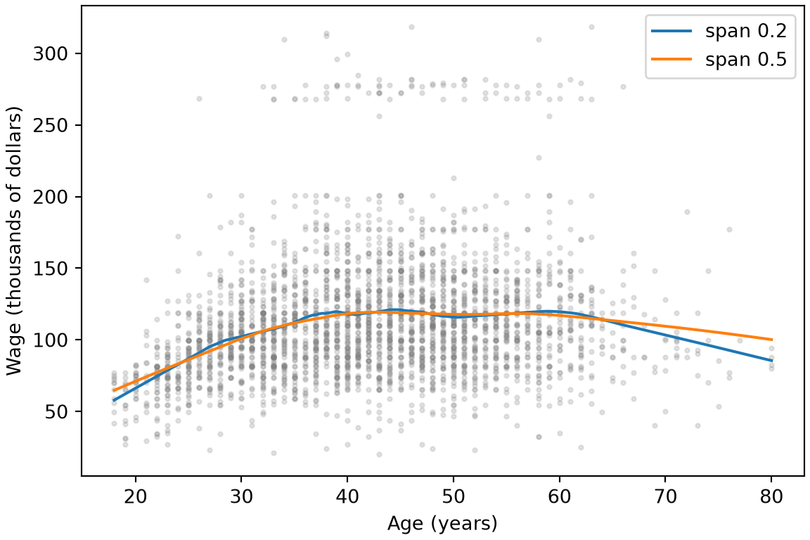
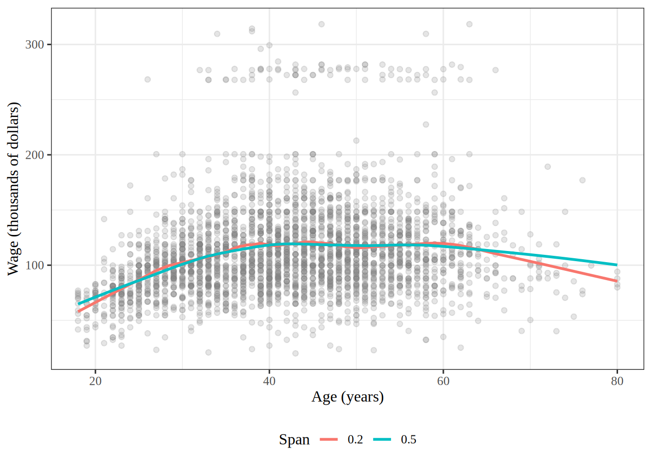
Figure 11: Wage against age, with LOESS curves for spans of \(0.2\) and \(0.5\).
import matplotlib.pyplot as plt
import numpy as np
import pandas as pd
import statsmodels.api as sm

wage_lo_py = pd.read_csv("data/wage.csv")
# evaluate each curve on a fine grid of ages, so the plot is smooth
age_grid_py = np.linspace(18, 80, 200)
fig, ax = plt.subplots(figsize=(6, 4), layout="constrained")
ax.scatter(wage_lo_py["age"], wage_lo_py["wage"], s=5, alpha=0.2, color="gray");
for span in (0.2, 0.5):
    # it=0 skips the robustness passes, so this is plain local linear regression
    curve = sm.nonparametric.lowess(
        wage_lo_py["wage"], wage_lo_py["age"], frac=span, it=0, xvals=age_grid_py
    )
    ax.plot(age_grid_py, curve, label=f"span {span}");
ax.set_xlabel("Age (years)");
ax.set_ylabel("Wage (thousands of dollars)");
ax.legend();
plt.show()

Scatterplot of wage against age for 3000 workers, with two LOESS curves. Both rise through the twenties and thirties, level off in middle age and fall after about 60. The span 0.2 curve has small bends between ages 40 and 60 and falls more steeply past age 65 than the span 0.5 curve.

wage_lo <- readr::read_csv("data/wage.csv", show_col_types = FALSE)
# evaluate each curve on a fine grid of ages, so the plot is smooth
ages <- seq(18, 80, length.out = 200)
age_grid <- tibble(age = ages)
# degree = 1 fits a local line; surface = "direct" fits at every grid age
loess_narrow <- loess(
  wage ~ age,
  data = wage_lo,
  span = 0.2,
  degree = 1,
  surface = "direct"
)
loess_wide <- loess(
  wage ~ age,
  data = wage_lo,
  span = 0.5,
  degree = 1,
  surface = "direct"
)
wage_narrow <- predict(loess_narrow, age_grid)
wage_wide <- predict(loess_wide, age_grid)
curve_narrow <- mutate(age_grid, span = "0.2", wage = wage_narrow)
curve_wide <- mutate(age_grid, span = "0.5", wage = wage_wide)
curves <- bind_rows(curve_narrow, curve_wide)
wage_lo |>
  ggplot() +
  aes(x = age, y = wage) +
  geom_point(alpha = 0.2, color = "gray50") +
  geom_line(data = curves, aes(color = span), linewidth = 1) +
  labs(x = "Age (years)", y = "Wage (thousands of dollars)", color = "Span")

Scatterplot of wage against age for 3000 workers, with two LOESS curves. Both rise through the twenties and thirties, level off in middle age and fall after about 60. The span 0.2 curve has small bends between ages 40 and 60 and falls more steeply past age 65 than the span 0.5 curve.

In Figure 11, the curve with span \(0.2\) fits each line to fewer neighbors, so it follows the data more closely than the curve with span \(0.5\). It has small bends between ages \(40\) and \(60\), and past age \(65\), where few workers are, it falls more steeply. The smaller span trades a lower bias for a higher variance.

7 Additive models

ExrExercise 29 (Lab: predict a wage with an additive model)

Exercise 29 (Lab: predict a wage with an additive model) Fit an additive model of wage with three terms: a cubic regression spline of year whose interior knots are at the median, a cubic regression spline of age with interior knots at the terciles, and education as a categorical variable. Use it to predict the wage of a \(50\)-year-old who graduated from college, in \(2006\).

TipHint

The bs function builds a spline basis for each of the first two terms inside a formula, and a column of text is treated as a category automatically. In R, splines::bs() builds the spline columns, with other default settings.

Solution 29.

import pandas as pd
from sklearn.compose import make_column_transformer
from sklearn.linear_model import LinearRegression
from sklearn.pipeline import make_pipeline
from sklearn.preprocessing import OneHotEncoder, SplineTransformer

wage_add_py = pd.read_csv("data/wage.csv")
year_basis_py = SplineTransformer(n_knots=3, knots="quantile")
age_basis_py = SplineTransformer(n_knots=4, knots="quantile")
terms_py = make_column_transformer(
    (year_basis_py, ["year"]),
    (age_basis_py, ["age"]),
    (OneHotEncoder(drop="first"), ["education"]),
)
additive_py = make_pipeline(terms_py, LinearRegression())
additive_py.fit(wage_add_py.drop(columns="wage"), wage_add_py["wage"])
Pipeline(steps=[('columntransformer',
                 ColumnTransformer(transformers=[('splinetransformer-1',
                                                  SplineTransformer(knots='quantile',
                                                                    n_knots=3),
                                                  ['year']),
                                                 ('splinetransformer-2',
                                                  SplineTransformer(knots='quantile',
                                                                    n_knots=4),
                                                  ['age']),
                                                 ('onehotencoder',
                                                  OneHotEncoder(drop='first'),
                                                  ['education'])])),
                ('linearregression', LinearRegression())])
In a Jupyter environment, please rerun this cell to show the HTML representation or trust the notebook.
On GitHub, the HTML representation is unable to render, please try loading this page with nbviewer.org.
worker_py = pd.DataFrame(
    {"year": [2006], "age": [50], "education": ["4. College Grad"]}
)
pred_additive_py = additive_py.predict(worker_py)[0]
pred_additive_py
np.float64(131.2436523995633)
wage_add <- readr::read_csv("data/wage.csv", show_col_types = FALSE)
additive_formula <- wage ~ splines::bs(year, df = 4) +
  splines::bs(age, df = 5) +
  education
additive_fit <- linear_reg() |>
  fit(additive_formula, data = wage_add)
worker <- tibble(year = 2006, age = 50, education = "4. College Grad")
additive_pred <- predict(additive_fit, new_data = worker)
pred_additive_r <- additive_pred$.pred
pred_additive_r
[1] 131.2437

The two code paths specify the same terms. In R, df = 4 gives one interior knot, at the median of year, and df = 5 gives two, at the terciles of age. In Python, n_knots = 3 and n_knots = 4 count the two boundary points as well, so they give the same interior placements.

The predicted wage is 131.2 thousand dollars in the R run and 131.2 in the Python run.

ExrExercise 30 (Lab: build an additive model by hand)

Exercise 30 (Lab: build an additive model by hand) Exercise 29 fit an additive model of wage through a formula. Build one by hand instead: stack a natural spline basis for age with df = 4, a natural spline basis for year with df = 5, and an indicator column for each level of education into one model matrix, and fit wage on it by least squares with no separate intercept. How many columns does it have?

TipHint

In Python, patsy’s cr() inside dmatrix() builds natural spline columns; give it the interior knots that R’s ns() would choose, at the sample quantiles \(0.25\), \(0.5\) and \(0.75\) of age and \(0.2\), \(0.4\), \(0.6\) and \(0.8\) of year. pd.get_dummies() builds the indicator columns, and np.hstack() stacks the pieces. In R, splines::ns(), model.matrix(~ education - 1) and cbind() do the same.

Solution 30.

Show code
import numpy as np
import pandas as pd
import statsmodels.api as sm
from patsy import dmatrix

wage_bh_py = pd.read_csv("data/wage.csv")
# cr() is patsy's natural cubic spline; df = 4 and df = 5 mean 3 and 4
# interior knots, at the quartiles and quintiles, as R's ns() places them
age_knots_bh = tuple(np.quantile(wage_bh_py["age"], [0.25, 0.5, 0.75]))
year_knots_bh = tuple(np.quantile(wage_bh_py["year"], [0.2, 0.4, 0.6, 0.8]))
ns_age_bh = dmatrix("cr(age, knots=age_knots_bh, constraints='center') - 1", wage_bh_py)
ns_year_bh = dmatrix("cr(year, knots=year_knots_bh, constraints='center') - 1", wage_bh_py)
# one indicator column per level of education, and no intercept
edu_bh = pd.get_dummies(wage_bh_py["education"], dtype=float)
X_bh = np.hstack([ns_age_bh, ns_year_bh, edu_bh])
gam_bh = sm.OLS(wage_bh_py["wage"], X_bh).fit()
X_bh.shape
(3000, 14)
Show code
wage_bh <- readr::read_csv("data/wage.csv", show_col_types = FALSE)
ns_age <- splines::ns(wage_bh$age, df = 4)
ns_year <- splines::ns(wage_bh$year, df = 5)
# one indicator column per level of education, and no intercept
edu_bh <- model.matrix(~ education - 1, data = wage_bh)
x_bh <- cbind(ns_age, ns_year, edu_bh) # nolint: undesirable_function_linter
gam_bh <- lm(wage_bh$wage ~ x_bh - 1)
dim(x_bh)
[1] 3000   14

Both tabs’ model matrices have 14 columns: 4 for age, 5 for year and one for each of the 5 levels of education. The indicator columns for education add up to a vector of ones, so they play the part of the intercept, and the model has no separate one.

ExrExercise 31 (Lab: plot the partial dependence on age)

Exercise 31 (Lab: plot the partial dependence on age) Plot the age term of the additive model of Exercise 30, with \(95\%\) confidence bands: predict on a matrix whose columns all sit at their means, except the age columns, which run over a grid of \(100\) ages, and shift the curve and its bands down by the curve’s mean.

TipHint

In Python, build_design_matrices() with the age columns’ design_info evaluates them on the grid, and the fit’s get_prediction() gives the bands. In R, predict() on an ns() basis evaluates it at new ages, and the standard error of each prediction \(\dprod{\vx}{\hat{\vbeta}}\) is \(\sqrt{\qform{V}{\vx}}\), where \(V\) is the fit’s vcov().

Solution 31.

Show code
import matplotlib.pyplot as plt
from patsy import build_design_matrices

age_grid_bh = np.linspace(wage_bh_py["age"].min(), wage_bh_py["age"].max(), 100)
# every column at its mean, then the age columns swept across the grid
X_age_bh = np.tile(X_bh.mean(axis=0), (100, 1))
age_cols_bh = build_design_matrices([ns_age_bh.design_info], {"age": age_grid_bh})
X_age_bh[:, :4] = age_cols_bh[0]
age_pred_bh = gam_bh.get_prediction(X_age_bh)
age_bounds_bh = age_pred_bh.conf_int(alpha=0.05)
center_age_bh = age_pred_bh.predicted_mean.mean()
partial_age_bh = age_pred_bh.predicted_mean - center_age_bh
age_bounds_bh = age_bounds_bh - center_age_bh

fig, ax = plt.subplots(figsize=(6, 4), layout="constrained")
ax.plot(age_grid_bh, partial_age_bh, "b", linewidth=2);
ax.plot(age_grid_bh, age_bounds_bh, "r--");
ax.set_xlabel("Age (years)");
ax.set_ylabel("Effect on wage (thousands of dollars)");
plt.show()
Show code
age_range_bh <- range(wage_bh$age)
age_grid_bh <- seq(age_range_bh[1], age_range_bh[2], length.out = 100)
# every column at its mean, then the age columns swept across the grid
x_means <- colMeans(x_bh)
n_cols <- length(x_means)
x_age <- matrix(x_means, nrow = 100, ncol = n_cols, byrow = TRUE)
x_age[, 1:4] <- predict(ns_age, age_grid_bh)
beta_bh <- coef(gam_bh)
vcov_bh <- vcov(gam_bh)
t_crit <- qt(0.975, df = gam_bh$df.residual)
age_fit <- (x_age %*% beta_bh)[, 1]
age_cov <- x_age %*% vcov_bh
age_var <- rowSums(age_cov * x_age)
age_se <- sqrt(age_var)
center_age <- mean(age_fit)
partial_age <- tibble(
  age = age_grid_bh,
  effect = age_fit - center_age,
  lower = effect - t_crit * age_se,
  upper = effect + t_crit * age_se
)
peak_age <- partial_age |>
  slice_max(effect) |>
  pull(age)
partial_age |>
  ggplot() +
  aes(x = age, y = effect) +
  geom_line(colour = "blue", linewidth = 1) +
  geom_line(aes(y = lower), colour = "red", linetype = 2) +
  geom_line(aes(y = upper), colour = "red", linetype = 2) +
  labs(x = "Age (years)", y = "Effect on wage (thousands of dollars)")
Figure 12: The partial dependence of wage on age in the additive model, with \(95\%\) confidence bands.

Holding every other column at its mean holds the year and education terms at their means, so the curve in Figure 12 is the age component function plus a constant, and the shift removes the constant. Wage rises steeply until about age 45 and then falls slowly, with the confidence bands widest at the oldest ages, where there are fewest workers.

ExrExercise 32 (Lab: plot the partial dependence on year)

Exercise 32 (Lab: plot the partial dependence on year) Plot the year term of the additive model of Exercise 30 in the same way as the age term in Exercise 31, over a grid of \(100\) years.

Solution 32.

Show code
year_grid_bh = np.linspace(wage_bh_py["year"].min(), wage_bh_py["year"].max(), 100)
# every column at its mean, then the year columns swept across the grid
X_year_bh = np.tile(X_bh.mean(axis=0), (100, 1))
year_cols_bh = build_design_matrices([ns_year_bh.design_info], {"year": year_grid_bh})
X_year_bh[:, 4:9] = year_cols_bh[0]
year_pred_bh = gam_bh.get_prediction(X_year_bh)
year_bounds_bh = year_pred_bh.conf_int(alpha=0.05)
center_year_bh = year_pred_bh.predicted_mean.mean()
partial_year_bh = year_pred_bh.predicted_mean - center_year_bh
year_bounds_bh = year_bounds_bh - center_year_bh

fig, ax = plt.subplots(figsize=(6, 4), layout="constrained")
ax.plot(year_grid_bh, partial_year_bh, "b", linewidth=2);
ax.plot(year_grid_bh, year_bounds_bh, "r--");
ax.set_xlabel("Year");
ax.set_ylabel("Effect on wage (thousands of dollars)");
plt.show()
Show code
year_range_bh <- range(wage_bh$year)
year_grid_bh <- seq(year_range_bh[1], year_range_bh[2], length.out = 100)
# every column at its mean, then the year columns swept across the grid
x_year <- matrix(x_means, nrow = 100, ncol = n_cols, byrow = TRUE)
x_year[, 5:9] <- predict(ns_year, year_grid_bh)
year_fit <- (x_year %*% beta_bh)[, 1]
year_cov <- x_year %*% vcov_bh
year_var <- rowSums(year_cov * x_year)
year_se <- sqrt(year_var)
center_year <- mean(year_fit)
partial_year <- tibble(
  year = year_grid_bh,
  effect = year_fit - center_year,
  lower = effect - t_crit * year_se,
  upper = effect + t_crit * year_se
)
year_rise <- partial_year$effect[[100]] - partial_year$effect[[1]]
partial_year |>
  ggplot() +
  aes(x = year, y = effect) +
  geom_line(colour = "blue", linewidth = 1) +
  geom_line(aes(y = lower), colour = "red", linetype = 2) +
  geom_line(aes(y = upper), colour = "red", linetype = 2) +
  labs(x = "Year", y = "Effect on wage (thousands of dollars)")
Figure 13: The partial dependence of wage on year in the additive model, with \(95\%\) confidence bands.

With age and education held fixed, the year term in Figure 13 rises by 8.1 thousand dollars from 2003 to 2009. The dip around 2008 is smaller than the gap between the confidence bands, so the data give no clear sign that wages fell that year.

ExrExercise 33 (Lab: plot the age curve of an additive model with smoothing splines)

Exercise 33 (Lab: plot the age curve of an additive model with smoothing splines) Plot the age component function against age for an additive model of wage that has a smoothing spline in age, another in year, and education as a category.

TipHint

In Python, pygam takes a numeric matrix, so code education by its level numbers with .cat.codes, and build LinearGAM(s(0) + s(1, n_splines=7) + f(2, lam=0)). Here f() marks a categorical feature, and year takes only 7 values, so its spline gets 7 basis functions. partial_dependence(term=0, X=..., width=0.95) returns the age curve and its \(95\%\) bands. In R, mgcv::gam() fits wage ~ s(age, bs = "cr") + s(year, bs = "cr", k = 7) + education, and predict(..., type = "terms", se.fit = TRUE) returns each term’s curve and the numbers to build its bands from.

Solution 33.

Show code
import numpy as np
import pandas as pd
import matplotlib.pyplot as plt
from pygam import LinearGAM, s as s_gam, f as f_gam

wage_gam_py = pd.read_csv("data/wage.csv")
# pygam takes a numeric matrix, so education becomes its level codes
edu_gam_py = wage_gam_py["education"].astype("category")
Xgam = np.column_stack(
    [wage_gam_py["age"], wage_gam_py["year"], edu_gam_py.cat.codes]
)
y_gam = wage_gam_py["wage"].to_numpy()
gam_full = LinearGAM(s_gam(0) + s_gam(1, n_splines=7) + f_gam(2, lam=0))
gam_full = gam_full.fit(Xgam, y_gam)
edof_py = gam_full.statistics_["edof_per_coef"]
edof_age_default_py = edof_py[gam_full.terms.get_coef_indices(0)].sum()

grid_age = gam_full.generate_X_grid(term=0)
pdep_age, band_age = gam_full.partial_dependence(term=0, X=grid_age, width=0.95)
fig, ax = plt.subplots(figsize=(6, 4), layout="constrained")
ax.plot(grid_age[:, 0], pdep_age, "b", linewidth=2);
ax.plot(grid_age[:, 0], band_age, "r--");
ax.set_xlabel("Age (years)");
ax.set_ylabel("Effect on wage (thousands of dollars)");
plt.show()
Show code
wage_gam <- readr::read_csv("data/wage.csv", show_col_types = FALSE)
gam_default <- mgcv::gam(
  wage ~ s(age, bs = "cr") + s(year, bs = "cr", k = 7) + education,
  data = wage_gam
)
gam_default_summary <- summary(gam_default)
edf_age_default <- gam_default_summary$edf[1]

age_range_gam <- range(wage_gam$age)
year_range_gam <- range(wage_gam$year)
age_seq <- seq(age_range_gam[1], age_range_gam[2], length.out = 100)
year_seq <- seq(year_range_gam[1], year_range_gam[2], length.out = 100)
# one grid sweeps age and year together; each term's curve is read separately
gam_grid <- tibble(
  age = age_seq,
  year = year_seq,
  education = wage_gam$education[1]
)
z_crit <- qnorm(0.975)
default_terms <- predict(gam_default, gam_grid, type = "terms", se.fit = TRUE)
partial_age_gam <- gam_grid |>
  mutate(
    effect = default_terms$fit[, "s(age)"],
    lower = effect - z_crit * default_terms$se.fit[, "s(age)"],
    upper = effect + z_crit * default_terms$se.fit[, "s(age)"]
  )
partial_age_gam |>
  ggplot() +
  aes(x = age, y = effect) +
  geom_line(colour = "blue", linewidth = 1) +
  geom_line(aes(y = lower), colour = "red", linetype = 2) +
  geom_line(aes(y = upper), colour = "red", linetype = 2) +
  labs(x = "Age (years)", y = "Effect on wage (thousands of dollars)")
Figure 14: The age term of the additive model with smoothing splines, with \(95\%\) confidence bands: pygam with its default penalty (Python), and mgcv with a penalty that the data choose (R).

year takes only \(7\) values, so its smoother gets \(7\) basis functions. Setting lam=0 on the education term leaves its numbers for the levels unpenalized. The default penalty, lam=0.6, gives the age smoother 15.2 effective degrees of freedom, so the Python curve in Figure 14 is wiggly. mgcv::gam() instead chooses each penalty by generalized cross-validation. It gives age 4.9 effective degrees of freedom and year 1.05, close to a straight line, which agrees with the tests of Exercise 36.

ExrExercise 34 (Lab: give each smoother about 4 degrees of freedom)

Exercise 34 (Lab: give each smoother about 4 degrees of freedom) Plot both component functions of the model of Exercise 33 when its age and year smoothers each have about \(4\) effective degrees of freedom.

TipHint

In Python, search for the lam at which a smoother of one variable alone has \(4 + 1\) effective degrees of freedom, the \(1\) being the intercept that LinearGAM adds, and put that lam on the matching term before refitting. In R, s(age, bs = "cr", k = 5, fx = TRUE) is a cubic regression spline with no penalty and exactly \(4\) effective degrees of freedom.

Solution 34.

Show code
from scipy.optimize import brentq


def approx_lam(X, term, df):
    """The lam at which this term, fit alone, has df degrees of freedom."""
    col = X[:, [term.feature]]

    def gap(log_lam):
        one = LinearGAM(s_gam(0, n_splines=term.n_splines, lam=10**log_lam))
        return one.fit(col, y_gam).statistics_["edof"] - df

    return 10 ** brentq(gap, -3, 6)


age_term = gam_full.terms[0]
age_term.lam = [approx_lam(Xgam, age_term, df=4 + 1)]
year_term = gam_full.terms[1]
year_term.lam = [approx_lam(Xgam, year_term, df=4 + 1)]
gam_full = gam_full.fit(Xgam, y_gam)
edof_py = gam_full.statistics_["edof_per_coef"]
edof_age_py = edof_py[gam_full.terms.get_coef_indices(0)].sum()
edof_year_py = edof_py[gam_full.terms.get_coef_indices(1)].sum()

fig, axes = plt.subplots(1, 2, figsize=(8, 4), layout="constrained")
for term_i, ax, label in zip([0, 1], axes, ["Age", "Year"]):
    grid = gam_full.generate_X_grid(term=term_i)
    pdep, band = gam_full.partial_dependence(term=term_i, X=grid, width=0.95)
    ax.plot(grid[:, term_i], pdep, "b", linewidth=2);
    ax.plot(grid[:, term_i], band, "r--");
    ax.set_xlabel(label);
axes[0].set_ylabel("Effect on wage (thousands of dollars)");
plt.show()
Show code
# k = 5 with fx = TRUE: an unpenalized cubic spline with 4 degrees of freedom
gam_df4 <- mgcv::gam(
  wage ~ s(age, bs = "cr", k = 5, fx = TRUE) +
    s(year, bs = "cr", k = 5, fx = TRUE) +
    education,
  data = wage_gam
)
df4_terms <- predict(gam_df4, gam_grid, type = "terms", se.fit = TRUE)
age_df4 <- tibble(
  term = "Age",
  x = gam_grid$age,
  effect = df4_terms$fit[, "s(age)"],
  se = df4_terms$se.fit[, "s(age)"]
)
year_df4 <- tibble(
  term = "Year",
  x = gam_grid$year,
  effect = df4_terms$fit[, "s(year)"],
  se = df4_terms$se.fit[, "s(year)"]
)
partial_df4 <- bind_rows(age_df4, year_df4) |>
  mutate(lower = effect - z_crit * se, upper = effect + z_crit * se)
partial_df4 |>
  ggplot() +
  aes(x = x, y = effect) +
  geom_line(colour = "blue", linewidth = 1) +
  geom_line(aes(y = lower), colour = "red", linetype = 2) +
  geom_line(aes(y = upper), colour = "red", linetype = 2) +
  facet_wrap(~term, scales = "free_x") +
  labs(x = NULL, y = "Effect on wage (thousands of dollars)")
Figure 15: The age and year terms when each smoother has about \(4\) effective degrees of freedom.

age_term is the term object inside gam_full, not a copy, so setting age_term.lam changes gam_full.terms[0] in place. After the refit, the Python smoothers have 5.1 effective degrees of freedom for age and 4 for year: the search tunes each smoother alone, so with all three terms fit together the counts come out near \(4\) rather than at it. The R smoothers have exactly \(4\) each, because they carry no penalty. pygam does not center a term’s curve, so the Python panels are not centered at zero, while mgcv centers each smoother at zero; the shapes, not the levels, are what compare.

ExrExercise 35 (Lab: plot the education term)

Exercise 35 (Lab: plot the education term) Plot the education term of the fit of Exercise 34. The term holds one number per level of education, so plot one dot per level, with its \(95\%\) confidence bar, rather than a curve.

Solution 35.

Show code
X_edu = np.tile(Xgam.mean(axis=0), (5, 1))
X_edu[:, 2] = np.arange(5)
pdep_edu, band_edu = gam_full.partial_dependence(term=2, X=X_edu, width=0.95)
edu_gap_py = pdep_edu[-1] - pdep_edu[0]
fig, ax = plt.subplots(figsize=(6, 4), layout="constrained")
ax.errorbar(
    pdep_edu, np.arange(5),
    xerr=[pdep_edu - band_edu[:, 0], band_edu[:, 1] - pdep_edu], fmt="o"
);
ax.set_yticks(np.arange(5), edu_gam_py.cat.categories);
ax.set_xlabel("Effect on wage (thousands of dollars)");
plt.show()
Show code
edu_levels <- wage_gam |>
  distinct(education) |>
  arrange(education)
mean_age_gam <- mean(wage_gam$age)
mean_year_gam <- mean(wage_gam$year)
edu_grid <- edu_levels |>
  mutate(age = mean_age_gam, year = mean_year_gam)
edu_terms <- predict(gam_df4, edu_grid, type = "terms", se.fit = TRUE)
partial_edu <- edu_grid |>
  mutate(
    effect = edu_terms$fit[, "education"],
    se = edu_terms$se.fit[, "education"],
    lower = effect - z_crit * se,
    upper = effect + z_crit * se
  )
edu_gap_r <- partial_edu$effect[5] - partial_edu$effect[1]
partial_edu |>
  ggplot() +
  aes(x = effect, y = education, xmin = lower, xmax = upper) +
  geom_pointrange() +
  labs(x = "Effect on wage (thousands of dollars)", y = NULL)
Figure 16: The education term of the fit of Exercise 34.

The term rises at every step of education. The top level, 5. Advanced Degree, sits 62.6 thousand dollars above the bottom level, 1. < HS Grad, in the Python fit, and 62.3 above it in the R fit. R reports every level relative to the lowest one, so that level sits at \(0\) with no bar, while pygam fits a number for each of the five levels; the gaps between levels, not the levels themselves, are what compare.

ExrExercise 36 (Lab: test whether year needs a curve)

Exercise 36 (Lab: test whether year needs a curve) The additive model of Exercise 29 gives year a curve. A test can check whether the Wage data support that curve, or whether a straight line in year, or no year term at all, does as well.

Consider three models of wage. Each has a cubic regression spline of age with df = 5. Each also has education as a category. The models differ only in their year term:

  • the first has no year term;
  • the second has a linear term in year;
  • the third has a cubic regression spline of year with df = 4.

Each model contains the one before it.

Which of the three models do partial \(F\)-tests of each model against the one before it favor?

TipHint

The three models are nested. The tidymodels example in the programming primer compares such models. In R, anova() takes the engines that extract_fit_engine() returns, in order. In Python, anova_lm() from statsmodels.stats.anova takes the smf.ols() fits in order. Both languages write the spline in the formula as bs(x, df = ...).

Solution 36.

import pandas as pd
import statsmodels.formula.api as smf
from statsmodels.stats.anova import anova_lm

wage_an_py = pd.read_csv("data/wage.csv")
# the three models share the age and education terms and differ in year
base_py = "wage ~ bs(age, df=5) + education"
no_year_py = smf.ols(base_py, wage_an_py).fit()
linear_year_py = smf.ols(base_py + " + year", wage_an_py).fit()
spline_year_py = smf.ols(base_py + " + bs(year, df=4)", wage_an_py).fit()
# each row tests a model against the row above it
anova_py = anova_lm(no_year_py, linear_year_py, spline_year_py)
p_linear_py = anova_py["Pr(>F)"][1]
p_spline_py = anova_py["Pr(>F)"][2]
anova_py
   df_resid           ssr  df_diff       ss_diff          F    Pr(>F)
0    2990.0  3.713762e+06      0.0           NaN        NaN       NaN
1    2989.0  3.696343e+06      1.0  17418.473079  14.081216  0.000178
2    2986.0  3.693684e+06      3.0   2659.115956   0.716549  0.542017
wage_an <- readr::read_csv("data/wage.csv", show_col_types = FALSE)
# the three models share the age and education terms and differ in year
no_year_formula <- wage ~ splines::bs(age, df = 5) + education
linear_year_formula <- wage ~ splines::bs(age, df = 5) + year + education
spline_year_formula <- wage ~ splines::bs(age, df = 5) +
  splines::bs(year, df = 4) +
  education
no_year <- linear_reg() |>
  fit(no_year_formula, data = wage_an) |>
  extract_fit_engine()
linear_year <- linear_reg() |>
  fit(linear_year_formula, data = wage_an) |>
  extract_fit_engine()
spline_year <- linear_reg() |>
  fit(spline_year_formula, data = wage_an) |>
  extract_fit_engine()
# anova() compares the engine fits; each row tests a model against the one above
year_anova <- anova(no_year, linear_year, spline_year) |> tidy()
p_linear_r <- year_anova$p.value[2]
p_spline_r <- year_anova$p.value[3]
year_anova

Adding a linear year term lowers the residual sum of squares by more than chance would explain: its partial \(F\)-test has \(p\)-value 0.00018 in R and 0.00018 in Python.

Replacing that line with a spline lowers it by little more: the \(p\)-value of that test is 0.54 in R and 0.54 in Python.

So the tests favor the model with a linear term in year.

ExrExercise 37 (Lab: test whether age needs a curve)

Exercise 37 (Lab: test whether age needs a curve) Repeat the tests of Exercise 36 for age. Consider three models of wage. Each has a cubic regression spline of year with df = 4, and education as a category. The models differ only in their age term:

  • the first has no age term;
  • the second has a linear term in age;
  • the third has a cubic regression spline of age with df = 5.

Which of the three models do partial \(F\)-tests of each model against the one before it favor?

TipHint

Reuse the data and the anova_lm() and anova() calls of Exercise 36, with the roles of age and year swapped.

Solution 37.

Show code
# the three models share the year and education terms and differ in age
base_age_py = "wage ~ bs(year, df=4) + education"
no_age_py = smf.ols(base_age_py, wage_an_py).fit()
linear_age_py = smf.ols(base_age_py + " + age", wage_an_py).fit()
spline_age_py = smf.ols(base_age_py + " + bs(age, df=5)", wage_an_py).fit()
anova_age_py = anova_lm(no_age_py, linear_age_py, spline_age_py)
p_linear_age_py = anova_age_py["Pr(>F)"][1]
p_spline_age_py = anova_age_py["Pr(>F)"][2]
anova_age_py
   df_resid           ssr  df_diff        ss_diff           F        Pr(>F)
0    2991.0  3.976422e+06      0.0            NaN         NaN           NaN
1    2990.0  3.851115e+06      1.0  125307.007815  101.299064  1.861017e-23
2    2986.0  3.693684e+06      4.0  157431.132888   31.817108  5.362440e-26
Show code
# the three models share the year and education terms and differ in age
no_age_formula <- wage ~ splines::bs(year, df = 4) + education
linear_age_formula <- wage ~ splines::bs(year, df = 4) + age + education
spline_age_formula <- wage ~ splines::bs(year, df = 4) +
  splines::bs(age, df = 5) +
  education
no_age <- linear_reg() |>
  fit(no_age_formula, data = wage_an) |>
  extract_fit_engine()
linear_age <- linear_reg() |>
  fit(linear_age_formula, data = wage_an) |>
  extract_fit_engine()
spline_age <- linear_reg() |>
  fit(spline_age_formula, data = wage_an) |>
  extract_fit_engine()
age_anova <- anova(no_age, linear_age, spline_age) |> tidy()
p_linear_age_r <- age_anova$p.value[2]
p_spline_age_r <- age_anova$p.value[3]
age_anova

Adding a linear age term lowers the residual sum of squares by far more than chance would explain: its partial \(F\)-test has \(p\)-value 1.9e-23 in R and 1.9e-23 in Python.

Replacing that line with a spline lowers it further, again by far more than chance would explain: the \(p\)-value of that test is 5.4e-26 in R and 5.4e-26 in Python.

So the tests favor the model with a spline in age: wage needs a curve in age, where a line in year was enough.

ExrExercise 38 (Lab: summarize the additive model and predict)

Exercise 38 (Lab: summarize the additive model and predict) Print a summary of the additive model of Exercise 34. Then use it to predict wage for every worker in the training set.

TipHint

In Python, gam_full.summary() prints the summary, and gam_full.predict(Xgam) gives the fitted values. In R, summary() and predict() do the same for the mgcv fit.

Solution 38.

Show code
import warnings

# pygam warns of a known bug in its p-values; the text below says so too
with warnings.catch_warnings():
    warnings.simplefilter("ignore")
    gam_full.summary()
LinearGAM                                                                                                 
=============================================== ==========================================================
Distribution:                        NormalDist Effective DoF:                                     12.9927
Link Function:                     IdentityLink Log Likelihood:                                 -14930.261
Number of Samples:                         3000 AIC:                                            29888.5074
                                                AICc:                                            29888.648
                                                GCV:                                             1246.1129
                                                Scale:                                             35.1625
                                                Pseudo R-Squared:                                   0.2928
==========================================================================================================
Feature Function                  Lambda               Rank         EDoF         P > x        Sig. Code   
================================= ==================== ============ ============ ============ ============
s(0)                              [465.0492]           20           5.1          1.11e-16     ***         
s(1)                              [2.1564]             7            4.0          8.10e-03     **          
f(2)                              [0]                  5            4.0          1.11e-16     ***         
intercept                                              1            0.0          1.11e-16     ***         
==========================================================================================================
Significance codes:  0 '***' 0.001 '**' 0.01 '*' 0.05 '.' 0.1 ' ' 1

WARNING: Fitting splines and a linear function to a feature introduces a model identifiability problem
         which can cause p-values to appear significant when they are not.

WARNING: p-values calculated in this manner behave correctly for un-penalized models or models with
         known smoothing parameters, but when smoothing parameters have been estimated, the p-values
         are typically lower than they should be, meaning that the tests reject the null too readily.
Show code
fitted_gam_py = gam_full.predict(Xgam)
rss_gam_py = np.sum((y_gam - fitted_gam_py) ** 2)
tss_gam_py = np.sum((y_gam - y_gam.mean()) ** 2)
r2_gam_py = 1 - rss_gam_py / tss_gam_py
fitted_gam_py[:5]
array([ 52.36624925,  99.63834752, 111.77234479, 126.43027963,
       102.44338054])
Show code
summary(gam_df4)

Family: gaussian 
Link function: identity 

Formula:
wage ~ s(age, bs = "cr", k = 5, fx = TRUE) + s(year, bs = "cr", 
    k = 5, fx = TRUE) + education

Parametric coefficients:
                            Estimate Std. Error t value Pr(>|t|)    
(Intercept)                   85.675      2.154  39.775  < 2e-16 ***
education2. HS Grad           10.808      2.430   4.447 9.02e-06 ***
education3. Some College      23.165      2.560   9.049  < 2e-16 ***
education4. College Grad      37.946      2.544  14.917  < 2e-16 ***
education5. Advanced Degree   62.300      2.762  22.557  < 2e-16 ***
---
Signif. codes:  0 '***' 0.001 '**' 0.01 '*' 0.05 '.' 0.1 ' ' 1

Approximate significance of smooth terms:
        edf Ref.df      F p-value    
s(age)    4      4 56.319 < 2e-16 ***
s(year)   4      4  4.037 0.00288 ** 
---
Signif. codes:  0 '***' 0.001 '**' 0.01 '*' 0.05 '.' 0.1 ' ' 1

R-sq.(adj) =  0.289   Deviance explained = 29.2%
GCV = 1243.2  Scale est. = 1237.8    n = 3000
Show code
fitted_df4 <- predict(gam_df4)
resid_df4 <- wage_gam$wage - fitted_df4
centered_wage <- wage_gam$wage - mean(wage_gam$wage)
r2_gam_r <- 1 - sum(resid_df4^2) / sum(centered_wage^2)
head(fitted_df4)
        1         2         3         4         5         6 
 48.07895  98.40592 111.41801 125.84247 102.99947 130.77636 

The summaries list each term with its effective degrees of freedom: 5.1 for age and 4 for year in Python, as Exercise 34 found, and exactly \(4\) for each in R. Do not trust the Python \(p\)-values: pygam warns that a known bug in its summary makes them much smaller than they should be. The R fit has no penalty (fx = TRUE), so its \(p\)-values are the usual ones for an unpenalized fit.

The fitted values explain 29% of the variance in wage in Python and 29% in R.

ExrExercise 39 (Lab: fit a logistic additive model for high earners)

Exercise 39 (Lab: fit a logistic additive model for high earners) Call a worker a high earner when their wage is over \(250\) thousand dollars. Fit a logistic regression additive model of high earning with the age smoother of Exercise 34, a linear term in year, and education as a category. Plot the education term, as in Exercise 35.

TipHint

In Python, LogisticGAM(age_term + l_gam(1, lam=0) + f_gam(2, lam=0)) builds it, with l_gam imported from pygam as l. In R, mgcv::gam() takes family = binomial.

Solution 39.

Show code
from pygam import LogisticGAM, l as l_gam

high_earn = y_gam > 250
gam_logit = LogisticGAM(age_term + l_gam(1, lam=0) + f_gam(2, lam=0))
gam_logit = gam_logit.fit(Xgam, high_earn)
pdep_logit, band_logit = gam_logit.partial_dependence(
    term=2, X=X_edu, width=0.95
)
no_hs_logit_py = pdep_logit[0]
no_hs_halfwidth_py = band_logit[0, 1] - pdep_logit[0]
fig, ax = plt.subplots(figsize=(6, 4), layout="constrained")
ax.errorbar(
    pdep_logit, np.arange(5),
    xerr=[pdep_logit - band_logit[:, 0], band_logit[:, 1] - pdep_logit],
    fmt="o"
);
ax.set_xlim(-20, 10);
ax.set_yticks(np.arange(5), edu_gam_py.cat.categories);
ax.set_xlabel("Effect on the log-odds of high earning");
plt.show()
Show code
wage_gam <- wage_gam |>
  mutate(high_earn = wage > 250)
gam_logit <- mgcv::gam(
  high_earn ~ s(age, bs = "cr", k = 5, fx = TRUE) + year + education,
  family = binomial,
  data = wage_gam
)
logit_terms <- predict(gam_logit, edu_grid, type = "terms", se.fit = TRUE)
partial_edu_logit <- edu_grid |>
  mutate(
    effect = logit_terms$fit[, "education"],
    se = logit_terms$se.fit[, "education"],
    lower = effect - z_crit * se,
    upper = effect + z_crit * se
  )
hs_se_logit_r <- partial_edu_logit$se[2]
logit_xlim <- c(-20, 20)
partial_edu_logit |>
  ggplot() +
  aes(x = effect, y = education, xmin = lower, xmax = upper) +
  geom_pointrange() +
  coord_cartesian(xlim = logit_xlim) +
  labs(x = "Effect on the log-odds of high earning", y = NULL)
Figure 17: The education term of a logistic additive model of high earning, on the log-odds scale. The confidence bars run off the plot.

Neither fit says anything reliable about education. In Python, the lowest level gets an effect of -18.6 on the log-odds scale, with a \(95\%\) confidence bar that reaches 2964 on either side. In R, the lowest level is the baseline, and every other level’s gap from it has a standard error near 368. Exercise 40 finds out why.

ExrExercise 40 (Lab: count high earners at each education level)

Exercise 40 (Lab: count high earners at each education level) Call a worker a high earner when their wage is over \(250\) thousand dollars. Count the high earners and the other workers at each level of education. How many high earners have less than a high school education?

TipHint

In Python, pd.crosstab() counts the workers in each pair of categories. In R, count() and pivot_wider() make the same table.

Solution 40.

Show code
high_earn_py = wage_an_py["wage"] > 250
# one row per education level, so the table fits the page
pd.crosstab(wage_an_py["education"], high_earn_py)
wage                False  True 
education                       
1. < HS Grad          268      0
2. HS Grad            966      5
3. Some College       643      7
4. College Grad       663     22
5. Advanced Degree    381     45
Show code
high_earn_counts <- wage_an |>
  mutate(high_earn = wage > 250) |>
  count(education, high_earn) |>
  pivot_wider(names_from = high_earn, values_from = n, values_fill = 0)
no_hs_high <- high_earn_counts$`TRUE`[1]
no_hs_low <- high_earn_counts$`FALSE`[1]
high_earn_counts

There are 0 high earners among the 268 workers with less than a high school education. With no high earners at that level, a logistic regression of high earning on education fits that level better the closer its fitted chance of high earning there comes to \(0\), so no value of that level’s coefficient fits best. A logistic regression of high earning on education should therefore leave those workers out.

References

[1]
G. James, D. Witten, T. Hastie, R. Tibshirani, and J. Taylor, An introduction to statistical learning: With applications in Python. Springer, 2023. doi: 10.1007/978-3-031-38747-0.
[2]
F. Pedregosa et al., “Scikit-learn: Machine learning in Python,” Journal of Machine Learning Research, vol. 12, pp. 2825–2830, 2011, Available: https://jmlr.org/papers/v12/pedregosa11a.html
[3]
G. James, D. Witten, T. Hastie, and R. Tibshirani, An introduction to statistical learning with applications in R, 2nd ed. Springer, 2021. Available: https://www.statlearning.com/
Back to top