Section 13.6 of the book [1] is the source of these exercises. The Python code uses pandas, matplotlib, plus SciPy, while the R code uses the tidyverse.
Monthly excess returns of 2000 fund managers over 50 months make up the Fund data [1, Sec. 13.6]. The data are in data/fund.csv, one column per manager and one row per month, copied from the ISLP Python package. A manager’s excess return is the manager’s return minus a benchmark’s, so a manager with no skill has an excess return of zero on average.
Over 50 months, Manager1 has a mean excess return of 3 and a standard deviation of 7.42.
ExrExercise 2 (Lab: a histogram of the managers’ mean returns)
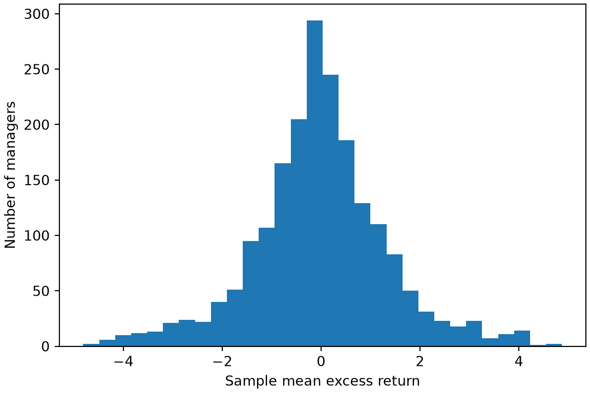
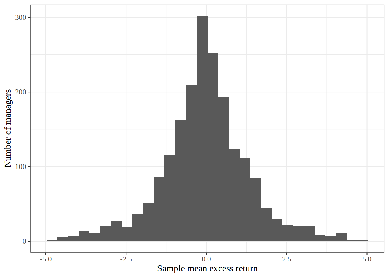
Exercise 2 (Lab: a histogram of the managers’ mean returns) Use the Fund data. Draw a histogram of the sample mean excess return of each of the managers.
import matplotlib.pyplot as pltfund_py_means = fund_py.mean()fig, ax = plt.subplots(figsize=(6, 4), layout="constrained")ax.hist(fund_py_means, bins=30);ax.set_xlabel("Sample mean excess return");ax.set_ylabel("Number of managers");plt.show()
library(ggplot2)# nolint: undesirable_function_linterfund_r_means<-map_dbl(fund_r, mean)fund_r_means_tbl<-tibble(mean =fund_r_means)means_histogram<-fund_r_means_tbl|>ggplot()+aes(mean)+geom_histogram(bins =30)+labs(x ="Sample mean excess return", y ="Number of managers")means_histogram
Figure 1 shows a sharp peak at zero and heavy tails on both sides.
I chose 30 bins, which is 67 managers per bar on average. Far fewer bins would hide the shape inside a few wide bars, and far more would leave most bars with only a few managers, so the outline would look ragged. That is why 30 is a compromise between the two.
Exercise 4 (Lab: test every manager) Use the Fund data. Run the test of Solution 3 for each of the managers, then count the managers whose \(p\)-value is below \(0.05\).
TipHint
The test routine in Python takes a whole table plus an axis, while in R you can apply the test to each column.
The test rejects for 289 of the 2000 managers. If no manager had any skill, each test would reject \(5\%\) of the time, so about 100 managers would be rejected by chance alone. This \(5\%\) figure is why a count of rejected managers at level \(0.05\) cannot by itself identify skilled managers.
The correction rejects 0 of the 2000 managers. It rejects far fewer managers than the uncorrected test did, because it guards against any wrong call across all the tests.
ExrExercise 6 (Lab: the Benjamini–Hochberg procedure)
The method rejects 146 managers, more than the correction of Solution 5 does, because allowing a small share of wrong calls is a weaker aim than allowing none.
G. James, D. Witten, T. Hastie, R. Tibshirani, and J. Taylor, An introduction to statistical learning: With applications in Python. Springer, 2023. doi: 10.1007/978-3-031-38747-0.