Last modified: 2026-11-19
This page holds the code lab for the multiple testing notes.
To work the lab without the solutions, download a stub with only the exercises:
Each solution shows the code in Python and in R.
Section 13.6 of the book [1] is the source of these exercises. The Python code uses pandas, matplotlib, plus SciPy, while the R code uses the tidyverse.
Dataset 1: The fund manager (Fund) data
Monthly excess returns of 2000 fund managers over 50 months make up the Fund data [1, Sec. 13.6]. The data are in data/fund.csv, one column per manager and one row per month, copied from the ISLP Python package. A manager’s excess return is the manager’s return minus a benchmark’s, so a manager with no skill has an excess return of zero on average.
Fund) data
Exercise 1 (Lab: the first manager’s returns)
Exercise 1 (Lab: the first manager’s returns) Use the Fund data. What are the sample mean and sample standard deviation of the excess returns of Manager1?
Hint
Read the file into a table, then apply a summary function to one column.
Solution 1.
Over 50 months, Manager1 has a mean excess return of 3 and a standard deviation of 7.42.
Exercise 2 (Lab: a histogram of the managers’ mean returns)
Exercise 2 (Lab: a histogram of the managers’ mean returns) Use the Fund data. Draw a histogram of the sample mean excess return of each of the managers.
Hint
Summarize each column of the table to get one value per manager, then draw a histogram of those values.
Solution 2. This solution continues Solution 1.
library(ggplot2) # nolint: undesirable_function_linter
fund_r_means <- map_dbl(fund_r, mean)
fund_r_means_tbl <- tibble(mean = fund_r_means)
means_histogram <- fund_r_means_tbl |>
ggplot() +
aes(mean) +
geom_histogram(bins = 30) +
labs(x = "Sample mean excess return", y = "Number of managers")
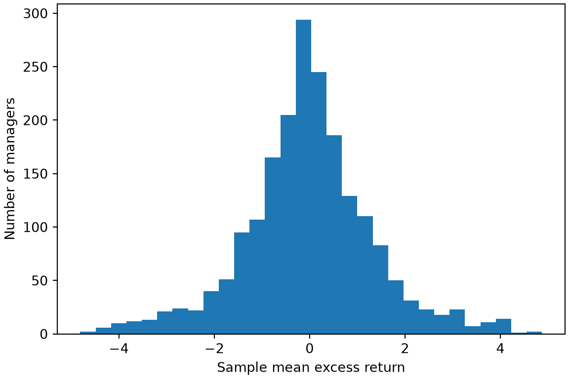
means_histogramFigure 1 shows a sharp peak at zero and heavy tails on both sides.
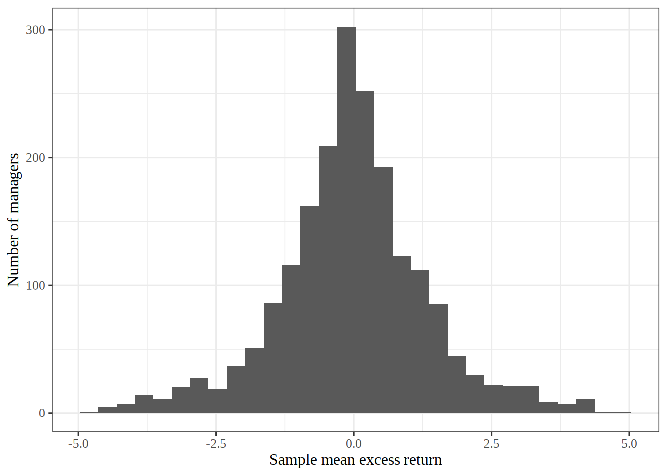
I chose 30 bins, which is 67 managers per bar on average. Far fewer bins would hide the shape inside a few wide bars, and far more would leave most bars with only a few managers, so the outline would look ragged. That is why 30 is a compromise between the two.
Exercise 3 (Lab: test the first manager)
Exercise 3 (Lab: test the first manager) Use the Fund data. Run a one-sample \(t\)-test of the null hypothesis that Manager1 has no skill. What is the \(p\)-value?
Hint
The scipy.stats module has a \(t\)-test in Python, while R has t.test().
Solution 3. This solution continues Solution 2.
The \(p\)-value is 0.0062. At significance level \(0.05\), the test rejects the null hypothesis for this one manager.
Exercise 4 (Lab: test every manager)
Exercise 4 (Lab: test every manager) Use the Fund data. Run the test of Solution 3 for each of the managers, then count the managers whose \(p\)-value is below \(0.05\).
Hint
The test routine in Python takes a whole table plus an axis, while in R you can apply the test to each column.
Solution 4. This solution continues Solution 3.
The test rejects for 289 of the 2000 managers. If no manager had any skill, each test would reject \(5\%\) of the time, so about 100 managers would be rejected by chance alone. This \(5\%\) figure is why a count of rejected managers at level \(0.05\) cannot by itself identify skilled managers.
Exercise 5 (Lab: the Bonferroni correction)
Exercise 5 (Lab: the Bonferroni correction) Use the \(p\)-values of Solution 4. Apply the Bonferroni correction to hold the family-wise error rate at \(0.05\). How many managers does it reject?
Hint
Multiply each \(p\)-value by the count of tests, then compare it with \(0.05\). In R, p.adjust() does the multiplication.
Solution 5. This solution continues Solution 4.
The correction rejects 0 of the 2000 managers. It rejects far fewer managers than the uncorrected test did, because it guards against any wrong call across all the tests.
Exercise 6 (Lab: the Benjamini–Hochberg procedure)
Exercise 6 (Lab: the Benjamini–Hochberg procedure) Use the \(p\)-values of Solution 4. Apply the Benjamini–Hochberg procedure to hold the false discovery rate at \(0.1\). How many managers does it reject?
Hint
The scipy.stats module adjusts \(p\)-values in Python, while R’s p.adjust() takes the method "BH".
Solution 6. This solution continues Solution 5.
The method rejects 146 managers, more than the correction of Solution 5 does, because allowing a small share of wrong calls is a weaker aim than allowing none.