Last modified: 2026-11-19
Source
This material was a section of the logistic regression page. It carries the same sources: Brian Hutchinson’s Fall 2025 lecture notes, Kameron Decker Harris’ 2022 weekly notes and Logan Sizemore’s Spring 2025 lectures, as described there.
A fitted coefficient is an estimate: another sample from the same population would give a different value, and its sampling distribution describes how much it varies. The matrix \(\qform{W}{\design}\) that Newton’s method uses to compute its step also gives the size of that variation. Where the log-likelihood curves sharply at \(\hvcoef\), \(\qform{W}{\design}\) is large and the standard errors are small; where it is nearly flat, the standard errors are large.
Remark 1 (Inference for logistic regression)
Remark 1 (Inference for logistic regression). The statistics notes’ page Inference for Logistic Regression covers the deviance, the null deviance, the likelihood ratio test of the slopes, and the Wald interval for a fitted logistic coefficient. It shows that the drop from the null deviance to the deviance is the likelihood ratio statistic. It also shows that, for a large sample, the fitted coefficients \(\hvcoef\) are approximately Gaussian with mean \(\vcoef\) and covariance \(\inv{\tp{\design} W \design}\) (its approximate distribution theorem), where \(W\) is the weight matrix in the logistic Hessian theorem. In that result the weights \(\prob_i \paren{1 - \prob_i}\) are computed from the true probabilities; the standard errors, like the Newton step, use the weights computed from the fitted probabilities instead.
Statistical software fits logistic regression by the Newton iteration of part 2 of the Newton and IRLS exercise. This section uses it on stock market data, to predict whether the market rises on a given day.
Dataset 1: The stock market (Smarket) data
Daily percentage returns of the S&P 500 stock index on 1250 trading days from 2001 to 2005 make up the Smarket data [1, Sec. 4.7]. The data are in data/smarket.csv, one row per trading day, copied from the ISLP Python package. The columns this course uses are:
Direction: the outcome, whether the index rose (Up) or fell (Down) that day.Lag1 to Lag5: the percentage returns on each of the five previous trading days.Volume: the number of shares traded on the previous day, in billions.Year: the year of the trading day.The Today column, the day’s own return, is not a predictor, because Direction is Down exactly when Today is negative.
The Date column, the calendar date of each trading day, is not used by the exercises; it names the day that a row describes, from 2001-01-10 to 2005-12-30. The ISLP copy has no dates. The dates were recovered by matching Today against the S&P 500 daily returns in the sp500ret data of the rugarch package [2], after converting those log returns to percentage returns. The script tools/add_smarket_dates.R does the match. It stops unless exactly one run of trading days agrees with all 1250 values of Today, to within 0.0005 percentage points, the rounding of Today.
Smarket) data
[1] 1250 10
Variable type: character
| skim_variable | n_missing | complete_rate | min | max | empty | n_unique | whitespace |
|---|---|---|---|---|---|---|---|
| Direction | 0 | 1 | 2 | 4 | 0 | 2 | 0 |
Variable type: Date
| skim_variable | n_missing | complete_rate | min | max | median | n_unique |
|---|---|---|---|---|---|---|
| Date | 0 | 1 | 2001-01-10 | 2005-12-30 | 2003-07-10 | 1250 |
Variable type: numeric
| skim_variable | n_missing | complete_rate | mean | sd | p0 | p25 | p50 | p75 | p100 |
|---|---|---|---|---|---|---|---|---|---|
| Year | 0 | 1 | 2003.02 | 1.41 | 2001.00 | 2002.00 | 2003.00 | 2004.00 | 2005.00 |
| Lag1 | 0 | 1 | 0.00 | 1.14 | -4.92 | -0.64 | 0.04 | 0.60 | 5.73 |
| Lag2 | 0 | 1 | 0.00 | 1.14 | -4.92 | -0.64 | 0.04 | 0.60 | 5.73 |
| Lag3 | 0 | 1 | 0.00 | 1.14 | -4.92 | -0.64 | 0.04 | 0.60 | 5.73 |
| Lag4 | 0 | 1 | 0.00 | 1.14 | -4.92 | -0.64 | 0.04 | 0.60 | 5.73 |
| Lag5 | 0 | 1 | 0.01 | 1.15 | -4.92 | -0.64 | 0.04 | 0.60 | 5.73 |
| Volume | 0 | 1 | 1.48 | 0.36 | 0.36 | 1.26 | 1.42 | 1.64 | 3.15 |
| Today | 0 | 1 | 0.00 | 1.14 | -4.92 | -0.64 | 0.04 | 0.60 | 5.73 |
Year Lag1 Lag2 Lag3 Lag4 Lag5 Volume Today Direction Date
0 2001 0.381 -0.192 -2.624 -1.055 5.010 1.19130 0.959 Up 2001-01-10
1 2001 0.959 0.381 -0.192 -2.624 -1.055 1.29650 1.032 Up 2001-01-11
2 2001 1.032 0.959 0.381 -0.192 -2.624 1.41120 -0.623 Down 2001-01-12
3 2001 -0.623 1.032 0.959 0.381 -0.192 1.27600 0.614 Up 2001-01-16
4 2001 0.614 -0.623 1.032 0.959 0.381 1.20570 0.213 Up 2001-01-17
... ... ... ... ... ... ... ... ... ... ...
1245 2005 0.422 0.252 -0.024 -0.584 -0.285 1.88850 0.043 Up 2005-12-23
1246 2005 0.043 0.422 0.252 -0.024 -0.584 1.28581 -0.955 Down 2005-12-27
1247 2005 -0.955 0.043 0.422 0.252 -0.024 1.54047 0.130 Up 2005-12-28
1248 2005 0.130 -0.955 0.043 0.422 0.252 1.42236 -0.298 Down 2005-12-29
1249 2005 -0.298 0.130 -0.955 0.043 0.422 1.38254 -0.489 Down 2005-12-30
[1250 rows x 10 columns]
<class 'pandas.DataFrame'>
RangeIndex: 1250 entries, 0 to 1249
Data columns (total 10 columns):
# Column Non-Null Count Dtype
--- ------ -------------- -----
0 Year 1250 non-null int64
1 Lag1 1250 non-null float64
2 Lag2 1250 non-null float64
3 Lag3 1250 non-null float64
4 Lag4 1250 non-null float64
5 Lag5 1250 non-null float64
6 Volume 1250 non-null float64
7 Today 1250 non-null float64
8 Direction 1250 non-null str
9 Date 1250 non-null str
dtypes: float64(7), int64(1), str(2)
memory usage: 97.8 KB
Year Lag1 Lag2 Lag3 Lag4 Lag5 Volume Today
count 1250.000000 1250.000000 1250.000000 1250.000000 1250.000000 1250.00000 1250.000000 1250.000000
mean 2003.016000 0.003834 0.003919 0.001716 0.001636 0.00561 1.478305 0.003138
std 1.409018 1.136299 1.136280 1.138703 1.138774 1.14755 0.360357 1.136334
min 2001.000000 -4.922000 -4.922000 -4.922000 -4.922000 -4.92200 0.356070 -4.922000
25% 2002.000000 -0.639500 -0.639500 -0.640000 -0.640000 -0.64000 1.257400 -0.639500
50% 2003.000000 0.039000 0.039000 0.038500 0.038500 0.03850 1.422950 0.038500
75% 2004.000000 0.596750 0.596750 0.596750 0.596750 0.59700 1.641675 0.596750
max 2005.000000 5.733000 5.733000 5.733000 5.733000 5.73300 3.152470 5.733000
Year 0
Lag1 0
Lag2 0
Lag3 0
Lag4 0
Lag5 0
Volume 0
Today 0
Direction 0
Date 0
dtype: int64
Exercise 1 (Predicting the direction of the stock market)
Exercise 1 (Predicting the direction of the stock market) Use the Smarket data. Fit a logistic regression for the probability that Direction is Up, with the five lagged returns and Volume as predictors, on the days before 2005 only.
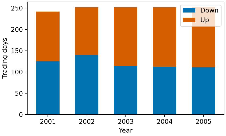
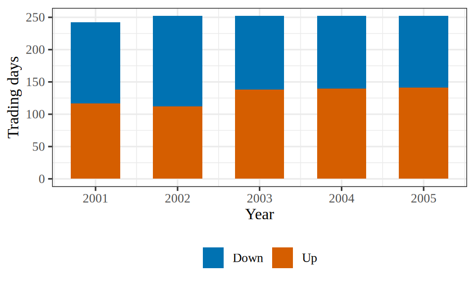
Figure 1 plots the number of trading days in each year by Direction, including the days of 2005 that the fit leaves out.
sf_data <- readr::read_csv("data/smarket.csv", show_col_types = FALSE)
sf_fills <- c(Down = "#0072B2", Up = "#D55E00")
sf_data |>
ggplot2::ggplot(ggplot2::aes(Year, fill = Direction)) +
ggplot2::geom_bar(width = 0.6) +
ggplot2::scale_fill_manual(values = sf_fills) +
ggplot2::labs(x = "Year", y = "Trading days", fill = NULL)import matplotlib.pyplot as plt
import pandas as pd
smarket_sf = pd.read_csv("data/smarket.csv")
counts_sf = smarket_sf.groupby(["Year", "Direction"]).size().unstack()
fig, ax = plt.subplots(figsize=(5, 3), layout="constrained")
ax.bar(counts_sf.index, counts_sf["Down"], color="#0072B2", width=0.6,
label="Down");
ax.bar(counts_sf.index, counts_sf["Up"], bottom=counts_sf["Down"],
color="#D55E00", width=0.6, label="Up");
ax.set_xlabel("Year");
ax.set_ylabel("Trading days");
ax.legend();
plt.show()Solution 1.
'data.frame': 1250 obs. of 10 variables:
$ Year : int 2001 2001 2001 2001 2001 2001 2001 2001 2001 2001 ...
$ Lag1 : num 0.381 0.959 1.032 -0.623 0.614 ...
$ Lag2 : num -0.192 0.381 0.959 1.032 -0.623 ...
$ Lag3 : num -2.624 -0.192 0.381 0.959 1.032 ...
$ Lag4 : num -1.055 -2.624 -0.192 0.381 0.959 ...
$ Lag5 : num 5.01 -1.055 -2.624 -0.192 0.381 ...
$ Volume : num 1.19 1.3 1.41 1.28 1.21 ...
$ Today : num 0.959 1.032 -0.623 0.614 0.213 ...
$ Direction: chr "Up" "Up" "Down" "Up" ...
$ Date : chr "2001-01-10" "2001-01-11" "2001-01-12" "2001-01-16" ...
(Intercept) Lag1 Lag2 Lag3 Lag4 Lag5
0.191212621 -0.054178292 -0.045805334 0.007200118 0.006440875 -0.004222672
Volume
-0.116256960
Year Lag1 Lag2 Lag3 Lag4 Lag5 Volume Today Direction Date
0 2001 0.381 -0.192 -2.624 -1.055 5.010 1.1913 0.959 Up 2001-01-10
1 2001 0.959 0.381 -0.192 -2.624 -1.055 1.2965 1.032 Up 2001-01-11
2 2001 1.032 0.959 0.381 -0.192 -2.624 1.4112 -0.623 Down 2001-01-12
Intercept 0.191
Lag1 -0.054
Lag2 -0.046
Lag3 0.007
Lag4 0.006
Lag5 -0.004
Volume -0.116
dtype: float64
Exercise 2 (Predicting the direction of the stock market (part 1b))
Exercise 2 (Predicting the direction of the stock market (part 1b)) Use the setup of Exercise 1.
Predict Direction for each day in 2005 from the fit of Exercise 1, predicting Up when the predicted probability is above \(0.5\).
Solution 2. This continues Solution 1.
Exercise 3 (Predicting the direction of the stock market (part 1c))
Exercise 3 (Predicting the direction of the stock market (part 1c)) Use the setup of Exercise 1.
On what proportion of the 2005 days is the prediction of Exercise 2 correct?
Solution 3. This continues Solution 1 and Solution 2.
[1] 0.4801587
# A 95% interval for an accuracy: the proportion plus or minus
# 1.96 standard errors, which is accurate when the number of test days
# is in the hundreds.
n_test <- length(actual)
bounds <- c(lower = -1, upper = 1)
z_crit <- qnorm(0.975)
se_accuracy <- sqrt(accuracy * (1 - accuracy) / n_test)
ci_accuracy <- accuracy + bounds * z_crit * se_accuracyaccuracy: 0.48
(0.418, 0.542)
The fitted logistic regression predicts the correct label on 48% of the 252 days in 2005 (95% interval [41.8, 54.2]%).
Exercise 4 (Predicting the direction of the stock market (part 2))
Exercise 4 (Predicting the direction of the stock market (part 2)) Use the setup of Exercise 1.
Compare the proportion correct of Exercise 3 with that of the rule that predicts Up on every day.
Solution 4.
always_up <- mean(actual == "Up")
se_always_up <- sqrt(always_up * (1 - always_up) / n_test)
ci_always_up <- always_up + bounds * z_crit * se_always_up
# Both rules are scored on the same days, so the paired difference in
# correctness, day by day, has a t interval for its mean.
hit_model <- as.integer(pred == actual)
hit_up <- as.integer(actual == "Up")
diff_hit <- hit_model - hit_up
t_crit <- qt(0.975, n_test - 1)
se_diff <- sd(diff_hit) / sqrt(n_test)
ci_vs_up <- mean(diff_hit) + bounds * t_crit * se_diffPredicting Up on every day is right on 56% of the 2005 days (95% interval [49.8, 62.1]%). Each interval is the proportion plus or minus 1.96 standard errors, \(\sqrt{\eprob (1 - \eprob) / n}\). The two rules are scored on the same days, so their difference is taken day by day: the accuracy of the logistic regression minus that of the constant rule is -7.9 percentage points (95% interval [-18.2, 2.3]). The intervals describe sampling variation across the test days in 2005, not across training sets.
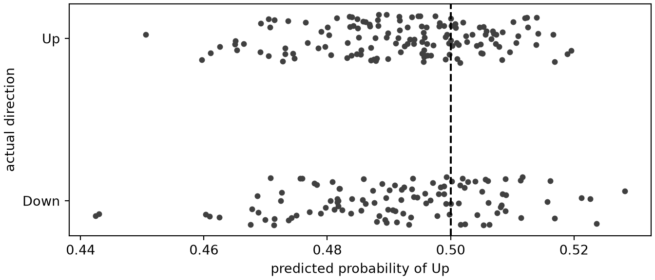
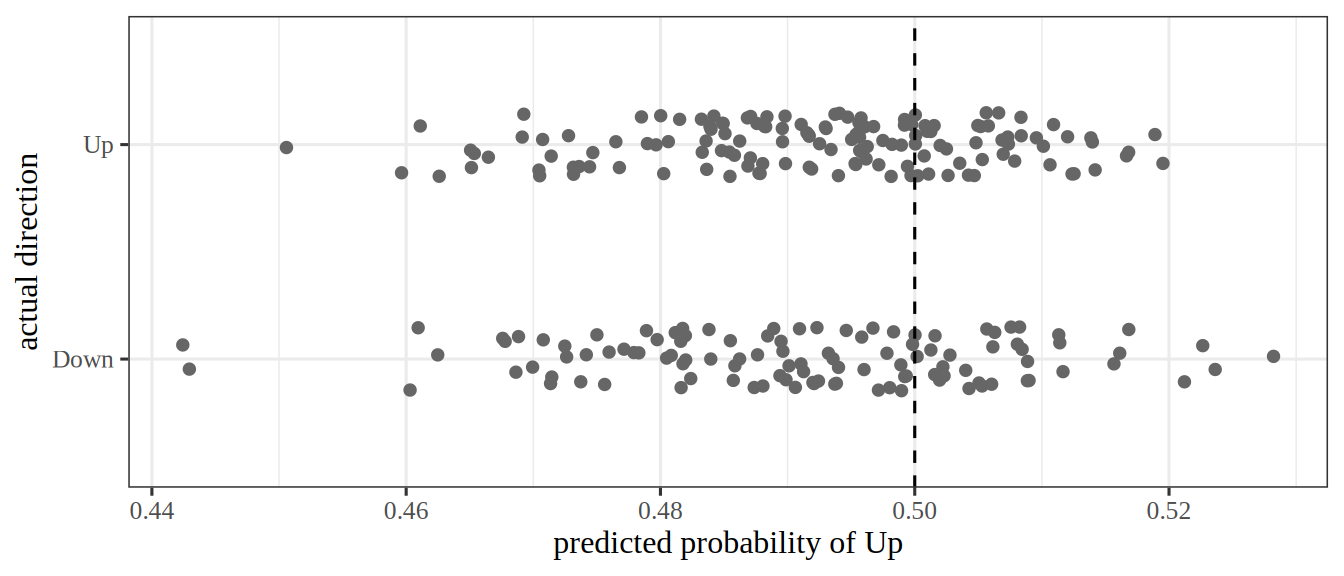
The fitted model is right less often than the rule that ignores every predictor, but the interval for the difference includes 0, so these 252 days do not show that the fitted model is worse. Its predicted probabilities are all between 0.44 and 0.53: no day in 2005 gets a probability of Up far from \(0.5\). Figure 2 shows that the days that went up and the days that went down get nearly the same predicted probabilities.
import matplotlib.pyplot as plt
rng_strip = np.random.default_rng(571)
row = np.where(actual_py == "Up", 1, 0) + rng_strip.uniform(-0.15, 0.15, len(actual_py))
fig, ax = plt.subplots(figsize=(7, 3), layout="constrained")
ax.scatter(p_py, row, color="0.25", s=12);
ax.axvline(0.5, color="black", linestyle="--");
ax.set_yticks([0, 1], ["Down", "Up"]);
ax.set_xlabel("predicted probability of Up");
ax.set_ylabel("actual direction");
plt.show()Exercise 5 (Fitting the stock market model by gradient descent)
Exercise 5 (Fitting the stock market model by gradient descent) Exercise 1 fitted the 2001 to 2004 Smarket days with R’s glm() and statsmodels’ GLM. Fit the same logistic regression with the gradient descent of the exercise on fitting by gradient descent, standardizing the six predictors with the training days’ means and standard deviations, starting from \(\vcoef = \vzero\), with step size \(\learnrate = 0.5\) for \(2{,}000\) steps.
Solution 5.
cols <- c("Lag1", "Lag2", "Lag3", "Lag4", "Lag5", "Volume")
smarket_train <- smarket |>
dplyr::filter(train) |>
dplyr::select(dplyr::all_of(cols))
smarket_test <- smarket |>
dplyr::filter(!train) |>
dplyr::select(dplyr::all_of(cols))
mu <- colMeans(smarket_train)
sdev <- apply(smarket_train, 2, sd)
# nolint start: object_name_linter.
Xs <- cbind(1, scale(smarket_train, mu, sdev))
Xte <- cbind(1, scale(smarket_test, mu, sdev))
# nolint end
y_tr <- smarket$up[train]
sig <- function(z) 0.5 * (1 + tanh(0.5 * z))
b <- rep(0, ncol(Xs))
for (i in 1:2000) {
b <- b - 0.5 * drop(t(Xs) %*% (sig(drop(Xs %*% b)) - y_tr)) / length(y_tr)
}
b Lag1 Lag2 Lag3 Lag4 Lag5
0.032104744 -0.066621178 -0.056325934 0.008874033 0.007939830 -0.005248037
Volume
-0.031112330
cols = ["Lag1", "Lag2", "Lag3", "Lag4", "Lag5", "Volume"]
tr = smarket_py[train_py]
mu, sd = tr[cols].mean(), tr[cols].std()
Xs_py = np.column_stack([np.ones(len(tr)), ((tr[cols] - mu) / sd).to_numpy()])
Xte_py = np.column_stack(
[np.ones((~train_py).sum()), ((smarket_py.loc[~train_py, cols] - mu) / sd).to_numpy()]
)
y_tr_py = tr["up"].to_numpy()
sig = lambda z: 0.5 * (1 + np.tanh(0.5 * z))
b_py = np.zeros(Xs_py.shape[1])
for _ in range(2000):
b_py = b_py - 0.5 * Xs_py.T @ (sig(Xs_py @ b_py) - y_tr_py) / len(y_tr_py)
print("standardized:", np.round(b_py, 3))standardized: [ 0.032 -0.067 -0.056 0.009 0.008 -0.005 -0.031]
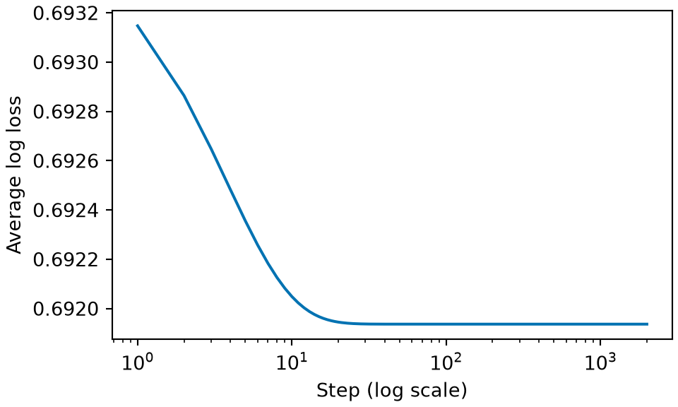
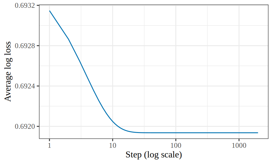
Figure 3 plots the average log loss at each step of the loop above.
gdl_steps <- 2000
gdl_loss <- numeric(gdl_steps)
gdl_ncol <- ncol(Xs)
gdl_b <- rep(0, gdl_ncol)
for (i in seq_len(gdl_steps)) {
gdl_z <- drop(Xs %*% gdl_b)
gdl_p <- sig(gdl_z)
gdl_pt <- ifelse(y_tr == 1, gdl_p, 1 - gdl_p)
gdl_loss[i] <- mean(-log(gdl_pt))
gdl_grad <- drop(t(Xs) %*% (gdl_p - y_tr)) / length(y_tr)
gdl_b <- gdl_b - 0.5 * gdl_grad
}
gdl_seq <- seq_len(gdl_steps)
gdl_path <- tibble::tibble(step = gdl_seq, loss = gdl_loss)
gdl_path |>
ggplot2::ggplot(ggplot2::aes(step, loss)) +
ggplot2::geom_line(colour = "#0072B2") +
ggplot2::scale_x_log10() +
ggplot2::labs(x = "Step (log scale)", y = "Average log loss")import matplotlib.pyplot as plt
import numpy as np
b_gdl = np.zeros(Xs_py.shape[1])
loss_gdl = []
for _ in range(2000):
p_gdl = sig(Xs_py @ b_gdl)
p_true = np.where(y_tr_py == 1, p_gdl, 1 - p_gdl)
loss_gdl.append(np.mean(-np.log(p_true)))
grad_gdl = Xs_py.T @ (p_gdl - y_tr_py) / len(y_tr_py)
b_gdl = b_gdl - 0.5 * grad_gdl
fig, ax = plt.subplots(figsize=(5, 3), layout="constrained")
ax.plot(np.arange(1, 2001), loss_gdl, color="#0072B2");
ax.set_xscale("log");
ax.set_xlabel("Step (log scale)");
ax.set_ylabel("Average log loss");
plt.show()Exercise 6 (Fitting the stock market model by gradient descent (part 1b))
Exercise 6 (Fitting the stock market model by gradient descent (part 1b)) Use the setup of Exercise 5.
Convert the coefficients of the fit of Exercise 5 back to the original units of the predictors.
Solution 6. This continues Solution 5.
Lag1 Lag2 Lag3 Lag4
gradient_descent 0.1912126 -0.05417829 -0.04580533 0.007200118 0.006440875
library_fit 0.1912126 -0.05417829 -0.04580533 0.007200118 0.006440875
Lag5 Volume
gradient_descent -0.004222672 -0.116257
library_fit -0.004222672 -0.116257
[1] 1
gradient descent: [ 0.191 -0.054 -0.046 0.007 0.006 -0.004 -0.116]
library fit: [ 0.191 -0.054 -0.046 0.007 0.006 -0.004 -0.116]
same predictions: 1.0
Exercise 7 (Fitting the stock market model by gradient descent: how close?)
Exercise 7 (Fitting the stock market model by gradient descent: how close?) Use the setup of Exercise 5.
What is the largest absolute difference between the gradient descent coefficients and those of Exercise 1?
Solution 7. The largest absolute difference between the two sets of coefficients is 4.3e-10.
Exercise 8 (Fitting the stock market model by gradient descent (part 2))
Exercise 8 (Fitting the stock market model by gradient descent (part 2)) Use the setup of Exercise 5.
On what proportion of the 2005 days do the two fits make the same prediction?
Solution 8. The two fits make the same prediction on 100% of the 2005 days. Gradient descent ends near the glm() fit for three reasons.
L step_bound
0.2823152 7.0842810
glm() converged, with every fitted probability between 0.4 and 0.6.Standardizing the predictors puts the coefficients on similar scales, so one step size suits all of them.
Watch
Hastie and Tibshirani fit logistic regression in code in their Python lab [3].
Read
The Chapter 4 lab of James et al. [1], Ch04-classification-lab.ipynb in ISLP_labs, fits the same logistic regression to the Smarket data, and then compares it with four other classifiers on the same data [1, Sec. 4.7]. The discriminant analysis chapter names three of them. The classification lab works the logistic regression part.
The fits so far assumed that the likelihood has a finite maximizer. When a hyperplane puts every observation of one class on one side and every observation of the other class on the other side, the likelihood has no finite maximizer [4]. Any \(\ninputvars + 1\) points in general position in \(\reals^{\ninputvars}\) can be split this way, whatever their classes, so such a split is common when the sample is small relative to the number of predictors. Fitting software still stops and reports finite coefficients, and the Wald test and the likelihood ratio test reach opposite conclusions.
Exercise 9 (When the data separate perfectly)
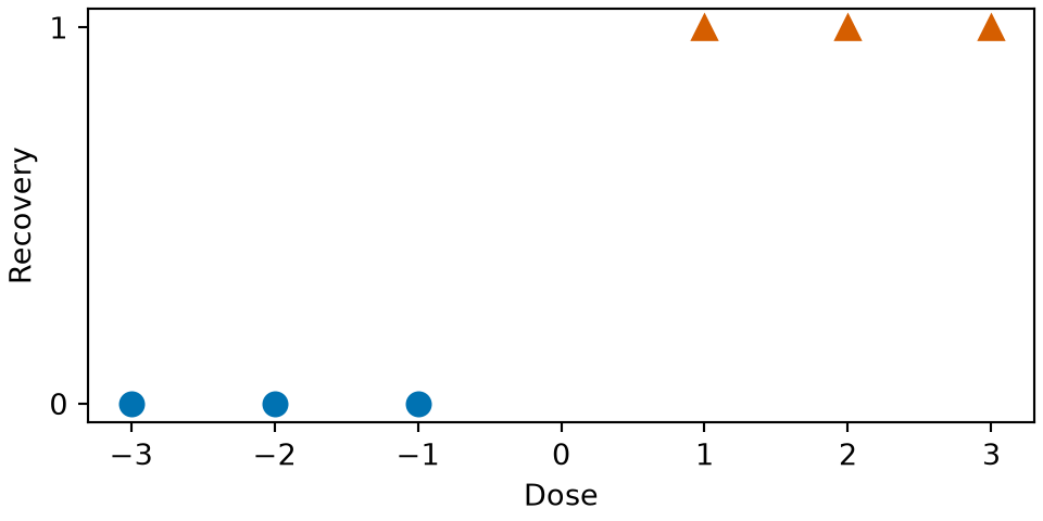
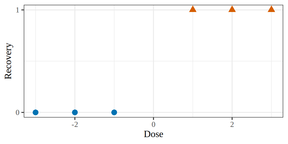
Exercise 9 (When the data separate perfectly) A second trial, of six patients, records a dose \(\predvar\) and recovery \(y\):
| \(\predvar\) | \(-3\) | \(-2\) | \(-1\) | \(+1\) | \(+2\) | \(+3\) |
|---|---|---|---|---|---|---|
| \(y\) | \(0\) | \(0\) | \(0\) | \(1\) | \(1\) | \(1\) |
Every patient with a negative dose failed to recover, and every patient with a positive dose recovered.
Show, as in part 3 of the worked fit exercise, that the score for \(\coef{0}\) is \(0\) at \(\coef{0} = 0\) for every \(\coef{1}\).
Figure 4 plots the six patients.
sep_dose <- c(-3, -2, -1, 1, 2, 3)
sep_y <- c(0, 0, 0, 1, 1, 1)
sep_recovery <- factor(sep_y)
sep_fig <- tibble::tibble(dose = sep_dose, y = sep_y, recovery = sep_recovery)
sep_colours <- c("0" = "#0072B2", "1" = "#D55E00")
sep_shapes <- c("0" = 16, "1" = 17)
sep_breaks <- c(0, 1)
sep_fig |>
ggplot2::ggplot(ggplot2::aes(dose, y, colour = recovery, shape = recovery)) +
ggplot2::geom_point(size = 3) +
ggplot2::scale_colour_manual(values = sep_colours, guide = "none") +
ggplot2::scale_shape_manual(values = sep_shapes, guide = "none") +
ggplot2::scale_y_continuous(breaks = sep_breaks) +
ggplot2::labs(x = "Dose", y = "Recovery")import matplotlib.pyplot as plt
fig, ax = plt.subplots(figsize=(5, 2.5), layout="constrained")
dose_sep = [-3, -2, -1]
ax.plot(dose_sep, [0, 0, 0], "o", color="#0072B2", markersize=8);
ax.plot([1, 2, 3], [1, 1, 1], "^", color="#D55E00", markersize=8);
ax.set_yticks([0, 1]);
ax.set_xlabel("Dose");
ax.set_ylabel("Recovery");
plt.show()Solution 9. In Exercise 9, the doses of the three patients with \(\outvar = 0\) are the negatives of the doses of the three with \(\outvar = 1\). At \(\coef{0} = 0\), \(\prob_i = \sigmoidf{\coef{1} \predvar_i}\), and \(\sigmoidf{-z} + \sigmoidf{z} = 1\) (part 2 of the sigmoid properties exercise), so
\[ \begin{aligned} \sumin \prob_i &= \sum_{k=1}^{3} \sb{\sigmoidf{-k\coef{1}} + \sigmoidf{k\coef{1}}} && \text{(pair dose } -k \text{ with dose } k \text{)} \\ &= 3 && \text{(each pair sums to } 1 \text{)} \\ &= \sumin \outvar_i. \end{aligned} \]
So the score for \(\coef{0}\), \(\sumin \paren{\outvar_i - \prob_i}\), is \(0\) for every \(\coef{1}\).
Exercise 10 (When the data separate perfectly: the log-likelihood)
Exercise 10 (When the data separate perfectly: the log-likelihood) Use the setup of Exercise 9.
Show that with \(\coef{0} = 0\) the log-likelihood is
\[ \llik(\coef{1}) = 2\log\sigmoidf{\coef{1}} + 2\log\sigmoidf{2\coef{1}} + 2\log\sigmoidf{3\coef{1}}. \]
Solution 10. With \(\coef{0} = 0\), a patient with \(\outvar_i = 1\) and dose \(k\) contributes \(\log\sigmoidf{k\coef{1}}\). A patient with \(\outvar_i = 0\) and dose \(-k\) contributes
\[ \begin{aligned} \log\sb{1 - \sigmoidf{-k\coef{1}}} &= \log\sigmoidf{k\coef{1}}. && \text{(} 1 - \sigmoidf{-z} = \sigmoidf{z} \text{)} \end{aligned} \]
Each \(k \in \set{1, 2, 3}\) occurs once in each group, so each \(\log\sigmoidf{k\coef{1}}\) appears twice, which gives the stated \(\llik\).
Exercise 11 (When the data separate perfectly: an increasing log-likelihood)
Exercise 11 (When the data separate perfectly: an increasing log-likelihood) Use the setup of Exercise 10.
Show that \(\llik(\coef{1})\) is strictly increasing.
Solution 11. For each \(k\), the derivative of \(\log\sigmoidf{kz}\) with respect to \(z\) is \(k\sb{1 - \sigmoidf{kz}}\), so
\[ \begin{aligned} \score(\coef{1}) &= 2\sb{1 - \sigmoidf{\coef{1}}} + 4\sb{1 - \sigmoidf{2\coef{1}}} + 6\sb{1 - \sigmoidf{3\coef{1}}} && \text{(differentiate each term)} \\ &= 2\sigmoidf{-\coef{1}} + 4\sigmoidf{-2\coef{1}} + 6\sigmoidf{-3\coef{1}} && \text{(} 1 - \sigmoidf{z} = \sigmoidf{-z} \text{)} \\ &> 0 && \text{(} \sigmoid > 0 \text{)} \end{aligned} \]
for every \(\coef{1}\), so \(\llik\) is strictly increasing.
Exercise 12 (When the data separate perfectly: the supremum)
Exercise 12 (When the data separate perfectly: the supremum) Use the setup of Exercise 11.
Find \(\sup_{\coef{1}} \llik(\coef{1})\).
Solution 12. As \(\coef{1} \to \infty\), each \(\sigmoidf{k\coef{1}} \to 1\), so each \(\log\sigmoidf{k\coef{1}} \to 0\). So \(\sup_{\coef{1}} \llik(\coef{1}) = 0\), and the supremum of the likelihood is \(1\).
Exercise 13 (When the data separate perfectly: is the supremum attained?)
Exercise 13 (When the data separate perfectly: is the supremum attained?) Use the setup of Exercise 11.
Is the supremum of the log-likelihood attained at any \((\coef{0}, \coef{1})\)?
Solution 13. No. At any finite \((\coef{0}, \coef{1})\), every fitted probability is strictly between \(0\) and \(1\), so each of the six terms of the log-likelihood is negative, and \(\llik(\coef{0}, \coef{1}) < 0\). So no \((\coef{0}, \coef{1})\) maximizes the likelihood, and the maximum likelihood estimate does not exist.
Definition 1 (Separated data (completely separated data))
Definition 1 (Separated data (completely separated data)) A dataset \((\vx_1, \outvar_1), \ldots, (\vx_\nobs, \outvar_\nobs)\) with \(\outvar_i \in \set{0, 1}\), where each \(\vx_i\) includes the leading \(1\) for the intercept, is separated, also called completely separated [4], when some \(\vcoef\) has \(\dprod{\vcoef}{\vx_i} > 0\) for every \(i\) with \(\outvar_i = 1\) and \(\dprod{\vcoef}{\vx_i} < 0\) for every \(i\) with \(\outvar_i = 0\). Such a \(\vcoef\) is said to separate the data.
Example 1 (A separated dataset and one that is not)
Example 1 (A separated dataset and one that is not) The six patients of Exercise 9 are separated: \(\vcoef = \tp{(0, 1)}\) gives \(\dprod{\vcoef}{\vx_i} = \predvar_i\), which is \(1\), \(2\) or \(3\) for the patients who recovered and \(-1\), \(-2\) or \(-3\) for those who did not.
The six patients of the worked fit exercise are not separated. Each group contains a patient who recovered and a patient who did not, and those two patients have the same \(\vx_i = \tp{(1, \predvar_i)}\), so \(\dprod{\vcoef}{\vx_i}\) cannot be positive for one and negative for the other.
Definition 2 (Quasi-completely separated data)
Definition 2 (Quasi-completely separated data) A dataset with \(\outvar_i \in \set{0, 1}\) is quasi-completely separated [4] when it is not separated, but some \(\vcoef \ne \vzero\) has \(\dprod{\vcoef}{\vx_i} \ge 0\) for every \(i\) with \(\outvar_i = 1\) and \(\dprod{\vcoef}{\vx_i} \le 0\) for every \(i\) with \(\outvar_i = 0\).
Example 2 (Four patients, quasi-completely separated)
Example 2 (Four patients, quasi-completely separated) Take four patients with doses \(\predvar = -1, 0, 0, 1\) and recoveries \(\outvar = 0, 0, 1, 1\). They are not separated: the two patients with dose \(0\) have the same \(\vx_i\) and different outcomes. The vector \(\vcoef = \tp{(0, 1)}\) gives \(\dprod{\vcoef}{\vx_i} = -1, 0, 0, 1\), which is \(\ge 0\) for both patients who recovered and \(\le 0\) for both who did not, so the data are quasi-completely separated.
Estimate Std. Error z value Pr(>|z|)
(Intercept) 8.146903e-18 1.414214 5.760730e-18 1.000000
x 1.956607e+01 7604.235498 2.573049e-03 0.997947
glm() reports a slope of 19.6, with a standard error of 7604: the same symptoms as for the separated trial of Exercise 9. For quasi-completely separated data, too, the maximum likelihood estimate does not exist [4].
Exercise 14 (When the data separate perfectly (part 2))
Exercise 14 (When the data separate perfectly (part 2)) Use the setup of Exercise 9.
Now take any separated dataset, and suppose \(\vcoef\) separates it. Show that replacing \(\vcoef\) by \(c\vcoef\), for any \(c > 1\), strictly increases the likelihood.
Solution 14. By the margin form theorem, each observation’s contribution to the log-likelihood is \(-\log\paren{1 + \e{-m_i}}\), with the margin \(m_i = \signoutvar_i \dprod{\vcoef}{\vx_i}\) and \(\signoutvar_i = 2\outvar_i - 1 \in \set{-1, +1}\), so
\[ \llik(\vcoef) = -\sumin \log\paren{1 + \e{-m_i}}. \]
This margin of an observation is not the margin of a separating hyperplane, which does not change when \(\vcoef\) is scaled.
Separation says that every margin is positive: \(m_i > 0\) for all \(i\). Scaling \(\vcoef\) to \(c\vcoef\) multiplies every \(m_i\) by \(c\), so for \(c > 1\) every \(m_i\) increases. Each term \(-\log\paren{1 + \e{-m}}\) is strictly increasing in \(m\), so every term increases. Hence \(\llik(c\vcoef) > \llik(\vcoef)\).
Exercise 15 (When the data separate perfectly: the supremum in general)
Exercise 15 (When the data separate perfectly: the supremum in general) Use the setup of Exercise 14.
Find the supremum of the log-likelihood.
Solution 15. Every term \(-\log\paren{1 + \e{-m_i}}\) of Solution 14 is negative, so \(\llik < 0\) at every finite parameter vector. Along the ray \(c\vcoef\), each term tends to \(0\) as \(c \to \infty\), because \(c m_i \to \infty\). So the supremum of the log-likelihood is \(0\), and the supremum of the likelihood is \(1\).
Exercise 16 (When the data separate perfectly: no maximizer in general)
Exercise 16 (When the data separate perfectly: no maximizer in general) Use the setup of Exercise 15.
Show that no finite parameter vector attains that supremum.
Solution 16. In Solution 15, every term of \(\llik\) is negative, so \(\llik < 0\) at every finite parameter vector, while the supremum is \(0\). So no finite parameter vector attains the supremum of the log-likelihood, or that of the likelihood. Solution 12 and Solution 13 were this argument for one six-patient dataset.
Exercise 17 (When the data separate perfectly (part 3))
Exercise 17 (When the data separate perfectly (part 3)) Use the setup of Exercise 9.
At \(\coef{0} = 0\), the observed information \(\tp{\design} W \design\) is diagonal, and its entry for \(\coef{1}\) is
\[ \oinff{\coef{1}} = \sumin \predvar_i^2\,\prob_i(1 - \prob_i). \]
Evaluate \(\oinff{\coef{1}}\) at \(\coef{1} = 1, 2, 5, 10, 20\), and the standard error \(1/\sqrt{\oinff{\coef{1}}}\) that a fitting routine would report there.
Solution 17. In Exercise 17, the off-diagonal entry of \(\tp{\design} W \design\) is \(\sumin \predvar_i \prob_i (1 - \prob_i)\), which is \(0\) at \(\coef{0} = 0\) because the doses \(k\) and \(-k\) have the same weight \(\sigmoidf{k\coef{1}}\sigmoidf{-k\coef{1}}\). So the standard error of \(\coef{1}\), the square root of the corresponding diagonal entry of \(\inv{\tp{\design} W \design}\), is \(1/\sqrt{\oinff{\coef{1}}}\). At the five values:
sep <- tibble::tibble(x = c(-3, -2, -1, 1, 2, 3), y = c(0, 0, 0, 1, 1, 1))
sep_info <- function(b1) {
p <- plogis(b1 * sep$x)
sum(sep$x^2 * p * (1 - p))
}
sep_b1 <- c(1, 2, 5, 10, 20)
sep_i <- vapply(sep_b1, sep_info, numeric(1))
sep_se <- 1 / sqrt(sep_i)
# Typeset a number for the page: plain if it is not tiny,
# and as $m \times 10^{e}$ when its exponent is -4 or lower.
sep_num <- function(v, digits = 3) {
v <- signif(v, digits)
e <- floor(log10(abs(v)))
if (e > -4) {
return(format(v))
}
sprintf("$%s \\times 10^{%d}$", format(signif(v / 10^e, digits)), e)
}
sep_nums <- function(v, digits = 3) {
vapply(v, sep_num, "", digits = digits)
}
knitr::kable(
tibble::tibble(
b1 = sep_b1,
info = sep_nums(sep_i),
se = sep_nums(sep_se)
),
col.names = c(
"$\\coef{1}$", "$\\oinf(\\coef{1})$", "$\\mathrm{SE} = 1/\\sqrt{\\oinf}$"
),
align = "r"
)| \(\coef{1}\) | \(\oinf(\coef{1})\) | \(\mathrm{SE} = 1/\sqrt{\oinf}\) |
|---|---|---|
| 1 | 2.05 | 0.699 |
| 2 | 0.396 | 1.59 |
| 5 | 0.0137 | 8.55 |
| 10 | \(9.08 \times 10^{-5}\) | 105 |
| 20 | \(4.12 \times 10^{-9}\) | 15600 |
The information tends to \(0\) as \(\coef{1}\) grows, because every \(\prob_i\) tends to \(0\) or \(1\), where \(\prob_i(1-\prob_i)\) is \(0\), so the standard error grows without bound. The slope of \(\llik\), the score of Solution 11, also tends to \(0\): far out along \(\coef{1}\) the log-likelihood is nearly flat.
Example 3 (When the data separate perfectly: what software reports)
Example 3 (When the data separate perfectly: what software reports) Fitting the six patients of Exercise 9 with R’s glm():
| Parameter | Log-Odds | SE | 95% CI | z | p |
|---|---|---|---|---|---|
| (Intercept) | -9.013e-08 | 48419.140 | (-94899.770, 94899.770) | -1.862e-12 | > .999 |
| x | 23.268 | 48418.863 | (-94875.958, 94922.495) | 4.806e-04 | > .999 |
R warns, “fitted probabilities numerically 0 or 1 occurred”. That is, some fitted probabilities are within rounding error of \(0\) or \(1\).
Example 4 (When the data separate perfectly: why the fit stops)
Example 4 (When the data separate perfectly: why the fit stops) In Example 3, glm() stops and reports a slope. Far out along \(\coef{1}\) the log-likelihood is nearly flat (Solution 17). There the gradient and the change in fit are both small, so a fitting routine stops there, at a \(\coef{1}\) set by its tolerance, without having found a maximum. glm() stops after 24 iterations, when the relative change in the deviance falls below its tolerance, epsilon = 1e-8 by default. The reported slope \(23.27\) is set by that tolerance; it is not an estimate of a finite parameter. Running the same fit with a tighter tolerance:
slope iterations
30.68281 32.00000
returns a larger slope, \(30.68\), after 32 iterations.
Exercise 18 (When the data separate perfectly (part 4))
Exercise 18 (When the data separate perfectly (part 4)) Use the setup of Exercise 17.
The Wald test of \(H_0: \coef{1} = 0\) uses \(z = \coef{1}\sqrt{\oinff{\coef{1}}}\), the slope divided by its standard error, evaluated at the fitted slope. Evaluate \(z\) and its two-sided \(p\)-value at the five values of Exercise 17.
Solution 18. In Exercise 18, the Wald statistic \(z = \coef{1}\sqrt{\oinff{\coef{1}}}\) first rises and then falls as \(\coef{1}\) grows:
sep_z <- sep_b1 * sqrt(sep_i)
sep_p <- 2 * pnorm(-sep_z)
sep_wald <- rbind(
"$z$" = sep_nums(sep_z),
"$p$" = sep_nums(sep_p)
)
colnames(sep_wald) <- paste0("$\\coef{1} = ", sep_b1, "$")
sep_peak <- optimize(
\(b1) b1 * sqrt(sep_info(b1)),
interval = c(0, 10),
maximum = TRUE
)
sep_g2 <- 12 * log(2)
sep_g2_p <- pchisq(sep_g2, df = 1, lower.tail = FALSE)
knitr::kable(sep_wald, align = "r")| \(\coef{1} = 1\) | \(\coef{1} = 2\) | \(\coef{1} = 5\) | \(\coef{1} = 10\) | \(\coef{1} = 20\) | |
|---|---|---|---|---|---|
| \(z\) | 1.43 | 1.26 | 0.584 | 0.0953 | 0.00128 |
| \(p\) | 0.153 | 0.208 | 0.559 | 0.924 | 0.999 |
Its largest value is about \(1.44\), at \(\coef{1} \approx 1.12\), which is below \(1.96\), the two-sided 5% critical value, and after that it decreases toward \(0\). So beyond \(\coef{1} \approx 1.12\), the further the fit moves toward the supremum of the likelihood, the larger the Wald \(p\)-value. R’s fit in Example 3 gives the slope a \(p\)-value of \(0.9996\), printed as \(p > .999\), on data where the sign of the dose predicts the outcome without error.
Exercise 19 (When the data separate perfectly: the likelihood ratio test)
Exercise 19 (When the data separate perfectly: the likelihood ratio test) Use the setup of Exercise 18.
Compute the likelihood ratio statistic \(G^2 = 2\sb{\sup\llik - \llik(0, 0)}\) for \(H_0: \coef{1} = 0\), and its \(p\)-value from the \(\chi^2_1\) distribution.
Solution 19. Under \(H_0\) the slope is \(0\), and the maximum likelihood estimate of the intercept is \(\logitf{3/6} = 0\), so the null fit has log-likelihood
\[ \begin{aligned} \llik(0, 0) &= 6\log\tfrac12 \\ &= -6\log 2. \end{aligned} \]
The unrestricted fit has no maximizer, so the supremum \(\sup\llik = 0\) takes the place of the maximized log-likelihood in the likelihood ratio statistic:
\[ \begin{aligned} G^2 &= 2\sb{0 - (-6\log 2)} \\ &= 12\log 2 \\ &= 8.3178. \end{aligned} \]
Against the \(\chi^2_1\) distribution, \(G^2\) gives \(p = 0.0039\). \(G^2\) is the null deviance minus the deviance of the fit, and R’s fit reports a null deviance of \(8.3178\) and a deviance of \(3.1 \times 10^{-10}\).
Exercise 20 (When the data separate perfectly: which test to use)
Exercise 20 (When the data separate perfectly: which test to use) Use the setup of Exercise 19.
The Wald test of Exercise 18 and the likelihood ratio test of Exercise 19 reach opposite conclusions. Which of the two should you use here?
Solution 20. Use the likelihood ratio test. The Wald statistic is the slope divided by its standard error, and both grow without bound as \(\coef{1} \to \infty\). The standard error \(1/\sqrt{\oinff{\coef{1}}}\) grows exponentially, faster than the slope, so their ratio tends to \(0\). The Wald test uses the curvature of \(\llik\) at the fitted slope, far out, where \(\llik\) is nearly flat. The likelihood ratio test uses the change in log-likelihood between \(\coef{1} = 0\) and the fit, which measures how much better the separated fit describes the data.
On a separated or nearly separated dataset, then, a large reported standard error is a symptom of separation, not a sign of weak evidence.
Exercise 21 (When the data separate perfectly: how far to trust the p-value)
Exercise 21 (When the data separate perfectly: how far to trust the p-value) Use the setup of Exercise 19.
The \(p\)-value of Solution 19 relies on the \(\chi^2_1\) approximation. With only six patients, compute an exact \(p\)-value instead, by conditioning on the number of recoveries.
Solution 21. The trial of Exercise 9 has \(3\) recoveries. Under \(H_0\), each of the \(\binom{6}{3} = 20\) ways to choose which three patients recover is equally likely. Only the observed choice gives the largest possible \(\sumin \predvar_i \outvar_i\), so the one-sided exact \(p\)-value is \(1/20 = 0.05\). The two-sided one is 0.1; it also counts the mirror-image outcome. Both are weaker evidence than the \(\chi^2_1\) value of Solution 19 suggests, but they point the same way.
Definition 3 (Hauck–Donner effect)
Definition 3 (Hauck–Donner effect) In logistic regression, the Hauck–Donner effect is the decrease of the Wald statistic \(z = \hcoef{j} / \HSE{\hcoef{j}}\) for \(H_0: \coef{j} = 0\) toward \(0\) as \(\abs{\hcoef{j}}\) grows large. It happens because the standard error grows faster than \(\abs{\hcoef{j}}\) [5]. As a result, the Wald test can fail to reject \(H_0\) when the coefficient is far from \(0\).
Example 5 (The Hauck–Donner effect in the separated trial)
Example 5 (The Hauck–Donner effect in the separated trial) Take the six separated patients of Exercise 9, with \(\coef{0} = 0\). The Wald statistic for the slope is \(\coef{1}\sqrt{\oinff{\coef{1}}}\) (Exercise 18).
# The Wald z for the slope of the six separated patients, at beta_0 = 0.
hd_z <- function(b1) {
x <- c(-3, -2, -1, 1, 2, 3)
p <- plogis(b1 * x)
b1 * sqrt(sum(x^2 * p * (1 - p)))
}
hd_z_values <- c(slope_2 = hd_z(2), slope_20 = hd_z(20))
hd_p_values <- 2 * pnorm(-hd_z_values)
rbind(z = hd_z_values, p = hd_p_values) slope_2 slope_20
z 1.2580715 0.001284104
p 0.2083659 0.998975434
A fitting routine that stopped at the estimate \(\hcoef{1} = 2\) would report a Wald statistic of \(1.26\), with \(p = 0.208\). One that stopped at \(\hcoef{1} = 20\) would report \(0.0013\), with \(p = 0.999\). The estimate ten times further from \(0\) gets the smaller \(z\) and the larger \(p\)-value.
Exercise 22 (When the data separate perfectly (part 5))
Exercise 22 (When the data separate perfectly (part 5)) Use the setup of Exercise 10.
Consider the ridge-penalized log-likelihood \(f(\coef{1}) = \llik(\coef{1}) - \tfrac{\regpar}{2}\coef{1}^2\), with \(\coef{0} = 0\) as before. Show that \(f\) has a unique maximizer for every \(\regpar > 0\).
Solution 22. Every \(\log\sigmoid\) is negative, so \(\llik < 0\) everywhere, and therefore \(f(\coef{1}) < -\tfrac{\regpar}{2}\coef{1}^2\), which tends to \(-\infty\) as \(\abs{\coef{1}} \to \infty\). A continuous function that tends to \(-\infty\) in both directions attains a maximum, so a maximizer exists. It is unique because \(f\) is strictly concave: \(f''(\coef{1}) = -\oinff{\coef{1}} - \regpar\), and \(\oinff{\coef{1}} > 0\) (Exercise 17).
Exercise 23 (When the data separate perfectly: the penalized slope)
Exercise 23 (When the data separate perfectly: the penalized slope) Use the setup of Exercise 22.
Find the maximizer \(\hcoef{1}\) of \(f\) for \(\regpar = 1\), \(0.1\) and \(0.01\).
Solution 23. Setting \(f'(\coef{1}) = 0\), with the score of Solution 11, gives
\[ 2\sigmoidf{-\coef{1}} + 4\sigmoidf{-2\coef{1}} + 6\sigmoidf{-3\coef{1}} = \regpar\coef{1}. \]
The left-hand side is positive, so the root is positive. For \(\coef{1} \ge 0\) the left-hand side decreases from \(6\) at \(\coef{1} = 0\) toward \(0\), while the right-hand side increases from \(0\), so the two sides are equal at exactly one point. Solving numerically:
sep_lambda <- c(1, 0.1, 0.01)
sep_ridge_fit <- function(lambda) {
uniroot(
\(b1) 2 * plogis(-b1) + 4 * plogis(-2 * b1) + 6 * plogis(-3 * b1) - lambda * b1,
interval = c(0, 100),
tol = 1e-10
)$root
}
sep_ridge <- vapply(sep_lambda, sep_ridge_fit, numeric(1))
sep_ridge_tbl <- rbind("$\\hcoef{1}$" = round(sep_ridge, 3))
colnames(sep_ridge_tbl) <- paste0("$\\lambda = ", sep_lambda, "$")
knitr::kable(sep_ridge_tbl, align = "r")| \(\lambda = 1\) | \(\lambda = 0.1\) | \(\lambda = 0.01\) | |
|---|---|---|---|
| \(\hcoef{1}\) | 1.104 | 2.295 | 3.946 |
Exercise 24 (When the data separate perfectly: what the penalty costs)
Exercise 24 (When the data separate perfectly: what the penalty costs) Use the setup of Exercise 23.
What does the penalty achieve, and at what cost?
Solution 24. In Solution 22, the ridge penalty gives a finite, unique maximizer.
The cost is that the maximizer depends strongly on \(\regpar\). It is 3.6 times larger at \(\regpar = 0.01\) than at \(\regpar = 1\), and it tends to infinity as \(\regpar \to 0\), because the likelihood alone puts no upper bound on the slope. The penalty adds no information about the slope from the data; it adds a preference for smaller coefficients, and its maximizer reflects that preference as much as the data.
That regularization suits a problem where prior knowledge rules out very large coefficients, and a report of the penalized fit should state \(\regpar\). What these six patients show is not that \(\hcoef{1} = 2.295\). They show that the dose separates the outcomes, that the evidence against \(\coef{1} = 0\) is modest (exact one-sided \(p = 0.05\), Solution 21), and that the data put no upper bound on the slope.
Theorem 1 (Separated data have no maximum likelihood estimate)
Theorem 1 (Separated data have no maximum likelihood estimate) Suppose \(\vcoef\) separates the data (Definition 1). Then \(\llik(c\vcoef) > \llik(\vcoef)\) for every \(c > 1\). The supremum of the log-likelihood \(\llik\) is \(0\), approached as \(c \to \infty\) along the ray \(c\vcoef\), and no finite parameter vector attains it, so the maximum likelihood estimate of the logistic regression does not exist.
Proof
Proof. See Solution 14, Solution 15 and Solution 16.
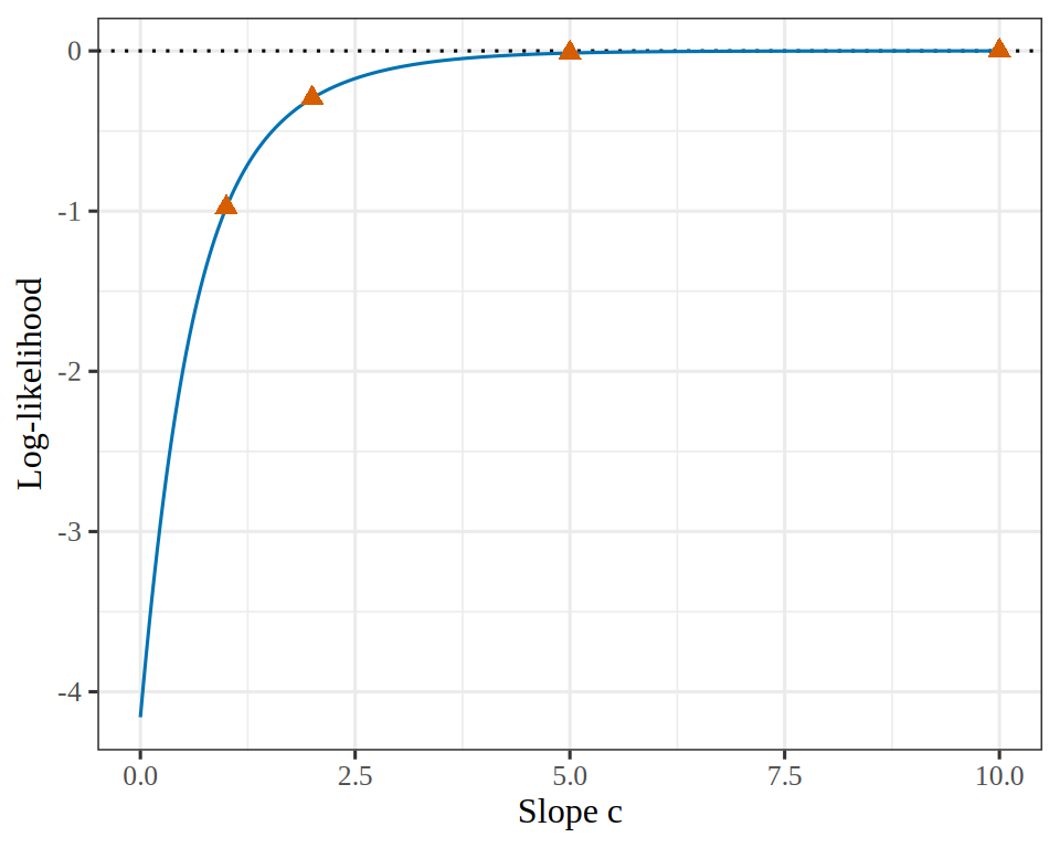
Example 6 (The likelihood keeps rising along a ray)
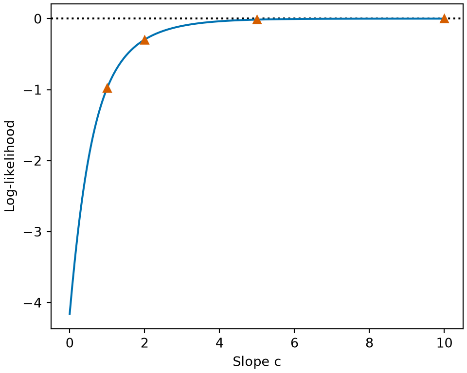
Example 6 (The likelihood keeps rising along a ray) Consider the six patients of Exercise 9, with doses \(-3, -2, -1, 1, 2, 3\) and recoveries \(0, 0, 0, 1, 1, 1\). The vector \(\vcoef = \tp{(0, 1)}\) separates them (Example 1). Scale it by \(c = 1, 2, 5, 10\), which gives \(\coef{0} = 0\) and \(\coef{1} = c\).
As Theorem 1 states, the log-likelihood increases with \(c\), from -0.978 at \(c = 1\) to -9.08e-05 at \(c = 10\). It approaches its supremum \(0\) and does not reach it, so the likelihood approaches its supremum \(1\) and does not reach it either.
Figure 5 plots the curve against \(c\).
library(ggplot2)
sep_grid <- data.frame(c = seq(0, 10, length.out = 300))
sep_grid$loglik <- vapply(sep_grid$c, sp_llik, numeric(1))
sep_marks <- data.frame(c = sp_c, loglik = vapply(sp_c, sp_llik, numeric(1)))
ggplot(sep_grid) +
aes(c, loglik) +
geom_hline(yintercept = 0, linetype = "dotted") +
geom_line(colour = "#0072B2") +
geom_point(data = sep_marks, colour = "#D55E00", shape = 17, size = 2.5) +
labs(x = "Slope c", y = "Log-likelihood")import matplotlib.pyplot as plt
import numpy as np
x_sep = np.array([-3, -2, -1, 1, 2, 3])
y_sep = np.array([0, 0, 0, 1, 1, 1])
def llik_sep(b1):
p = 1 / (1 + np.exp(-b1 * x_sep))
return np.sum(y_sep * np.log(p) + (1 - y_sep) * np.log(1 - p))
c_sep = np.linspace(0, 10, 300)
marks_sep = np.array([1, 2, 5, 10])
fig, ax = plt.subplots(figsize=(5, 4), layout="constrained")
ax.axhline(0, color="black", linestyle=":");
ax.plot(c_sep, [llik_sep(c) for c in c_sep], color="#0072B2");
ax.plot(marks_sep, [llik_sep(c) for c in marks_sep], color="#D55E00", marker="^", linestyle="");
ax.set_xlabel("Slope c");
ax.set_ylabel("Log-likelihood");
plt.show()Example 7 (Gradient descent on separated data has nowhere to stop)
Example 7 (Gradient descent on separated data has nowhere to stop) Table 2 lists four observations with one feature \(\predvar_i\), so \(\vx_i = \tp{(1, \predvar_i)}\) and \(\vcoef = \tp{(\coef{0}, \coef{1})}\).
| \(i\) | \(\predvar_i\) | \(\outvar_i\) |
|---|---|---|
| 1 | 1 | 0 |
| 2 | 2 | 0 |
| 3 | 4 | 1 |
| 4 | 5 | 1 |
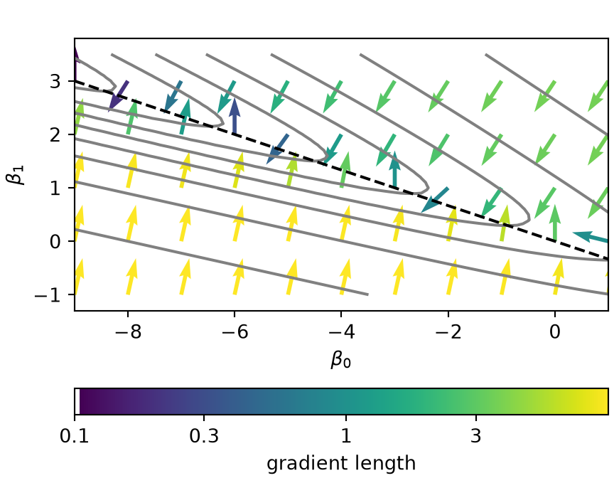
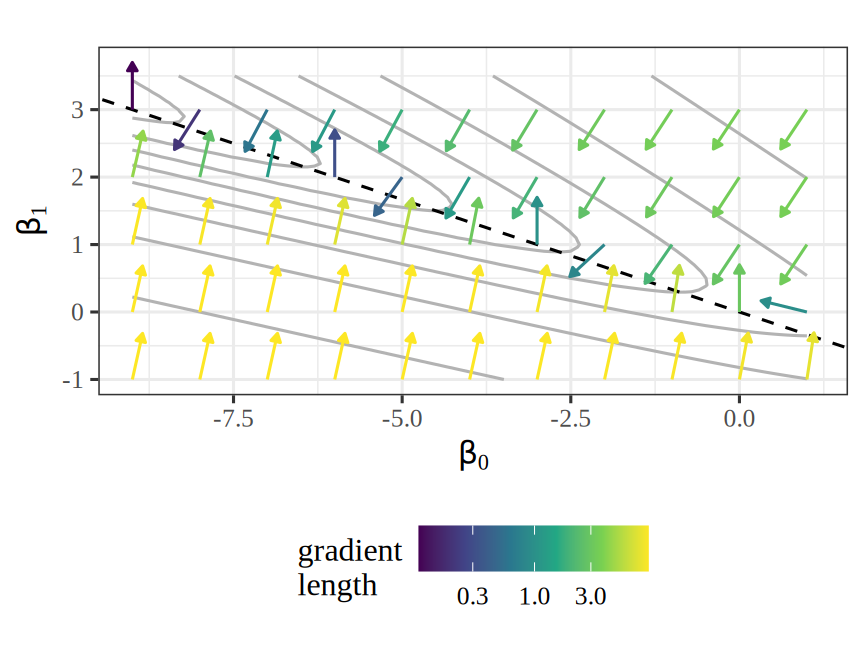
The vector \(\vcoef = \tp{(-3, 1)}\) separates these observations: \(\dprod{\vcoef}{\vx_i} = \predvar_i - 3\) is negative for the two with \(\outvar_i = 0\) and positive for the two with \(\outvar_i = 1\). So, by Theorem 1, the total log loss \(C(\vcoef)\) has no minimizer. The log-likelihood \(\llik = -C\) is concave, so \(C\) is convex, and any point where the gradient \(\grad C(\vcoef)\) is \(\vzero\) would minimize \(C\). No point does, so \(\grad C(\vcoef)\) is never \(\vzero\), and gradient descent never reaches a point where it stops moving.
Figure 6 (a) draws the descent direction \(-\grad C(\vcoef)\) at a grid of points, on the contours of \(C\), and Figure 6 (b) draws the same arrows on its surface. By the logistic gradient theorem, \(\grad C(\vcoef) = \sumin (\prob_i - \outvar_i) \vx_i\), so
\[ \dprod{-\grad C(\vcoef)}{\tp{(-3, 1)}} = \sumin (\prob_i - \outvar_i) (3 - \predvar_i). \]
Each term is positive: an observation with \(\outvar_i = 0\) has \(\prob_i > 0\) and \(\predvar_i < 3\), and one with \(\outvar_i = 1\) has \(\prob_i < 1\) and \(\predvar_i > 3\). So every arrow has a part pointing along the dashed line \(\coef{0} + 3 \coef{1} = 0\) toward the upper left, where \(C\) keeps falling toward 0 without reaching it.
sdd_x <- c(1, 2, 4, 5)
sdd_y <- c(0, 0, 1, 1)
sdd_obs <- tibble::tibble(x = sdd_x, y = sdd_y)
sdd_cost_grad <- tidyr::expand_grid(i = 0:100, j = 0:45) |>
dplyr::mutate(
b0 = -9 + i / 10,
b1 = -1 + j / 10,
on_arrow_grid = i %% 10 == 0 & j %% 10 == 0
) |>
dplyr::cross_join(sdd_obs) |>
dplyr::mutate(
z = b0 + b1 * x,
resid = plogis(z) - y,
loss = -plogis(-z, log.p = TRUE) - y * z
) |>
dplyr::summarise(
cost = sum(loss),
d0 = sum(resid),
d1 = sum(resid * x),
.by = c(b0, b1, on_arrow_grid)
)
sdd_cost_range <- range(sdd_cost_grad$cost)
sdd_len <- 0.7
sdd_arrows <- sdd_cost_grad |>
dplyr::filter(on_arrow_grid) |>
dplyr::mutate(
grad_norm = sqrt(d0^2 + d1^2),
b0_end = b0 - sdd_len * d0 / grad_norm,
b1_end = b1 - sdd_len * d1 / grad_norm
)
sdd_head_size <- grid::unit(0.05, "inches")
sdd_head <- grid::arrow(length = sdd_head_size, type = "closed")
sdd_arrow_aes <- ggplot2::aes(
x = b0, y = b1, xend = b0_end, yend = b1_end, colour = grad_norm
)
# Contours at values of C that double from 1/8 to 16 (see the text).
sdd_levels <- 2^(-3:4)
sdd_xlab <- expression(beta[0])
sdd_ylab <- expression(beta[1])
sdd_plot <- sdd_cost_grad |>
ggplot2::ggplot() +
ggplot2::aes(x = b0, y = b1, z = cost) +
ggplot2::geom_contour(
breaks = sdd_levels, # check-unexplained-choices: allow
colour = "grey70"
) +
ggplot2::geom_abline(intercept = 0, slope = -1 / 3, linetype = "dashed") +
ggplot2::geom_segment(
data = sdd_arrows,
mapping = sdd_arrow_aes,
inherit.aes = FALSE,
arrow = sdd_head
) +
ggplot2::scale_colour_viridis_c(transform = "log10") +
ggplot2::coord_equal() +
ggplot2::labs(x = sdd_xlab, y = sdd_ylab, colour = "gradient\nlength") +
ggplot2::theme(legend.position = "bottom")
# The arrows' colours, reused by the surface.
sdd_layer <- ggplot2::layer_data(sdd_plot, 3)
sdd_arrows$colour <- sdd_layer$colour
sdd_plotimport matplotlib.pyplot as plt
import numpy as np
from matplotlib.colors import LogNorm
x_obs = np.array([1, 2, 4, 5])
y_obs = np.array([0, 0, 1, 1])
def cost_and_grad(b0, b1):
z = b0[..., None] + b1[..., None] * x_obs
resid = 1 / (1 + np.exp(-z)) - y_obs
cost = (np.logaddexp(0, z) - y_obs * z).sum(axis=-1)
return cost, resid.sum(axis=-1), (resid * x_obs).sum(axis=-1)
b0, b1 = np.meshgrid(np.linspace(-9, 1, 101), np.linspace(-1, 3.5, 46))
cost, _, _ = cost_and_grad(b0, b1)
a0, a1 = np.meshgrid(np.arange(-9, 2), np.arange(-1, 4))
_, d0, d1 = cost_and_grad(a0.astype(float), a1.astype(float))
norm = np.hypot(d0, d1)
fig, ax = plt.subplots(figsize=(4.5, 3.5), layout="constrained")
# Contours at values of C that double from 1/8 to 16 (see the text).
ax.contour(b0, b1, cost, levels=2.0 ** np.arange(-3, 5), colors="grey");
ax.axline((0, 0), slope=-1 / 3, color="black", linestyle="--");
arrows = ax.quiver(a0, a1, -d0 / norm, -d1 / norm, norm, norm=LogNorm(),
cmap="viridis", angles="xy", scale_units="xy", scale=1 / 0.7)
bar = fig.colorbar(arrows, ax=ax, location="bottom", label="gradient length")
bar.set_ticks([0.1, 0.3, 1, 3], labels=["0.1", "0.3", "1", "3"]);
bar.minorticks_off();
# Room for the arrows on the top and bottom rows.
ax.set_ylim(-1.3, 3.8);
ax.set_aspect("equal");
ax.set_xlabel(r"$\beta_0$");
ax.set_ylabel(r"$\beta_1$");
plt.show()sdd_grey_low <- c(0, "#e5e5e5")
sdd_grey_high <- c(1, "#808080")
sdd_grey <- list(sdd_grey_low, sdd_grey_high)
sdd_eye <- list(x = -1.4, y = -1.8, z = 1)
sdd_camera <- list(eye = sdd_eye)
sdd_beta <- intToUtf8(946)
sdd_xtitle <- paste0(sdd_beta, "<sub>0</sub>")
sdd_ytitle <- paste0(sdd_beta, "<sub>1</sub>")
sdd_xaxis <- list(title = sdd_xtitle)
sdd_yaxis <- list(title = sdd_ytitle)
sdd_zaxis <- list(title = "C")
sdd_scene <- list(
xaxis = sdd_xaxis,
yaxis = sdd_yaxis,
zaxis = sdd_zaxis,
aspectmode = "cube",
camera = sdd_camera
)
sdd_widget <- plotly::plot_ly() |>
plotly::add_surface(
x = sdd_b0,
y = sdd_b1,
z = sdd_z,
colorscale = sdd_grey,
showscale = FALSE,
opacity = 0.8
)
# One trace per arrow: a shaft, and a marker at the tip.
sdd_n_arrows <- nrow(sdd_arrows)
for (k in seq_len(sdd_n_arrows)) {
sdd_k <- sdd_arrows[k, ]
sdd_line <- list(color = sdd_k$colour, width = 5)
sdd_tip <- list(color = sdd_k$colour, size = 3)
sdd_xs <- c(sdd_k$b0, sdd_k$b0_end)
sdd_ys <- c(sdd_k$b1, sdd_k$b1_end)
sdd_zs <- c(sdd_k$cost, sdd_k$cost_end)
sdd_widget <- sdd_widget |>
plotly::add_paths(
x = sdd_xs, y = sdd_ys, z = sdd_zs, line = sdd_line,
showlegend = FALSE, hoverinfo = "skip"
) |>
plotly::add_markers(
x = sdd_k$b0_end, y = sdd_k$b1_end, z = sdd_k$cost_end,
marker = sdd_tip, showlegend = FALSE, hoverinfo = "skip"
)
}
sdd_widget <- plotly::layout(sdd_widget, scene = sdd_scene)
htmltools::div(role = "img", `aria-label` = sdd_alt, sdd_widget)import html
import matplotlib as mpl
import plotly.graph_objects as go
ends0, ends1 = a0 - 0.7 * d0 / norm, a1 - 0.7 * d1 / norm
start_cost, _, _ = cost_and_grad(a0.astype(float), a1.astype(float))
end_cost = start_cost - 0.7 * norm # in the tangent plane at the start
colours = mpl.colormaps["viridis"](LogNorm()(norm))
fig = go.Figure(go.Surface(x=b0[0], y=b1[:, 0], z=cost, showscale=False,
opacity=0.8,
colorscale=[[0, "#e5e5e5"], [1, "#808080"]]))
for k in np.ndindex(norm.shape):
colour = mpl.colors.to_hex(colours[k])
fig.add_trace(go.Scatter3d(
x=[a0[k], ends0[k]], y=[a1[k], ends1[k]], z=[start_cost[k], end_cost[k]],
mode="lines", line=dict(color=colour, width=5), showlegend=False,
hoverinfo="skip"));
fig.add_trace(go.Scatter3d(
x=[ends0[k]], y=[ends1[k]], z=[end_cost[k]], mode="markers",
marker=dict(color=colour, size=3), showlegend=False,
hoverinfo="skip"));
beta = chr(946) # Greek beta, as a code point to keep the source ASCII
fig.update_layout(scene=dict(xaxis_title=beta + "<sub>0</sub>",
yaxis_title=beta + "<sub>1</sub>",
zaxis_title="C", aspectmode="cube",
camera=dict(eye=dict(x=-1.4, y=-1.8, z=1))));
print("```{=html}\n"
+ f'<div role="img" aria-label="{html.escape(r.sdd_alt)}">\n'
+ fig.to_html(full_html=False, include_plotlyjs="cdn") + "\n</div>\n```")Remark 2 (Why the contour levels double)
Remark 2 (Why the contour levels double). The contours in Figure 6 (a) are drawn at values of \(C\) that double from 1/8 to 16, because over the plotted window \(C\) runs from 0.096, slightly above the dashed line at the upper left, to 27, at the lower left. Evenly spaced levels would crowd into the lower left and leave none where the arrows head.
Example 8 (The zero curves of the two partial derivatives never meet)
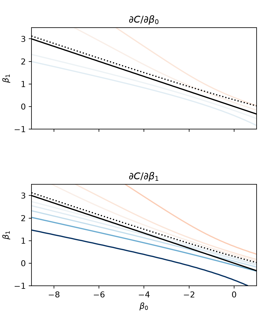
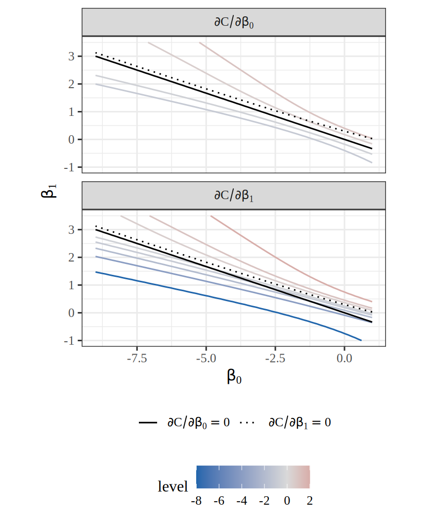
Example 8 (The zero curves of the two partial derivatives never meet) For the four observations of Table 2, the gradient \(\grad C(\vcoef)\) of the total log loss is \(\vzero\) only where both partial derivatives are 0, so such a point would lie on the zero curve of each. Example 7 showed that
\[ 3 \derivf{C}{\coef{0}} - \derivf{C}{\coef{1}} = \sumin (\prob_i - \outvar_i) (3 - \predvar_i) > 0 \]
for every \(\vcoef\). So wherever \(\derivf{C}{\coef{0}} = 0\), \(\derivf{C}{\coef{1}}\) is negative, and the two zero curves never meet.
Figure 7 (a) draws each partial derivative as level curves and Figure 7 (b) as a surface, with both zero curves in every panel. The zero curve of \(\derivf{C}{\coef{0}}\) (solid) is the line \(\coef{0} + 3 \coef{1} = 0\), because \(\derivf{C}{\coef{0}} = \sumin (\prob_i - \outvar_i)\) and on that line the four predicted probabilities are \(\expitf{-2 \coef{1}}\), \(\expitf{-\coef{1}}\), \(\expitf{\coef{1}}\) and \(\expitf{2 \coef{1}}\), which pair up as \(\expitf{-t} + \expitf{t} = 1\) and so add up to 2, the number of observations with \(\outvar_i = 1\). Off the line, \(\derivf{C}{\coef{0}}\) is not 0, because it increases with \(\coef{0}\) for each fixed \(\coef{1}\). The zero curve of \(\derivf{C}{\coef{1}}\) (dotted) lies above the solid curve: on the solid curve \(\derivf{C}{\coef{1}}\) is negative, for the reason given at the start of this example, and \(\derivf{C}{\coef{1}}\) increases with \(\coef{1}\) for each fixed \(\coef{0}\), because the partial derivative of \(\derivf{C}{\coef{1}}\) in \(\coef{1}\) is \(\sumin \prob_i (1 - \prob_i) \predvar_i^2 > 0\).
spd_long <- sdd_cost_grad |>
dplyr::select(b0, b1, d0, d1) |>
tidyr::pivot_longer(
cols = dplyr::starts_with("d"),
names_to = "partial",
values_to = "value"
) |>
dplyr::mutate(
panel = dplyr::if_else(
partial == "d0",
"partialdiff * C / partialdiff * beta[0]",
"partialdiff * C / partialdiff * beta[1]"
)
)
# Level curves at these values of each partial derivative (see the text).
spd_levels <- c(-8, -4, -2, -1, -0.5, 0.5, 1, 2)
spd_level_aes <- ggplot2::aes(colour = ggplot2::after_stat(level))
spd_zero0_aes <- ggplot2::aes(x = b0, y = b1, z = d0, linetype = "d0")
spd_zero1_aes <- ggplot2::aes(x = b0, y = b1, z = d1, linetype = "d1")
spd_zero_labels <- expression(
partialdiff * C / partialdiff * beta[0] == 0,
partialdiff * C / partialdiff * beta[1] == 0
)
spd_zero_types <- c(d0 = "solid", d1 = "dotted")
spd_panel <- ggplot2::vars(panel)
spd_plot <- spd_long |>
ggplot2::ggplot() +
ggplot2::aes(x = b0, y = b1, z = value) +
ggplot2::geom_contour(
mapping = spd_level_aes,
breaks = spd_levels # check-unexplained-choices: allow
) +
ggplot2::geom_contour(
data = sdd_cost_grad, mapping = spd_zero0_aes,
breaks = 0, colour = "black" # check-unexplained-choices: allow
) +
ggplot2::geom_contour(
data = sdd_cost_grad, mapping = spd_zero1_aes,
breaks = 0, colour = "black" # check-unexplained-choices: allow
) +
ggplot2::facet_wrap(spd_panel, ncol = 1, labeller = ggplot2::label_parsed) +
ggplot2::scale_colour_gradient2(
low = "#2166ac", mid = "grey85", high = "#b2182b", midpoint = 0
) +
ggplot2::scale_linetype_manual(
values = spd_zero_types, labels = spd_zero_labels
) +
ggplot2::coord_equal() +
ggplot2::labs(
x = sdd_xlab, y = sdd_ylab, colour = "level", linetype = NULL
) +
ggplot2::theme(legend.position = "bottom", legend.box = "vertical")
spd_plot_, d0_grid, d1_grid = cost_and_grad(b0, b1)
# Level curves at these values of each partial derivative (see the text).
levels = [-8, -4, -2, -1, -0.5, 0.5, 1, 2]
fig, axes = plt.subplots(2, 1, figsize=(4.5, 5.5), layout="constrained",
sharex=True)
for ax, z, name in zip(axes, [d0_grid, d1_grid], ["0", "1"]):
ax.contour(b0, b1, z, levels=levels, cmap="RdBu_r", vmin=-8, vmax=8);
ax.contour(b0, b1, d0_grid, levels=[0], colors="black");
ax.contour(b0, b1, d1_grid, levels=[0], colors="black",
linestyles="dotted");
ax.set_aspect("equal");
ax.set_title(rf"$\partial C / \partial \beta_{name}$");
ax.set_ylabel(r"$\beta_1$");
axes[1].set_xlabel(r"$\beta_0$");
plt.show()spd_alt <- paste(
"Two interactive 3D surfaces over the plane of the intercept and the",
"slope: the partial derivatives of the total log loss in the intercept",
"and in the slope, red where positive and blue where negative.",
"Each crosses height 0 along its own black zero curve,",
"solid for the intercept and dotted for the slope,",
"and the two curves never meet. Buttons show one surface at a time."
)
spd_scale_low <- c(0, "#2166ac")
spd_scale_mid <- c(0.5, "#d9d9d9")
spd_scale_high <- c(1, "#b2182b")
spd_scale <- list(spd_scale_low, spd_scale_mid, spd_scale_high)
spd_names <- c("dC/d(beta 0)", "dC/d(beta 1)")
spd_surfaces <- list(spd_d0, spd_d1)
spd_widget <- plotly::plot_ly()
for (k in 1:2) {
spd_widget <- spd_widget |>
plotly::add_surface(
x = sdd_b0, y = sdd_b1, z = spd_surfaces[[k]], name = spd_names[k],
colorscale = spd_scale, cmin = -8, cmax = 8, showscale = FALSE,
opacity = 0.85
)
}
spd_dashes <- c("solid", "dot")
for (k in 1:2) {
spd_line <- list(color = "black", width = 5, dash = spd_dashes[k])
for (piece in spd_zero_sets[[k]]) {
spd_widget <- spd_widget |>
plotly::add_paths(
x = piece$x, y = piece$y, z = 0 * piece$x, line = spd_line,
showlegend = FALSE, hoverinfo = "skip"
)
}
}
# Buttons show both surfaces or one; the zero curves stay visible.
spd_built <- plotly::plotly_build(spd_widget)
spd_n_traces <- length(spd_built$x$data)
spd_curves <- rep(TRUE, spd_n_traces - 2)
spd_show_both <- c(TRUE, TRUE)
spd_show_d0 <- c(TRUE, FALSE)
spd_show_d1 <- c(FALSE, TRUE)
spd_show <- list(spd_show_both, spd_show_d0, spd_show_d1)
spd_labels <- c("both", spd_names)
spd_buttons <- list()
for (k in 1:3) {
spd_shown <- spd_show[[k]]
spd_visible <- c(spd_shown, spd_curves)
spd_restyle <- list(visible = spd_visible)
spd_args <- list(spd_restyle)
spd_buttons[[k]] <- list(
method = "restyle", args = spd_args, label = spd_labels[k]
)
}
spd_menu <- list(type = "buttons", direction = "right", buttons = spd_buttons)
spd_menus <- list(spd_menu)
spd_zaxis <- list(title = "partial derivative")
spd_scene <- list(
xaxis = sdd_xaxis, yaxis = sdd_yaxis, zaxis = spd_zaxis,
aspectmode = "cube", camera = sdd_camera
)
spd_widget <- plotly::layout(
spd_widget, scene = spd_scene, updatemenus = spd_menus
)
htmltools::div(role = "img", `aria-label` = spd_alt, spd_widget)scale = [[0, "#2166ac"], [0.5, "#d9d9d9"], [1, "#b2182b"]]
fig = go.Figure()
for z, name in [(d0_grid, "dC/d(beta 0)"), (d1_grid, "dC/d(beta 1)")]:
fig.add_trace(go.Surface(x=b0[0], y=b1[:, 0], z=z, name=name,
colorscale=scale, cmin=-8, cmax=8,
showscale=False, opacity=0.85));
for z, dash in [(d0_grid, "solid"), (d1_grid, "dot")]:
zero = plt.contour(b0, b1, z, levels=[0])
for path in zero.allsegs[0]:
fig.add_trace(go.Scatter3d(x=path[:, 0], y=path[:, 1], z=0 * path[:, 0],
mode="lines", showlegend=False,
line=dict(color="black", width=5, dash=dash)));
plt.close()
curves = [True] * (len(fig.data) - 2)
buttons = [dict(method="restyle", label=label, args=[{"visible": show + curves}])
for label, show in [("both", [True, True]),
("dC/d(beta 0)", [True, False]),
("dC/d(beta 1)", [False, True])]]
fig.update_layout(
updatemenus=[dict(type="buttons", direction="right", buttons=buttons)],
scene=dict(xaxis_title=beta + "<sub>0</sub>",
yaxis_title=beta + "<sub>1</sub>",
zaxis_title="partial derivative", aspectmode="cube",
camera=dict(eye=dict(x=-1.4, y=-1.8, z=1))));
print("```{=html}\n"
+ f'<div role="img" aria-label="{html.escape(r.spd_alt)}">\n'
+ fig.to_html(full_html=False, include_plotlyjs="cdn") + "\n</div>\n```")Remark 3 (Why these level curves)
Remark 3 (Why these level curves). The level curves in Figure 7 (a) are drawn at \(\pm 0.5\), \(\pm 1\), \(\pm 2\), \(-4\) and \(-8\), because over the plotted window \(\derivf{C}{\coef{0}}\) runs from -2 to 2 and \(\derivf{C}{\coef{1}}\) from -9 to 3. Levels that double away from 0 cover both of them with the same colors, and leave room near 0 for the zero curves.
library(ggplot2)
set.seed(571)
n_per_class <- 15
sim_df <- data.frame(
x1 = c(rnorm(n_per_class, -2.5, 0.6), rnorm(n_per_class, 2.5, 0.6)),
x2 = rnorm(2 * n_per_class, 0, 0.9),
class = rep(c("Left", "Right"), each = n_per_class)
)
# Each boundary passes through the midpoint of the class means,
# at a different angle (in degrees) from the horizontal axis.
pivot <- c(mean(sim_df$x1), mean(sim_df$x2))
angles <- c(f1 = 55, f2 = 90, f3 = 125)
boundary_df <- data.frame(
boundary = paste(names(angles), "= 0"),
angle = angles * pi / 180
)
# Check that every boundary separates the two classes.
side <- function(angle) {
(sim_df$x1 - pivot[1]) * sin(angle) - (sim_df$x2 - pivot[2]) * cos(angle) > 0
}
stopifnot(all(vapply(
boundary_df$angle,
function(a) nrow(unique(data.frame(side(a), sim_df$class))) == 2,
logical(1)
)))
# geom_abline cannot draw a vertical line, so draw each boundary as a segment.
boundary_df$x_start <- pivot[1] - 10 * cos(boundary_df$angle)
boundary_df$x_end <- pivot[1] + 10 * cos(boundary_df$angle)
boundary_df$y_start <- pivot[2] - 10 * sin(boundary_df$angle)
boundary_df$y_end <- pivot[2] + 10 * sin(boundary_df$angle)
ggplot(sim_df) +
aes(x1, x2) +
geom_point(aes(colour = class, shape = class), size = 2.5) +
geom_segment(
data = boundary_df,
aes(x = x_start, y = y_start, xend = x_end, yend = y_end, linetype = boundary)
) +
scale_colour_manual(values = c(Left = "#D55E00", Right = "#0072B2")) +
scale_shape_manual(values = c(Left = 3, Right = 16)) +
scale_linetype_manual(values = c(
"f1 = 0" = "solid", "f2 = 0" = "dashed", "f3 = 0" = "dotted"
)) +
coord_cartesian(xlim = range(sim_df$x1), ylim = range(sim_df$x2)) +
labs(x = "Feature 1, x1", y = "Feature 2, x2", colour = NULL, shape = NULL, linetype = NULL)import matplotlib.pyplot as plt
import numpy as np
rng = np.random.default_rng(571)
n_per_class = 15
left = np.column_stack([rng.normal(-2.5, 0.6, n_per_class),
rng.normal(0, 0.9, n_per_class)])
right = np.column_stack([rng.normal(2.5, 0.6, n_per_class),
rng.normal(0, 0.9, n_per_class)])
points = np.vstack([left, right])
is_right = np.repeat([False, True], n_per_class)
# Each boundary passes through the midpoint of the class means,
# at a different angle (in degrees) from the horizontal axis.
pivot = points.mean(axis=0)
angles = {"f1": 55, "f2": 90, "f3": 125}
styles = {"f1": "-", "f2": "--", "f3": ":"}
def side(angle):
offset = points - pivot
return offset[:, 0] * np.sin(angle) - offset[:, 1] * np.cos(angle) > 0
# Check that every boundary separates the two classes.
for degrees in angles.values():
assert len(set(zip(side(np.radians(degrees)), is_right))) == 2
fig, ax = plt.subplots(figsize=(5, 3.6), layout="constrained")
ax.scatter(*left.T, marker="+", color="#D55E00", label="Left");
ax.scatter(*right.T, marker="o", color="#0072B2", label="Right");
x_lim, y_lim = ax.get_xlim(), ax.get_ylim()
for name, degrees in angles.items():
direction = np.array([np.cos(np.radians(degrees)), np.sin(np.radians(degrees))])
ends = pivot + np.outer([-10, 10], direction)
ax.plot(*ends.T, styles[name], color="black", label=f"{name} = 0");
ax.set_xlim(x_lim);
ax.set_ylim(y_lim);
ax.set_xlabel("Feature 1, x1");
ax.set_ylabel("Feature 2, x2");
fig.legend(loc="outside lower center", ncol=5, frameon=False);
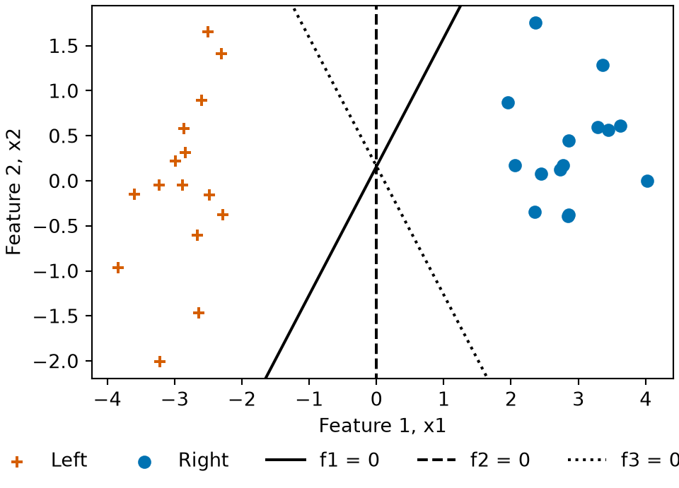
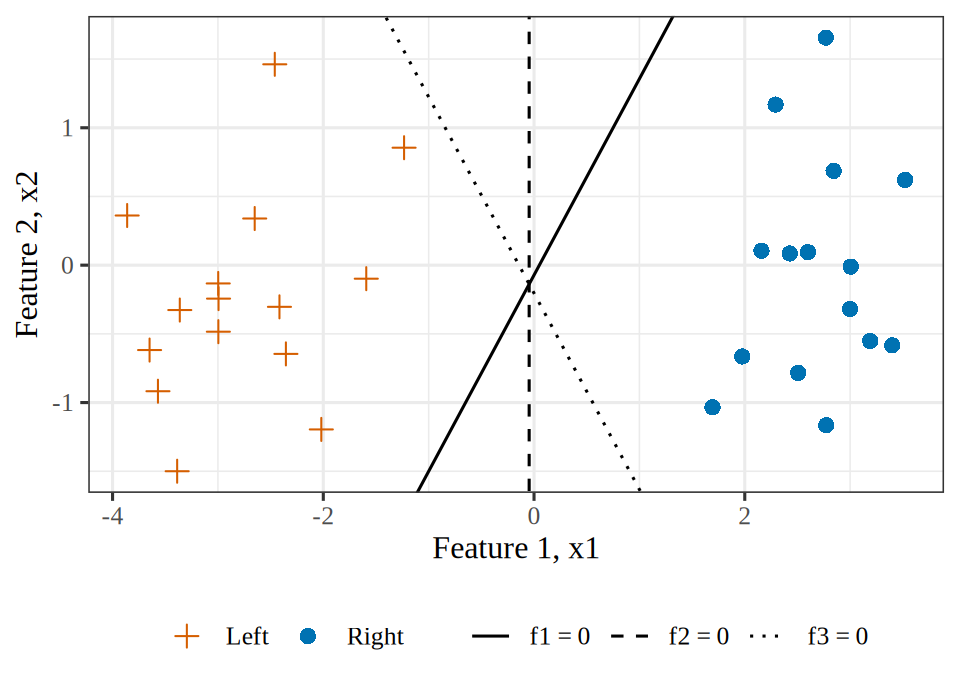
plt.show()Every boundary in Figure 8 classifies the simulated points without error, and the one farthest from the nearest point of either class has the largest margin. Maximizing the logistic likelihood does not give that boundary. The log loss of an observation, \(\log\paren{1 + \e{-m}}\), decreases exponentially in its margin \(m = \signoutvar \dprod{\vcoef}{\vx}\) and never reaches \(0\), so on separated data the likelihood keeps increasing as \(\norm{\vcoef}\) grows along a separating direction, and there is no finite maximizer (Theorem 1). A ridge penalty gives a finite maximizer (Solution 22). As the penalty weight tends to \(0\), the direction of the penalized fit approaches that of the maximum-margin boundary [6]. Support vector machines maximize the margin of the separating hyperplane directly, and their solution is finite.
The six patients of Exercise 9 were made up so the algebra could be done by hand. Separation also turns up in published studies, and fitting software reports it no more clearly there.
Dataset 2: The endometrial cancer data
Heinze and Schemper analyzed endometrial cancer data on 79 patients as an example of separation [7]. Asseryanis, of the Medical University of Vienna, provided the data. The copy here comes from the endometrial table in the R package brglm2. The data are in data/endometrial.csv, one patient per line:
HG: the outcome, the histology grade of the tumor, 1 for high grade and 0 for low grade.NV: neovascularization, 1 if new blood vessels have formed in the tumor and 0 if not.PI: the pulsatility index of the uterine artery.EH: the height of the endometrium.Exercise 25 (Separation in the endometrial cancer data: what software reports)
Exercise 25 (Separation in the endometrial cancer data: what software reports) Data from published studies can be quasi-completely separated too. In the endometrial cancer data, tabulating the histology grade HG against neovascularization NV shows that every patient with NV \(= 1\) has a high-grade tumor:
# Read the local copy, then count the patients in each NV and HG cell,
# listing the empty cell with a count of 0 rather than dropping it.
endo <- readr::read_csv("data/endometrial.csv", show_col_types = FALSE)
empty_cell_count <- list(n = 0L)
endo |>
dplyr::count(NV, HG) |>
tidyr::complete(NV, HG, fill = empty_cell_count)Fit the logistic regression of HG on NV with R’s glm(). What does it report?
Hint
Compare the report with the quasi-completely separated example of Example 2.
Solution 25. Fitting the endometrial cancer data with R’s glm():
# Fit HG on NV, then tabulate the coefficients with parameters.
endo_fit <- glm(HG ~ NV, family = binomial, data = endo)
endo_coefs <- summary(endo_fit)$coefficients
endo_b1_hat <- coef(endo_fit)[["NV"]]
endo_se_hat <- endo_coefs["NV", "Std. Error"]
endo_p_hat <- endo_coefs["NV", "Pr(>|z|)"]
parameters::parameters(endo_fit) |> parameters::print_md(digits = 3)| Parameter | Log-Odds | SE | 95% CI | z | p |
|---|---|---|---|---|---|
| (Intercept) | -1.059 | 0.281 | (-1.639, -0.528) | -3.761 | < .001 |
| NV | 19.625 | 1809.054 | (-104.915, ) | 0.011 | 0.991 |
R reports a slope of 19.6 for NV, with a standard error of 1809 and a \(p\)-value of 0.991. It gives no warning. An odds ratio of \(\expf{19.6}\) is not a plausible value for any predictor.
NV quasi-completely separates the data. The 13 patients with NV \(= 1\) all have HG \(= 1\), while the 66 patients with NV \(= 0\) include both grades. So the maximum likelihood estimate of the slope does not exist [4], [7], and the only sign of trouble in the output is the large standard error.
Exercise 26 (Separation in the endometrial cancer data: why the fit stops)
Exercise 26 (Separation in the endometrial cancer data: why the fit stops) R’s glm() reports a slope for NV when it fits the logistic regression of the histology grade HG on NV in the endometrial cancer data (Solution 25).
Why does glm() stop at that slope?
Hint
Compare the stopped fit for the six patients of Exercise 9 in Example 4.
Solution 26. The log-likelihood of the endometrial cancer data keeps increasing as the slope of NV grows. Each increase moves the fitted probability for the patients with NV \(= 1\) closer to their observed \(1\). Far out, the log-likelihood changes very little. There the gradient and the change in fit are both small, so a fitting routine stops there, at a slope that its tolerance determines, without having found a maximum. glm() stops after 17 iterations, when the relative change in the deviance falls below its tolerance, epsilon = 1e-8 by default. The reported slope \(19.62\) depends on that tolerance; it is not an estimate of a finite parameter. Running the same fit with a tighter tolerance:
slope iterations
32.62489 30.00000
returns a larger slope, \(32.62\), after 30 iterations. Only this fit makes R warn, “fitted probabilities numerically 0 or 1 occurred”. At the default tolerance the fit stopped before any fitted probability rounded to \(1\).
Exercise 27 (Separation in the endometrial cancer data: the likelihood ratio test)
Exercise 27 (Separation in the endometrial cancer data: the likelihood ratio test) R’s glm() gives the slope of NV a Wald test \(p\)-value of 0.991 in the logistic regression of the histology grade HG on NV in the endometrial cancer data (Solution 25).
Compute the likelihood ratio statistic \(G^2\) for \(H_0\): the slope of NV is \(0\), and its \(p\)-value from the \(\chi^2_1\) distribution.
Hint
\(G^2\) is the null deviance minus the deviance of the fit, as in Solution 19. In R, anova() with test = "LRT" compares two nested fits.
Solution 27. Under \(H_0\) the slope of NV is \(0\), so the null fit has an intercept alone. The unrestricted fit has no maximizer, so the log-likelihood at the slope where glm() stopped takes the place of the maximized log-likelihood in the likelihood ratio statistic. That log-likelihood is less than \(10^{-6}\) below its supremum, because the log-likelihood changes very little that far out (Solution 26). Comparing the two fits of the endometrial cancer data:
\(G^2\) is the null deviance minus the deviance of the fit:
\[ \begin{aligned} G^2 &= 104.9 - 75.31 \\ &= 29.6. \end{aligned} \]
Against the \(\chi^2_1\) distribution, \(G^2\) gives \(p = 5.3\times 10^{-8}\), while the Wald test of the same hypothesis gave \(p = 0.991\).
Exercise 28 (Separation in the endometrial cancer data: which test to use)
Exercise 28 (Separation in the endometrial cancer data: which test to use) For the slope of NV in the logistic regression of the histology grade HG on NV in the endometrial cancer data, the Wald test gives \(p = 0.991\) (Solution 25) and the likelihood ratio test gives \(p = 5.3\times 10^{-8}\) (Solution 27).
Which of the two should you use here?
Hint
Look again at the Hauck–Donner effect.
Solution 28. Use the likelihood ratio test: it finds a strong association between NV and the histology grade HG. The Wald statistic is the slope divided by its standard error, and glm() stopped where both are large and the standard error has grown faster than the slope, so the Wald statistic is near \(0\). That decrease is the Hauck–Donner effect. The Wald test uses the curvature of the log-likelihood at the fitted slope, far out, where the log-likelihood changes very little. The likelihood ratio test uses the change in log-likelihood between a slope of \(0\) and the fit, which shows how much better the quasi-completely separated fit describes the endometrial cancer data.
Exercise 29 (Separation in the endometrial cancer data: how far to trust the p-value)
Exercise 29 (Separation in the endometrial cancer data: how far to trust the p-value) For the slope of NV in the logistic regression of the histology grade HG on NV in the endometrial cancer data, the likelihood ratio test \(p\)-value of Solution 27 relies on the \(\chi^2_1\) approximation. Only 13 patients have NV \(= 1\).
Compute a \(p\)-value that needs no approximation, by conditioning on the number of high-grade tumors.
Hint
With one binary predictor, conditioning on the number of patients with NV \(= 1\) as well as the number of high-grade tumors gives Fisher’s exact test, fisher.test() in R. Compare the six patients’ test in Solution 21.
Solution 29. The endometrial cancer data have 30 high-grade tumors among 79 patients. Under \(H_0\), given that count and the 13 patients with NV \(= 1\), each way to choose which patients have high-grade tumors is equally likely. The \(p\)-value is the probability of a table at least as extreme as the observed one, which is what Fisher’s exact test computes:
[1] 4.537619e-07
The two-sided \(p\)-value from fisher.test() is \(4.5\times 10^{-7}\). It is larger than the \(\chi^2_1\) value of Solution 27, \(5.3\times 10^{-8}\), but both reject \(H_0\) at any usual level, while the Wald test gave 0.991.
Exercise 30 (Separation in the endometrial cancer data: the penalized slope)
Exercise 30 (Separation in the endometrial cancer data: the penalized slope) In the logistic regression of the histology grade HG on NV in the endometrial cancer data, let \(\coef{0}\) be the intercept, \(\coef{1}\) the slope of NV, and \(\llik(\coef{0}, \coef{1})\) the log-likelihood. The ridge-penalized log-likelihood penalizes the slope alone:
\[ f(\coef{0}, \coef{1}) = \llik(\coef{0}, \coef{1}) - \tfrac{\regpar}{2}\coef{1}^2. \]
Find the slope \(\hcoef{1}\) of the maximizer of \(f\) for \(\regpar = 1\), \(0.1\) and \(0.01\).
Hint
Maximize \(f\) numerically, for example with R’s optim() on \(-f\). Compare the six patients’ penalized slopes in Solution 23.
Solution 30. Maximizing \(f\) numerically for the endometrial cancer data, from a start at \(\coef{0} = \coef{1} = 0\):
# Minus the ridge-penalized log-likelihood.
# The penalty leaves the intercept free.
endo_neg_pen <- function(b, lambda, data) { # nolint: function_location_linter
eta <- b[[1]] + b[[2]] * data$NV
p <- plogis(eta)
loglik_i <- dbinom(data$HG, size = 1, prob = p, log = TRUE)
loglik <- sum(loglik_i)
lambda / 2 * b[[2]]^2 - loglik
}
# A tight tolerance, so the reported slopes do not depend on optim's default.
endo_optim_control <- list(reltol = 1e-14)
endo_ridge_slope <- function(lambda, data) { # nolint: function_location_linter
start <- c(0, 0)
fit <- optim(
start, endo_neg_pen,
lambda = lambda, data = data,
method = "BFGS", control = endo_optim_control
)
fit$par[[2]]
}
endo_lambda <- c(1, 0.1, 0.01)
endo_ridge <- endo_lambda |> purrr::map_dbl(endo_ridge_slope, data = endo)
endo_ridge_cols <- c("$\\regpar$", "$\\hcoef{1}$")
tibble::tibble(lambda = endo_lambda, slope = endo_ridge) |>
knitr::kable(
col.names = endo_ridge_cols,
digits = 3,
align = "r"
)| \(\regpar\) | \(\hcoef{1}\) |
|---|---|
| 1.00 | 2.376 |
| 0.10 | 4.380 |
| 0.01 | 6.368 |
The penalized slope is \(2.38\) at \(\regpar = 1\) and grows to \(6.37\) at \(\regpar = 0.01\).
Exercise 31 (Separation in the endometrial cancer data: what the penalty costs)
Exercise 31 (Separation in the endometrial cancer data: what the penalty costs) The ridge-penalized fits of the endometrial cancer data in Solution 30 give a slope for NV at each of \(\regpar = 1\), \(0.1\) and \(0.01\).
What does the penalty achieve, and at what cost?
Hint
Compare the six patients’ answer in Solution 24.
Solution 31. For the endometrial cancer data, the ridge penalty gives \(f\) a maximizer at every \(\regpar > 0\), so the slope for NV is a number that the fit can report.
The cost is that the slope depends on \(\regpar\). It is 2.7 times larger at \(\regpar = 0.01\) than at \(\regpar = 1\), and it keeps growing as \(\regpar \to 0\), because the likelihood alone keeps increasing as the slope grows. The penalty adds a preference for smaller coefficients, not information about NV from the data, and each penalized slope reflects that preference as much as the data. A report of a penalized fit should therefore state \(\regpar\).
What the 79 patients show is not that \(\hcoef{1} = 4.38\). They show that NV quasi-completely separates the histology grades, that a slope of \(0\) is implausible (\(p = 4.5\times 10^{-7}\), Solution 29), and that the data alone cannot say how large the slope is.