rm(list =ls())# delete any data that's already loaded into Rconflicts_prefer(dplyr::filter)ggplot2::theme_set(ggplot2::theme_bw()+# ggplot2::labs(col = "") +ggplot2::theme( legend.position ="bottom", text =ggplot2::element_text(size =12, family ="serif")))knitr::opts_chunk$set(message =FALSE)options(digits =6)panderOptions("big.mark", ",")pander::panderOptions("table.emphasize.rownames", FALSE)pander::panderOptions("table.split.table", Inf)# use the `filter()` function from dplyr() by defaultconflicts_prefer(dplyr::filter)legend_text_size<-9run_graphs<-TRUE
2 Welcome
Welcome to Epidemiology 204: Quantitative Epidemiology III (Statistical Models).
Epi 204 is a course on regression modeling.
3 What you should already know
Warning
Epi 202, Epi 203, and Sta 108 are prerequisites for this course. If you haven’t passed one of these courses, talk to me ASAP.
number of infections per month; number of follow-up visits per patient
Poisson regression
time to event
time from exposure until disease onset; time from onset until recurrence; time from disease onset until disease progression; time from onset until death
pain level (0 to 10 scale); approval rating (0 to 5 stars)
ordinal regression
5 The scientific method and models
As scientists, we attempt to answer factual questions about the world and universe in the past, present, and/or future. In this course, we follow the steps of the scientific method, with a statistical model standing in for the hypothesis:
conceive a question
hypothesize a specific version of that model
propose a study design that would provide data relevant to the model
analyze the data
estimate model parameters
“inference”:
quantify uncertainty
draw conclusions
Regression models are the family of models we use for these steps.
when there’s not enough data to analyze every subgroup of interest individually
especially when subgroups are defined using continuous predictors
6.1 Uses of regression models
Vittinghoff et al. [3, Sec. 1.3] identifies three broad motivations for using multipredictor regression models:
Multipredictor regression can be a powerful tool for addressing three important practical questions. … [These] include prediction, isolating the effect of a single predictor, and understanding multiple predictors.
Prediction: “Multipredictor regression is a powerful and general tool for using multiple measured predictors to make useful predictions for future observations.”
Isolating the Effect of a Single Predictor: “In settings where multiple, related predictors contribute to study outcomes, it will be important to consider multiple predictors even when a single predictor is of interest.” (e.g., to minimize confounding and support causal interpretation)
Understanding Multiple Predictors: “Multipredictor regression can also be used when our aim is to identify multiple independent predictors of a study outcome — independent in the sense that they appear to have an effect over and above other measured variables.” (including mediation and interaction)
Kleinbaum et al. [4, Sec. 4.1] provides a more granular list of eight overlapping applications of regression analysis:
In practice, a regression analysis is appropriate for several possibly overlapping situations, including the following:
Characterize the association: “You want to characterize the relationship between the dependent and independent variables by determining the extent, direction, and strength of the association.”
Prediction: “You seek a quantitative formula or equation to describe (e.g., predict) the dependent variable \(Y\) as a function of the independent variables \(X_1, X_2, \ldots, X_k\).”
Controlled description: “You want to describe quantitatively or qualitatively the relationship between \(X_1, X_2, \ldots, X_k\) and \(Y\) but control for the effects of still other variables \(X_{k+1}, X_{k+2}, \ldots, X_{k+p}\), which you believe have an important relationship with the dependent variable.”
Variable selection: “You want to determine which of several independent variables are important and which are not for describing or predicting a dependent variable. You may want to control for other variables. You may also want to rank independent variables in their order of importance.”
Model selection: “You want to determine the best mathematical model for describing the relationship between a dependent variable and one or more independent variables.”
Comparing regression relationships: “You want to compare several derived regression relationships.” (e.g., whether a relationship between two variables differs across subgroups)
Interaction: “You want to assess the interactive effects of two or more independent variables with regard to a dependent variable.”
Adjusted coefficient estimation: “You want to obtain a valid and precise estimate of one or more regression coefficients from a larger set of regression coefficients in a given model.” (i.e., estimating the effect of one variable after adjusting for others)
6.1.1 Relating the two lists
The two lists use different levels of granularity to describe the same landscape of regression uses. Vittinghoff et al. [3] provides three broad categories, while Kleinbaum et al. [4] identifies eight more specific applications.
Table 2: Comparing the categorizations of regression model uses in Vittinghoff et al. [3, Sec. 1.3] and Kleinbaum et al. [4, Sec. 4.1]
Applications 6 and 7 are related but distinct: Application 6 asks whether a derived regression relationship (e.g., a coefficient or the overall model) differs across pre-defined groups, typically by comparing models fit separately for each group. Application 7 asks whether two predictors interact within a single model — that is, whether the effect of one predictor on the outcome depends on the value of another predictor. In that sense, Application 6 can be viewed as a special case of Application 7 where the grouping variable is the effect modifier.
The key conceptual distinction made by Vittinghoff et al. [3] — but not explicitly highlighted by Kleinbaum et al. [4] — is between prediction (forecasting future outcomes) and causal inference (estimating the effect of a specific predictor). This distinction has important implications for model building strategy: prediction models can include any variables that improve predictive accuracy, while causal inference requires careful consideration of confounding, mediation, and the causal structure of the data.
6.1.2 Prediction, Inference, and Causal Inference
The goal of prediction is to forecast an outcome \(Y\) for new observations, given observed predictor variables \(X_1, \ldots, X_p\). In a prediction problem, the model is often treated as a “black box”: we care about predictive accuracy, not about the exact form or interpretation of the relationship between predictors and outcome [5, Ch. 2].
Example 1 For example, a clinical prediction model might identify which patients are at highest risk of hospital readmission, using demographics, diagnoses, and laboratory values, without requiring that each predictor be causally related to readmission.
At its core, prediction aspires to minimize uncertainty: the goal is that, by including enough informative predictors and combining them flexibly, we can reduce as much as possible the residual randomness in our forecasts.
Statistical inference also studies the relationship between \(Y\) and \(X_1, \ldots, X_p\), but the goal shifts from accuracy to understanding: which predictors are associated with the response, in what direction, and by how much [5, Ch. 2]?
Example 2 For example, a cohort study might estimate the association between smoking and lung cancer incidence, along with a confidence interval quantifying uncertainty about the magnitude of that association.
Unlike prediction, statistical inference treats the uncertainty in outcomes as a meaningful quantity to characterize, not merely residual noise to be minimized.
Causal inference asks a distinct third question. A predictive association between a predictor \(X\) and an outcome \(Y\) does not imply that intervening to change \(X\) will change \(Y\). Causal inference addresses this gap: it asks what would happen to \(Y\) if we were to actively set\(X\) to a particular value, rather than passively observe it [3, Ch. 12].
Example 3 For example, even if smoking is strongly associated with lung cancer in observational data, causal inference asks whether reducing smoking rates would cause a reduction in lung cancer incidence — a question that requires additional assumptions about the data-generating process.
One useful framing of causal inference is as a prediction problem in counterfactual worlds: predicting what outcomes would have occurred under treatment conditions that were not actually administered. Under the potential outcomes framework[3, Ch. 12], [6], [7, pp. 688–701], individual causal effects are treated as deterministic in principle — each person has a fixed potential outcome under each treatment condition — and uncertainty arises from the fact that we can observe only one potential outcome per person, and from heterogeneity in effects across individuals.
Accurate causal inference typically requires accounting for confounding: in observational data, people who receive a treatment are often systematically different from those who do not in ways that also affect the outcome. These differences can make predictive associations misleading for causal questions.
A useful informal distinction: prediction asks which individuals are at highest risk, while causal inference asks what is the effect of a particular intervention, and statistical inference asks what the association is without necessarily specifying an intervention.
For an accessible introduction to the distinction between prediction and statistical inference, see James et al. [5, Ch. 2]. For coverage of causal inference methods in an epidemiological setting, see Vittinghoff et al. [3, Ch. 12] and Hernán and Robins [8, Pt. I]. For an in-depth treatment, see the causal inference chapter.
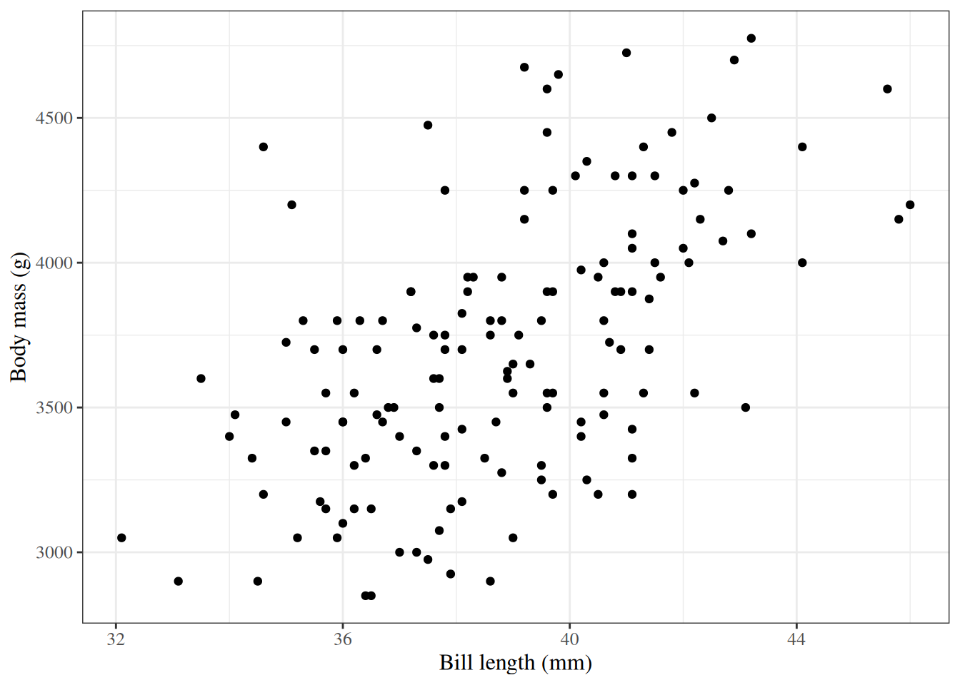
6.2 Example: Adelie penguins
Figure 1: Palmer penguins
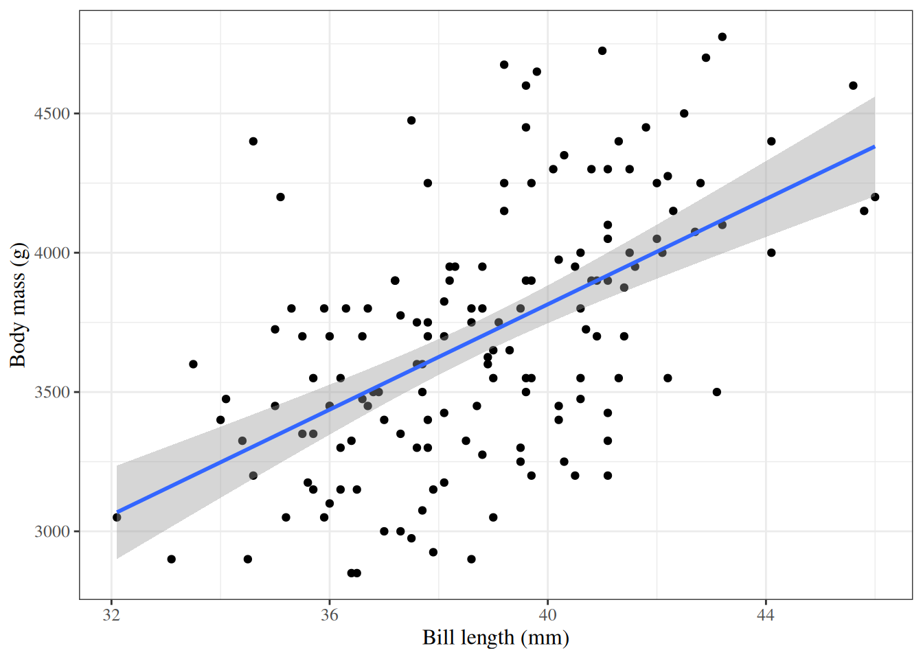
6.3 Linear regression
Show R code
ggpenguins2<-ggpenguins+stat_smooth( method ="lm", formula =y~x, geom ="smooth")ggpenguins2|>print()
Figure 2: Palmer penguins with linear regression fit
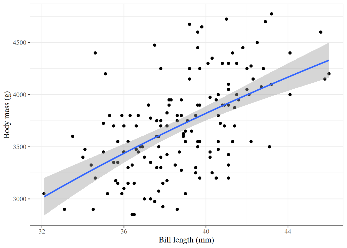
6.4 Curved regression lines
Show R code
ggpenguins2<-ggpenguins+stat_smooth( method ="lm", formula =y~log(x), geom ="smooth")+xlab("Bill length (mm)")+ylab("Body mass (g)")ggpenguins2
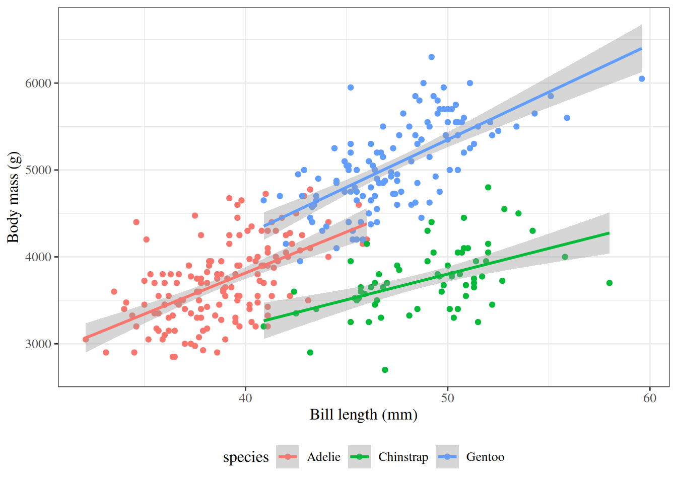
ggpenguins<-palmerpenguins::penguins|>ggplot(aes( x =bill_length_mm, y =body_mass_g, color =species))+geom_point()+stat_smooth( method ="lm", formula =y~x, geom ="smooth")+xlab("Bill length (mm)")+ylab("Body mass (g)")ggpenguins|>print()
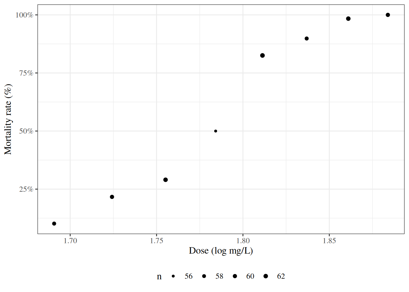
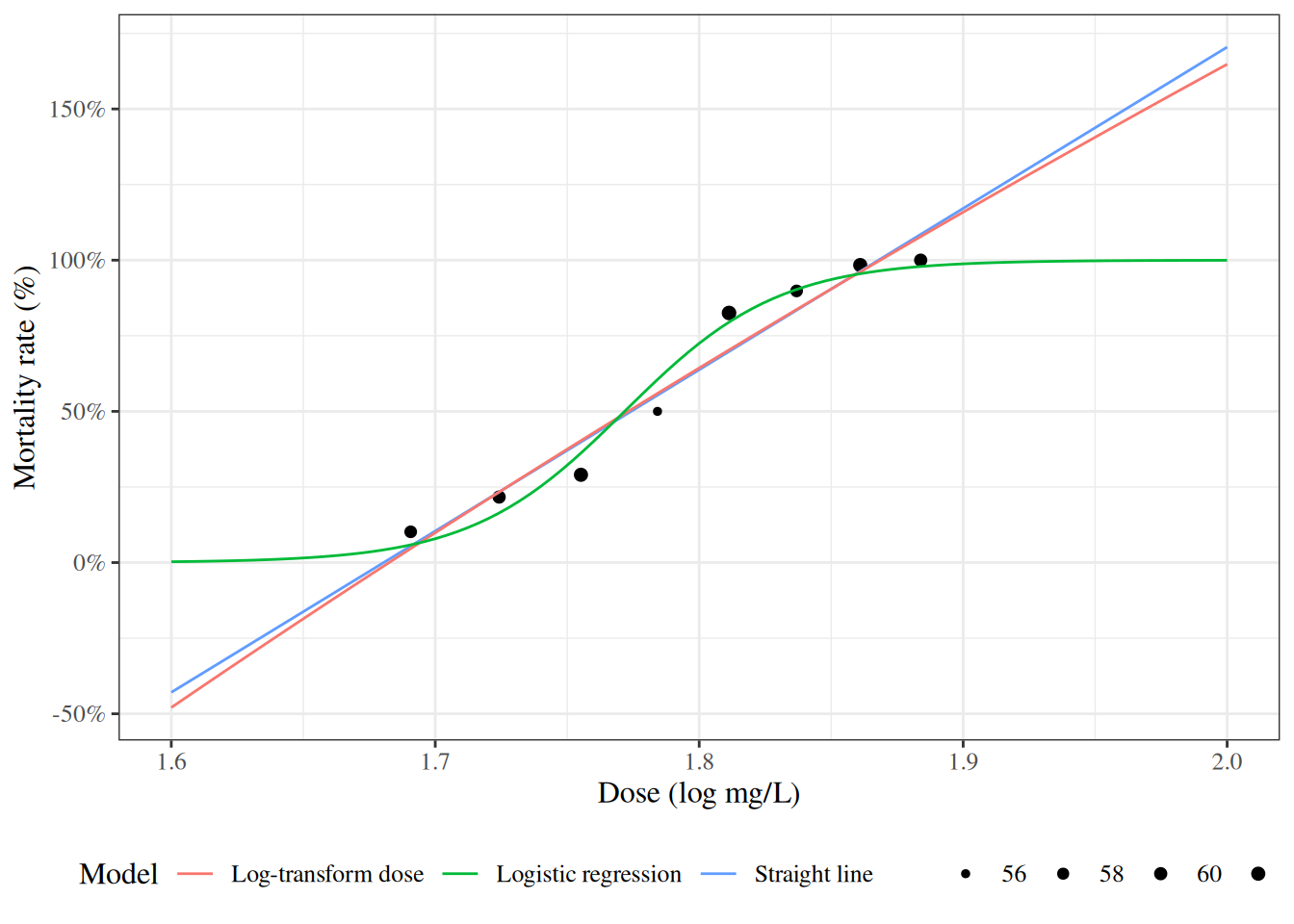
Figure 5: Mortality rates of adult flour beetles after five hours’ exposure to gaseous carbon disulphide (Bliss 1935). The dose column holds the base-10 logarithm of the dose in mg/L, and the models use it as is; the figures show the dose itself, in mg/L, on a log-spaced axis.
6.7 Why don’t we use linear regression?
Show R code
beetles_long<-beetles|>reframe( .by =everything(), outcome =c(rep(1, times =died),rep(0, times =survived)))lm1<-beetles_long|>lm( formula =outcome~dose, data =_)f_linear<-function(x)predict(lm1, newdata =data.frame(dose =log10(x)))plot2<-plot1+geom_function(fun =f_linear, aes(col ="Straight line"))+labs(colour ="Model", size ="")print(plot2)
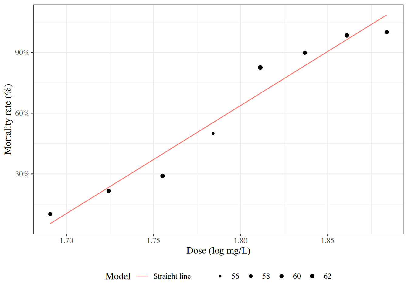
Figure 6: Mortality rates of adult flour beetles after five hours’ exposure to gaseous carbon disulphide (Bliss 1935)
6.8 Zoom out
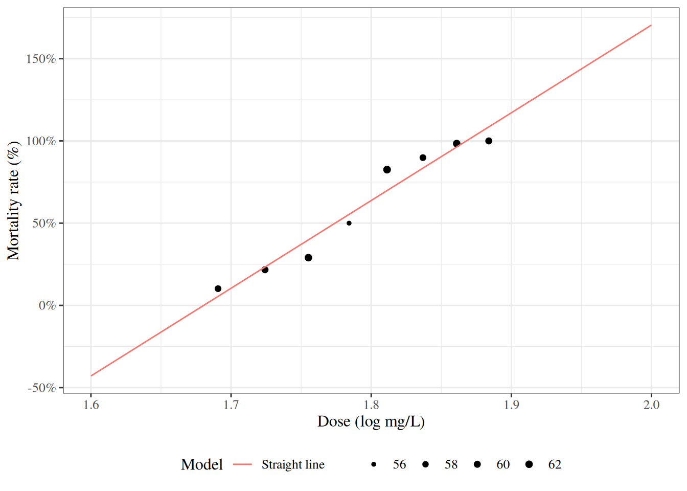
Figure 7: Mortality rates of adult flour beetles after five hours’ exposure to gaseous carbon disulphide (Bliss 1935)
Exercise 3 What are some of the names used for the variables in a regression model \(\mathbb{P}(Y|\mathord{\smash[b]{\underset{\raise.3ex\hbox{$\scriptstyle\sim$}}{X}}\vphantom{X}})\)?
Definition 2 (Outcome (response variable, regressand, predicted variable, explained variable, experimental variable, output variable, dependent variable, endogenous variable, target, label)) The outcome variable in a regression model is the variable whose distribution is being described; in other words, the variable on the left-hand side of the “|” (“pipe”) symbol.
It is also called the response variable, regressand, predicted variable, explained variable, experimental variable, output variable, dependent variable, endogenous variable, target, or label.
Definition 3 (Predictors (regressors, covariates, independent variables, explanatory variables, risk factors, exposure variables, input variables, exogenous variables, candidate variables, carriers, manipulated variables, features)) The predictor variables in a regression model are the conditioning variables defining subpopulations among which the outcome distribution might vary.
Predictors are also called regressors, covariates, independent variables, explanatory variables, risk factors, exposure variables, input variables, exogenous variables, candidate variables (Dunn and Smyth [9]), carriers (Dunn and Smyth [9]), manipulated variables, or features and are typically denoted \(\mathord{\smash[b]{\underset{\raise.3ex\hbox{$\scriptstyle\sim$}}{X}}\vphantom{X}}\). 2
Table 3: Common pairings of terms for variables \(\mathord{\smash[b]{\underset{\raise.3ex\hbox{$\scriptstyle\sim$}}{X}}\vphantom{X}}\) and \(Y\) in regression models \(P(Y|\mathord{\smash[b]{\underset{\raise.3ex\hbox{$\scriptstyle\sim$}}{X}}\vphantom{X}})\)3
Solution 2. Generalized linear models have three components:
The outcome distribution family: \(\operatorname{p}(Y|\mu(\mathord{\smash[b]{\underset{\raise.3ex\hbox{$\scriptstyle\sim$}}{x}}\vphantom{x}}))\)
The link function: \(g(\mu(\mathord{\smash[b]{\underset{\raise.3ex\hbox{$\scriptstyle\sim$}}{x}}\vphantom{x}})) = \eta(\mathord{\smash[b]{\underset{\raise.3ex\hbox{$\scriptstyle\sim$}}{x}}\vphantom{x}})\)
The linear component: \(\eta(\mathord{\smash[b]{\underset{\raise.3ex\hbox{$\scriptstyle\sim$}}{x}}\vphantom{x}}) = \mathord{\smash[b]{\underset{\raise.3ex\hbox{$\scriptstyle\sim$}}{x}}\vphantom{x}}\cdot \beta\)
The outcome distribution family (a.k.a. the random component of the model)
Definition 4 (Linear predictor (linear component)) Let \(\mathord{\smash[b]{\underset{\raise.3ex\hbox{$\scriptstyle\sim$}}{x}}\vphantom{x}}\stackrel{\text{def}}{=}{(1, x_1, \ldots, x_p)}^{\top}\) be a covariate vector, with a leading 1 for the intercept, and let \(\mathord{\smash[b]{\underset{\raise.3ex\hbox{$\scriptstyle\sim$}}{\beta}}\vphantom{\beta}}\stackrel{\text{def}}{=}{(\beta_0, \beta_1, \ldots, \beta_p)}^{\top}\) be a vector of regression coefficients. The linear predictor (or linear component) of a regression model is the function
Example 4 (Computing a linear predictor) Suppose a model has one covariate, dose \(x\), with coefficients \(\beta_0 = -60\) and \(\beta_1 = 34\). At dose \(x = 1.8\):
The model \(\eta(\mathord{\smash[b]{\underset{\raise.3ex\hbox{$\scriptstyle\sim$}}{x}}\vphantom{x}}) = \beta_0 + \beta_1 {\operatorname{log}\mathopen{}\left\{x\right\}\mathclose{}} + \beta_2 x^2\) also has a linear predictor, with covariates \(x_1 \stackrel{\text{def}}{=}{\operatorname{log}\mathopen{}\left\{x\right\}\mathclose{}}\) and \(x_2 \stackrel{\text{def}}{=}x^2\): it is a weighted sum of covariates with weights \(\beta_0, \beta_1, \beta_2\).
RemarkRemark 1 (Linear in the coefficients, not in the covariates)
Remark 1 (Linear in the coefficients, not in the covariates). The linear predictor must be linear in the coefficients\(\mathord{\smash[b]{\underset{\raise.3ex\hbox{$\scriptstyle\sim$}}{\beta}}\vphantom{\beta}}\); it need not be linear in the original covariates, because each \(x_j\) can itself be a transformation of the data, such as \({\operatorname{log}\mathopen{}\left\{\text{dose}\right\}\mathclose{}}\), \(\text{age}^2\), or a product of two covariates.
ExmExample 5 (A function that is not a linear predictor)
Example 5 (A function that is not a linear predictor) The function \(\eta(x) = \beta_0 + x^{\beta_1}\) is not a linear predictor, because \(\beta_1\) enters as an exponent rather than as a multiplier of a covariate. For example, at \(x = 2\), increasing \(\beta_1\) from 1 to 2 changes \(x^{\beta_1}\) from \(2\) to \(4\), an increase of 2, but increasing \(\beta_1\) from 2 to 3 changes \(x^{\beta_1}\) from \(4\) to \(8\), an increase of 4. A linear function of \(\beta_1\) would change by the same amount for each equal step in \(\beta_1\).
Definition 5 (Link function) Let \(\mu(\mathord{\smash[b]{\underset{\raise.3ex\hbox{$\scriptstyle\sim$}}{x}}\vphantom{x}}) \stackrel{\text{def}}{=}{\mathbb{E}\mathopen{}\left[Y|\mathord{\smash[b]{\underset{\raise.3ex\hbox{$\scriptstyle\sim$}}{X}}\vphantom{X}}=\mathord{\smash[b]{\underset{\raise.3ex\hbox{$\scriptstyle\sim$}}{x}}\vphantom{x}}\right]\mathclose{}}\) be the conditional mean of the outcome. A link function is a monotone, differentiable function \(g(\cdot)\) that relates the mean to the linear predictor (Definition 4):
Definition 6 (Inverse link) When \(g\) is strictly monotone on the range of possible means, it has an inverse, the inverse link\(g^{-1}(\cdot)\), which maps the linear predictor back to the mean:
Example 6 (Logit and log links) Take \(\eta = 1.2\) from Example 4. With the logit link \(g(\mu) = \operatorname{logit}(\mu) = {\operatorname{log}\mathopen{}\left\{\frac{\mu}{1-\mu}\right\}\mathclose{}}\), the inverse link is \(g^{-1}(\eta) = \operatorname{expit}(\eta) = \frac{1}{1 + e^{-\eta}}\), so:
With the log link \(g(\mu) = {\operatorname{log}\mathopen{}\left\{\mu\right\}\mathclose{}}\) instead, the inverse link is \(g^{-1}(\eta) = {\operatorname{exp}\mathopen{}\left\{\eta\right\}\mathclose{}}\), so the same linear predictor gives \(\mu = e^{1.2} \approx 3.320\).
ExmExample 7 (A function that is not a link function)
Example 7 (A function that is not a link function) For a Gaussian outcome, whose mean can be any real number, \(g(\mu) = \mu^2\) is not a valid link function, because it is not monotone on \((-\infty, \infty)\). Both \(\mu = -1\) and \(\mu = 1\) give \(g(\mu) = 1\), so a linear predictor \(\eta(\mathord{\smash[b]{\underset{\raise.3ex\hbox{$\scriptstyle\sim$}}{x}}\vphantom{x}}) = 1\) does not determine the mean, and \(g\) has no inverse link.
DefDefinition 7 (Outcome distribution (random component))
Definition 7 (Outcome distribution (random component)) In a regression model (Definition 1) for an outcome \(Y\) given covariates \(\mathord{\smash[b]{\underset{\raise.3ex\hbox{$\scriptstyle\sim$}}{X}}\vphantom{X}}= \mathord{\smash[b]{\underset{\raise.3ex\hbox{$\scriptstyle\sim$}}{x}}\vphantom{x}}\), the outcome distribution family (the random component) is the specified distribution family that \(Y\) follows given \(\mathord{\smash[b]{\underset{\raise.3ex\hbox{$\scriptstyle\sim$}}{X}}\vphantom{X}}= \mathord{\smash[b]{\underset{\raise.3ex\hbox{$\scriptstyle\sim$}}{x}}\vphantom{x}}\), such as Gaussian, Bernoulli, or Poisson, with conditional mean \(\mu(\mathord{\smash[b]{\underset{\raise.3ex\hbox{$\scriptstyle\sim$}}{x}}\vphantom{x}}) \stackrel{\text{def}}{=}{\mathbb{E}\mathopen{}\left[Y|\mathord{\smash[b]{\underset{\raise.3ex\hbox{$\scriptstyle\sim$}}{X}}\vphantom{X}}=\mathord{\smash[b]{\underset{\raise.3ex\hbox{$\scriptstyle\sim$}}{x}}\vphantom{x}}\right]\mathclose{}}\), where observations are independent given their covariates [9, Ch. 5], [10, Ch. 3].
Definition 8 (Generalized linear model) A generalized linear model (GLM) is a regression model (Definition 1) for an outcome \(Y\) given covariates \(\mathord{\smash[b]{\underset{\raise.3ex\hbox{$\scriptstyle\sim$}}{X}}\vphantom{X}}= \mathord{\smash[b]{\underset{\raise.3ex\hbox{$\scriptstyle\sim$}}{x}}\vphantom{x}}\) with three components [9, Ch. 5], [10, Ch. 3]:
an outcome distribution family (the random component): given \(\mathord{\smash[b]{\underset{\raise.3ex\hbox{$\scriptstyle\sim$}}{X}}\vphantom{X}}= \mathord{\smash[b]{\underset{\raise.3ex\hbox{$\scriptstyle\sim$}}{x}}\vphantom{x}}\), \(Y\) follows a specified distribution family, such as Gaussian, Bernoulli, or Poisson, with conditional mean \(\mu(\mathord{\smash[b]{\underset{\raise.3ex\hbox{$\scriptstyle\sim$}}{x}}\vphantom{x}}) \stackrel{\text{def}}{=}{\mathbb{E}\mathopen{}\left[Y|\mathord{\smash[b]{\underset{\raise.3ex\hbox{$\scriptstyle\sim$}}{X}}\vphantom{X}}=\mathord{\smash[b]{\underset{\raise.3ex\hbox{$\scriptstyle\sim$}}{x}}\vphantom{x}}\right]\mathclose{}}\), and observations are independent given their covariates (Definition 7);
a linear predictor \(\eta(\mathord{\smash[b]{\underset{\raise.3ex\hbox{$\scriptstyle\sim$}}{x}}\vphantom{x}}) = {\mathord{\smash[b]{\underset{\raise.3ex\hbox{$\scriptstyle\sim$}}{x}}\vphantom{x}}}^{\top}\mathord{\smash[b]{\underset{\raise.3ex\hbox{$\scriptstyle\sim$}}{\beta}}\vphantom{\beta}}\) (Definition 4);
a link function \(g\) connecting the two, \(g\mathopen{}\left(\mu(\mathord{\smash[b]{\underset{\raise.3ex\hbox{$\scriptstyle\sim$}}{x}}\vphantom{x}})\right)\mathclose{} = \eta(\mathord{\smash[b]{\underset{\raise.3ex\hbox{$\scriptstyle\sim$}}{x}}\vphantom{x}})\) (Definition 5).
A GLM specifies model structure only: its coefficients \(\mathord{\smash[b]{\underset{\raise.3ex\hbox{$\scriptstyle\sim$}}{\beta}}\vphantom{\beta}}\) can be estimated by maximum likelihood, by Bayesian methods, or by other inference methods.
ExmExample 8 (Logistic and linear regression as GLMs)
Example 8 (Logistic and linear regression as GLMs) Let \(Y \in \{0, 1\}\) indicate death of a beetle exposed to dose \(x\). The model with
outcome distribution \(Y|X=x \sim \operatorname{Bernoulli}\mathopen{}\left(\mu(x)\right)\mathclose{}\),
linear predictor \(\eta(x) = \beta_0 + \beta_1 x\),
logit link \(\operatorname{logit}\mathopen{}\left(\mu(x)\right)\mathclose{} = \eta(x)\)
is a GLM: logistic regression. With \(\beta_0 = -60\) and \(\beta_1 = 34\), Example 4 and Example 6 give \(\eta(1.8) = 1.2\) and \(\mathbb{P}(Y=1|X=1.8) = \mu(1.8) \approx 0.7685\).
The Gaussian linear regression model \(Y|X=x \sim {\operatorname{N}\mathopen{}\left(\beta_0 + \beta_1 x, \sigma^2\right)\mathclose{}}\) is also a GLM, with a Gaussian outcome distribution and the identity link \(g(\mu) = \mu\), so that \(\mu(x) = \eta(x)\).
Definition 9 (Interaction) Consider a regression model whose linear predictor \(\eta(\mathord{\smash[b]{\underset{\raise.3ex\hbox{$\scriptstyle\sim$}}{x}}\vphantom{x}})\) includes two covariates \(x_j\) and \(x_k\). The model includes an interaction between \(x_j\) and \(x_k\) when the difference in \(\eta(\mathord{\smash[b]{\underset{\raise.3ex\hbox{$\scriptstyle\sim$}}{x}}\vphantom{x}})\) per unit difference in \(x_j\), holding the other covariates fixed, depends on the value of \(x_k\)[10, Ch. 6].
Definition 9 describes only how the linear predictor varies across subpopulations, so it makes no causal claim. Interaction is also scale-dependent: Definition 9 is stated on the scale of the linear predictor \(\eta(\mathord{\smash[b]{\underset{\raise.3ex\hbox{$\scriptstyle\sim$}}{x}}\vphantom{x}})\), which can differ from the scale of the mean \(\mu(\mathord{\smash[b]{\underset{\raise.3ex\hbox{$\scriptstyle\sim$}}{x}}\vphantom{x}})\).
Definition 10 (Interaction term) An interaction term is a term in the linear predictor formed by multiplying two (or more) covariates together, such as \(\beta_{jk} x_j x_k\); its coefficient \(\beta_{jk}\) is called an interaction coefficient. A linear predictor with two covariates and their interaction term has the form:
ExmExample 9 (A linear predictor with an interaction term)
Example 9 (A linear predictor with an interaction term) Suppose a model has a numeric covariate \(x\), a binary covariate \(z \in \{0, 1\}\), and linear predictor
\[\eta(x, z) = 1 + 2x + 3z + 4xz.\]
The difference in \(\eta\) per unit difference in \(x\), holding \(z\) fixed, is:
When \(z = 0\): the difference is \(2 + 4 \cdot 0 = 2\).
When \(z = 1\): the difference is \(2 + 4 \cdot 1 = 6\).
The difference per unit of \(x\) depends on \(z\), so this model includes an interaction between \(x\) and \(z\), and \(4xz\) is its interaction term, with interaction coefficient \(4\).
ExmExample 10 (A linear predictor without an interaction term (counterexample))
Example 10 (A linear predictor without an interaction term (counterexample)) Now drop the interaction term, so that \(\eta(x, z) = 1 + 2x + 3z\). Then:
The difference per unit of \(x\) is \(2\) at both \(z = 0\) and \(z = 1\), so this model has no interaction between \(x\) and \(z\): the lines for \(z = 0\) and \(z = 1\) are parallel on the scale of \(\eta\).
8 Why link functions?
So far, we have seen models for Gaussian distributions that vary across subpopulations, and distributions for single populations. A GLM combines the two: it describes how a non-Gaussian distribution varies across subpopulations. The link function is the piece that makes this work.
Exercise 5 Suppose the outcome is a count or a binary variable. Why not model the mean \(\mu(\mathord{\smash[b]{\underset{\raise.3ex\hbox{$\scriptstyle\sim$}}{x}}\vphantom{x}})\) as a linear function of the covariates, as in a Gaussian model?
Solution 3. A straight line for \(\mu(\mathord{\smash[b]{\underset{\raise.3ex\hbox{$\scriptstyle\sim$}}{x}}\vphantom{x}})\) can leave the range of the outcome: it can predict a negative count, or a probability below 0 or above 1. We could try to repair this by transforming each covariate separately and adding interaction terms (Definition 9) until the fitted curve stays in range, but that is hard to get right.
The link function offers a simpler route. We add all the covariate terms together first, to get the linear predictor\(\eta(\mathord{\smash[b]{\underset{\raise.3ex\hbox{$\scriptstyle\sim$}}{x}}\vphantom{x}})\), and then transform once, with the inverse link \(g^{-1}\). The link \(g\) relates the mean to the linear predictor: \(g\mathopen{}\left(\mu(\mathord{\smash[b]{\underset{\raise.3ex\hbox{$\scriptstyle\sim$}}{x}}\vphantom{x}})\right)\mathclose{} = \eta(\mathord{\smash[b]{\underset{\raise.3ex\hbox{$\scriptstyle\sim$}}{x}}\vphantom{x}})\). Applying \(g^{-1}\) to both sides gives:
Choosing the inverse link guarantees the model structure we want:
with the log link, \(\mu(\mathord{\smash[b]{\underset{\raise.3ex\hbox{$\scriptstyle\sim$}}{x}}\vphantom{x}}) = {\operatorname{exp}\mathopen{}\left\{\eta(\mathord{\smash[b]{\underset{\raise.3ex\hbox{$\scriptstyle\sim$}}{x}}\vphantom{x}})\right\}\mathclose{}} > 0\), so a mean count is never negative;
with the logit link, \(\mu(\mathord{\smash[b]{\underset{\raise.3ex\hbox{$\scriptstyle\sim$}}{x}}\vphantom{x}}) = \operatorname{expit}(\eta(\mathord{\smash[b]{\underset{\raise.3ex\hbox{$\scriptstyle\sim$}}{x}}\vphantom{x}}))\) lies in \((0, 1)\), so a probability is never below 0 or above 1.
Remark 2 (Slopes under a non-identity link). With a non-identity link, interpreting a slope gets harder. A coefficient \(\beta_j\) is the change in \(g(\mu)\) per unit change in \(x_j\), not the change in \(\mu\). Even without any interaction terms (Definition 9), the change in \(\mu\) per unit change in \(x_j\) depends on the values of the other covariates, because \(g^{-1}\) is not linear.
ExmExample 11 (A logistic model with no interaction)
Example 11 (A logistic model with no interaction) Suppose the mean \(\mu\) of a binary outcome, which is its probability, satisfies \(\operatorname{logit}(\mu) = -2 + 1 \cdot x + 1.5 \cdot z\), with \(z \in \{0, 1\}\). The coefficient of \(x\) is the same at both values of \(z\), so the odds ratio for a one-unit increase in \(x\) is \(e^1\) at both values of \(z\). The code below computes the change in probability for the same increase in \(x\), from \(x = 0\) to \(x = 1\).
For \(z = 0\), the probability rises by 0.15; for \(z = 1\), it rises by 0.245. The odds ratio is the same in both subgroups, but the difference in probabilities is not.
9 Canonical links
The link functions listed in the structure of a GLM are not all on the same footing. For each outcome distribution, the form of its density singles out one link. To say which, we need the density’s natural parameter.
Definition 11 (Exponential dispersion family) A distribution belongs to the exponential dispersion family if its density (or probability mass function) can be written as
Definition 12 (Natural parameter) In an exponential dispersion family (Definition 11), the parameter \(\theta\) is the natural parameter[9, Ch. 5], [10, Ch. 3].
Definition 13 (Dispersion parameter) In an exponential dispersion family (Definition 11), the parameter \(\phi > 0\) is the dispersion parameter[9, Ch. 5], [10, Ch. 3].
ExmExample 12 (Poisson and Bernoulli distributions in exponential dispersion form)
Example 12 (Poisson and Bernoulli distributions in exponential dispersion form) For a Poisson outcome with mean \(\mu\),
so \(\theta \stackrel{\text{def}}{=}{\operatorname{log}\mathopen{}\left\{\mu\right\}\mathclose{}}\), \(b(\theta) \stackrel{\text{def}}{=}e^\theta\), and \(\phi \stackrel{\text{def}}{=}1\). For a Bernoulli outcome with success probability \(\pi\),
so \(\theta \stackrel{\text{def}}{=}\operatorname{logit}(\pi)\), \(b(\theta) \stackrel{\text{def}}{=}{\operatorname{log}\mathopen{}\left\{1 + e^\theta\right\}\mathclose{}}\), and \(\phi \stackrel{\text{def}}{=}1\).
The code below checks both forms against R’s built-in densities, at \(\mu = 3\), \(y = 2\) and at \(\pi = 0.25\), \(y = 1\).
For the Poisson distribution with \(\mu = 3\), the natural parameter is \(\theta = \log(3) =\) 1.0986, and the exponential-family form gives \(f(2) =\) 0.224, which matches dpois(2, 3): TRUE.
For the Bernoulli distribution with \(\pi = 0.25\), the natural parameter is \(\theta = \operatorname{logit}(0.25) =\) -1.0986, and the exponential-family form gives \(f(1) =\) 0.25, which matches dbinom(1, 1, 0.25): TRUE.
ExmExample 13 (The Gaussian distribution in exponential dispersion form)
Example 13 (The Gaussian distribution in exponential dispersion form) For a Gaussian outcome \(Y \sim {\operatorname{N}\mathopen{}\left(\mu, \sigma^2\right)\mathclose{}}\):
\[
\begin{aligned}
f(y; \mu, \sigma^2)
&= \frac{1}{\sqrt{2\pi\sigma^2}} {\operatorname{exp}\mathopen{}\left\{-\frac{(y - \mu)^2}{2\sigma^2}\right\}\mathclose{}}
&& \text{(Gaussian density)}
\\ &= {\operatorname{exp}\mathopen{}\left\{-\frac{(y - \mu)^2}{2\sigma^2} - \frac{1}{2}{\operatorname{log}\mathopen{}\left\{2\pi\sigma^2\right\}\mathclose{}}\right\}\mathclose{}}
&& \text{(write the constant as the exponential of its log)}
\\ &= {\operatorname{exp}\mathopen{}\left\{-\frac{y^2 - 2y\mu + \mu^2}{2\sigma^2} - \frac{1}{2}{\operatorname{log}\mathopen{}\left\{2\pi\sigma^2\right\}\mathclose{}}\right\}\mathclose{}}
&& \text{(expand the square)}
\\ &= {\operatorname{exp}\mathopen{}\left\{\frac{y\mu - \mu^2/2}{\sigma^2} - \frac{y^2}{2\sigma^2} - \frac{1}{2}{\operatorname{log}\mathopen{}\left\{2\pi\sigma^2\right\}\mathclose{}}\right\}\mathclose{}}
&& \text{(distribute the division over the sum, and simplify each term)}
\end{aligned}
\]
Matching this last line to Definition 11 gives \(\theta \stackrel{\text{def}}{=}\mu\), \(b(\theta) \stackrel{\text{def}}{=}\theta^2/2\), \(\phi \stackrel{\text{def}}{=}\sigma^2\), and \(c(y, \phi) \stackrel{\text{def}}{=}-\frac{y^2}{2\phi} - \frac{1}{2}{\operatorname{log}\mathopen{}\left\{2\pi\phi\right\}\mathclose{}}\).
For instance, take \(\mu = 2\), \(\sigma^2 = 4\), and \(y = 3\). The first term of the exponent is
and the second term is \(c(3, 4) = -\frac{9}{8} - \frac{1}{2}{\operatorname{log}\mathopen{}\left\{8\pi\right\}\mathclose{}}\), so the exponent is \(-\frac{1}{8} - \frac{1}{2}{\operatorname{log}\mathopen{}\left\{8\pi\right\}\mathclose{}}\). The Gaussian density’s own exponent is also \(-\frac{(3 - 2)^2}{8} - \frac{1}{2}{\operatorname{log}\mathopen{}\left\{8\pi\right\}\mathclose{}} = -\frac{1}{8} - \frac{1}{2}{\operatorname{log}\mathopen{}\left\{8\pi\right\}\mathclose{}}\), and both forms give \(f(3) \approx 0.1760\).
LemTheorem 1 (Mean and variance in an exponential dispersion family)
Theorem 1 (Mean and variance in an exponential dispersion family) Let \(Y\) have the density \(f(y; \theta, \phi)\) of Definition 11, and suppose that the support of \(Y\) does not depend on \(\theta\) and that \(b\) is twice differentiable. Then
Proof. We write the proof with integrals; for a probability mass function, replace each integral with a sum. Because the support does not depend on \(\theta\), we can differentiate under the integral sign.
The derivative of the density with respect to \(\theta\) is
\[
\begin{aligned}
\frac{\partial}{\partial \theta} f(y; \theta, \phi)
&= f(y; \theta, \phi)
\frac{\partial}{\partial \theta}\mathopen{}\left[\frac{y\theta - b(\theta)}{\phi} + c(y, \phi)\right]\mathclose{}
&& \text{(chain rule for the exponential)}
\\ &= f(y; \theta, \phi) \frac{y - b'(\theta)}{\phi}
&& \text{(differentiate term by term)}
\end{aligned}
\]
Every density integrates to 1, for every value of \(\theta\), so differentiating that identity once gives the mean:
\[
\begin{aligned}
0 &= \frac{\partial}{\partial \theta} \int f(y; \theta, \phi)\, dy
&& \text{(derivative of the constant 1)}
\\ &= \int \frac{\partial}{\partial \theta} f(y; \theta, \phi)\, dy
&& \text{(differentiate under the integral)}
\\ &= \int \frac{y - b'(\theta)}{\phi} f(y; \theta, \phi)\, dy
&& \text{(derivative of the density)}
\\ &= \frac{{\mathbb{E}\mathopen{}\left[Y\right]\mathclose{}} - b'(\theta)}{\phi}
&& \text{(definition of expectation, and } \textstyle\int f = 1\text{)}
\end{aligned}
\]
Multiplying both sides by \(\phi > 0\) gives \({\mathbb{E}\mathopen{}\left[Y\right]\mathclose{}} = b'(\theta)\).
Differentiating the same identity a second time gives the variance:
\[
\begin{aligned}
0 &= \frac{\partial}{\partial \theta} \int \frac{y - b'(\theta)}{\phi} f(y; \theta, \phi)\, dy
&& \text{(derivative of the constant 0)}
\\ &= \int \mathopen{}\left[-\frac{b''(\theta)}{\phi} f(y; \theta, \phi)
+ \frac{y - b'(\theta)}{\phi} \frac{\partial}{\partial \theta} f(y; \theta, \phi)\right]\mathclose{} dy
&& \text{(product rule)}
\\ &= \int \mathopen{}\left[-\frac{b''(\theta)}{\phi}
+ \frac{\mathopen{}\left(y - b'(\theta)\right)\mathclose{}^2}{\phi^2}\right]\mathclose{} f(y; \theta, \phi)\, dy
&& \text{(derivative of the density)}
\\ &= -\frac{b''(\theta)}{\phi} + \frac{{\mathbb{E}\mathopen{}\left[\mathopen{}\left(Y - b'(\theta)\right)\mathclose{}^2\right]\mathclose{}}}{\phi^2}
&& \text{(definition of expectation, and } \textstyle\int f = 1\text{)}
\\ &= -\frac{b''(\theta)}{\phi} + \frac{{\operatorname{Var}\mathopen{}\left(Y\right)\mathclose{}}}{\phi^2}
&& \text{(} b'(\theta) = {\mathbb{E}\mathopen{}\left[Y\right]\mathclose{}}\text{, so this is the variance)}
\end{aligned}
\]
Multiplying both sides by \(\phi^2\) and rearranging gives \({\operatorname{Var}\mathopen{}\left(Y\right)\mathclose{}} = \phi\, b''(\theta)\).
ExmExample 14 (Means and variances from \(b(\theta)\))
Example 14 (Means and variances from \(b(\theta)\)) We apply Theorem 1 to the distributions in Example 12 and Example 13.
Gaussian, with \(b(\theta) = \theta^2/2\) and \(\phi = \sigma^2\): \(b'(\theta) = \theta = \mu\) and \(b''(\theta) = 1\), so \({\mathbb{E}\mathopen{}\left[Y\right]\mathclose{}} = \mu\) and \({\operatorname{Var}\mathopen{}\left(Y\right)\mathclose{}} = \sigma^2 \cdot 1 = \sigma^2\). With \(\mu = 2\) and \(\sigma^2 = 4\), \({\mathbb{E}\mathopen{}\left[Y\right]\mathclose{}} = 2\) and \({\operatorname{Var}\mathopen{}\left(Y\right)\mathclose{}} = 4\).
Poisson, with \(b(\theta) = e^\theta\) and \(\phi = 1\): \(b'(\theta) = b''(\theta) = e^\theta\). With \(\mu = 3\), so that \(\theta = {\operatorname{log}\mathopen{}\left\{3\right\}\mathclose{}}\), \({\mathbb{E}\mathopen{}\left[Y\right]\mathclose{}} = e^{{\operatorname{log}\mathopen{}\left\{3\right\}\mathclose{}}} = 3\) and \({\operatorname{Var}\mathopen{}\left(Y\right)\mathclose{}} = 1 \cdot e^{{\operatorname{log}\mathopen{}\left\{3\right\}\mathclose{}}} = 3\).
For the Bernoulli distribution, \(b(\theta) = {\operatorname{log}\mathopen{}\left\{1 + e^\theta\right\}\mathclose{}}\) and \(\phi = 1\), so:
With \(\pi = 0.25\), so that \(\theta = \operatorname{logit}(0.25)\) and \(\operatorname{expit}(\theta) = 0.25\), \({\mathbb{E}\mathopen{}\left[Y\right]\mathclose{}} = 0.25\) and \({\operatorname{Var}\mathopen{}\left(Y\right)\mathclose{}} = 0.25 \cdot 0.75 = 0.1875\).
Each result matches the familiar mean and variance of that distribution.
Definition 14 (Variance function) In an exponential dispersion family (Definition 11), \(V(\mu) \stackrel{\text{def}}{=}b''(\theta)\), written as a function of \(\mu \stackrel{\text{def}}{=}b'(\theta)\), is the variance function.
ExmExample 15 (Variance functions of three families)
Example 15 (Variance functions of three families) Rewriting each \(b''(\theta)\) from Example 14 as a function of the mean \(\mu = b'(\theta)\) gives each family’s variance function:
The Gaussian variance function is constant, so the variance does not depend on the mean. The Poisson variance function grows with the mean. The Bernoulli variance function is largest at \(\mu = 0.5\) and shrinks toward 0 as \(\mu\) approaches 0 or 1.
RemarkRemark 3 (The variance function and the variance)
Remark 3 (The variance function and the variance). By Theorem 1 and Definition 14, \({\operatorname{Var}\mathopen{}\left(Y\right)\mathclose{}} = \phi\, V(\mu)\).
Definition 15 (Canonical link) In an exponential dispersion family (Definition 11), the canonical link is the link function \(g(\cdot)\) (Definition 5) that sets the linear predictor equal to the natural parameter: \(g(\mu) \stackrel{\text{def}}{=}\theta\)[9, Ch. 5], [10, Ch. 3].
Theorem 2 (The canonical link inverts \(b'\)) In an exponential dispersion family (Definition 11) that satisfies the conditions of Theorem 1, with \(b''(\theta) > 0\) for every \(\theta\), the canonical link is the inverse of \(b'\):
Proof. Because \(b''(\theta) > 0\) for every \(\theta\), \(b'\) is strictly increasing, so it has an inverse \({\mathopen{}\left(b'\right)\mathclose{}}^{-1}\) on its range. By Theorem 1:
\[
\begin{aligned}
\mu &= b'(\theta)
&& \text{(mean of an exponential dispersion family)}
\\ {\mathopen{}\left(b'\right)\mathclose{}}^{-1}(\mu) &= \theta
&& \text{(apply } {\mathopen{}\left(b'\right)\mathclose{}}^{-1} \text{ to both sides)}
\\ &= g(\mu)
&& \text{(definition of the canonical link)}
\end{aligned}
\]
The condition \(b''(\theta) > 0\) holds for any distribution whose variance \(\phi\, b''(\theta)\) is positive, that is, any distribution that is not concentrated at a single value.
Example 16 (Canonical links of three families) We apply Theorem 2, using \(b'(\theta)\) from Example 14.
Gaussian: \(b'(\theta) = \theta\), so \({\mathopen{}\left(b'\right)\mathclose{}}^{-1}(\mu) = \mu\), and the canonical link is the identity link \(g(\mu) = \mu\).
Poisson: \(\mu = b'(\theta) = e^\theta\), so \(\theta = {\operatorname{log}\mathopen{}\left\{\mu\right\}\mathclose{}}\), and the canonical link is the log link \(g(\mu) = {\operatorname{log}\mathopen{}\left\{\mu\right\}\mathclose{}}\). At \(\mu = 3\), \(g(3) = {\operatorname{log}\mathopen{}\left\{3\right\}\mathclose{}} \approx 1.0986\).
For the Bernoulli distribution, we solve \(\mu = b'(\theta) = \operatorname{expit}(\theta)\) for \(\theta\):
So the canonical link is the logit link. At \(\mu = 0.25\), \(g(0.25) = {\operatorname{log}\mathopen{}\left\{0.25 / 0.75\right\}\mathclose{}} = {\operatorname{log}\mathopen{}\left\{1/3\right\}\mathclose{}} \approx -1.0986\).
Example 17 (A link that is not canonical) The probit link \(g(\mu) = \Phi^{-1}(\mu)\), where \(\Phi\) is the standard Gaussian cumulative distribution function, is a valid link function for a Bernoulli outcome, because it is strictly increasing on \((0, 1)\). It is not the canonical link: at \(\mu = 0.25\), \(\Phi^{-1}(0.25) \approx -0.6745\), whereas the natural parameter is \(\theta = \operatorname{logit}(0.25) \approx -1.0986\) (Example 16).
9.1 The score function under a canonical link
LemTheorem 3 (Score function of a GLM with a canonical link)
Theorem 3 (Score function of a GLM with a canonical link) Consider a GLM (Definition 8) for independent outcomes \(Y_1, \ldots, Y_n\) with covariate vectors \(\mathord{\smash[b]{\underset{\raise.3ex\hbox{$\scriptstyle\sim$}}{x}}\vphantom{x}}_1, \ldots, \mathord{\smash[b]{\underset{\raise.3ex\hbox{$\scriptstyle\sim$}}{x}}\vphantom{x}}_n\), whose outcome distribution is an exponential dispersion family (Definition 11) satisfying the conditions of Theorem 1, with natural parameters \(\theta_i\) and a common dispersion parameter \(\phi\), and whose link is the canonical link (Definition 15). Write \(\mu_i \stackrel{\text{def}}{=}{\mathbb{E}\mathopen{}\left[Y_i | \mathord{\smash[b]{\underset{\raise.3ex\hbox{$\scriptstyle\sim$}}{X}}\vphantom{X}}_i = \mathord{\smash[b]{\underset{\raise.3ex\hbox{$\scriptstyle\sim$}}{x}}\vphantom{x}}_i\right]\mathclose{}}\). Then the score function for \(\mathord{\smash[b]{\underset{\raise.3ex\hbox{$\scriptstyle\sim$}}{\beta}}\vphantom{\beta}}\) is
Proof. With the canonical link, the natural parameter of observation \(i\) is its linear predictor:
\[
\begin{aligned}
\theta_i &= g(\mu_i)
&& \text{(definition of the canonical link)}
\\ &= \eta(\mathord{\smash[b]{\underset{\raise.3ex\hbox{$\scriptstyle\sim$}}{x}}\vphantom{x}}_i)
&& \text{(definition of the link function)}
\\ &= {\mathord{\smash[b]{\underset{\raise.3ex\hbox{$\scriptstyle\sim$}}{x}}\vphantom{x}}_i}^{\top}\mathord{\smash[b]{\underset{\raise.3ex\hbox{$\scriptstyle\sim$}}{\beta}}\vphantom{\beta}}
&& \text{(definition of the linear predictor)}
\end{aligned}
\]
The log-likelihood contribution of observation \(i\) is
and its derivative with respect to \(\theta_i\) is
\[
\begin{aligned}
\frac{\partial}{\partial \theta_i} \ell_i
&= \frac{y_i - b'(\theta_i)}{\phi}
&& \text{(differentiate term by term)}
\\ &= \frac{y_i - \mu_i}{\phi}
&& \text{(the mean is } b'(\theta_i)\text{)}
\end{aligned}
\]
The derivative of \(\theta_i = {\mathord{\smash[b]{\underset{\raise.3ex\hbox{$\scriptstyle\sim$}}{x}}\vphantom{x}}_i}^{\top}\mathord{\smash[b]{\underset{\raise.3ex\hbox{$\scriptstyle\sim$}}{\beta}}\vphantom{\beta}}\) with respect to \(\mathord{\smash[b]{\underset{\raise.3ex\hbox{$\scriptstyle\sim$}}{\beta}}\vphantom{\beta}}\) is the vector \(\underbrace{\mathord{\smash[b]{\underset{\raise.3ex\hbox{$\scriptstyle\sim$}}{x}}\vphantom{x}}_i}_{(p+1) \times 1}\). So, by the chain rule:
The outcomes are independent, so the log-likelihood is the sum \(\ell(\mathord{\smash[b]{\underset{\raise.3ex\hbox{$\scriptstyle\sim$}}{\beta}}\vphantom{\beta}}) = \sum_{i=1}^n\ell_i(\mathord{\smash[b]{\underset{\raise.3ex\hbox{$\scriptstyle\sim$}}{\beta}}\vphantom{\beta}})\), and:
\[
\begin{aligned}
\mathord{\smash[b]{\underset{\raise.3ex\hbox{$\scriptstyle\sim$}}{\ell'}}\vphantom{\ell'}}(\mathord{\smash[b]{\underset{\raise.3ex\hbox{$\scriptstyle\sim$}}{\beta}}\vphantom{\beta}})
&= \sum_{i=1}^n\frac{\partial}{\partial \mathord{\smash[b]{\underset{\raise.3ex\hbox{$\scriptstyle\sim$}}{\beta}}\vphantom{\beta}}} \ell_i
&& \text{(derivative of a sum)}
\\ &= \sum_{i=1}^n\mathord{\smash[b]{\underset{\raise.3ex\hbox{$\scriptstyle\sim$}}{x}}\vphantom{x}}_i \frac{y_i - \mu_i}{\phi}
&& \text{(substitute each term)}
\\ &= \frac{1}{\phi} \sum_{i=1}^n\mathord{\smash[b]{\underset{\raise.3ex\hbox{$\scriptstyle\sim$}}{x}}\vphantom{x}}_i (y_i - \mu_i)
&& \text{(factor out } 1/\phi\text{)}
\end{aligned}
\]
Example 18 (Score of a logistic model) Logistic regression uses the canonical link for a Bernoulli outcome (Example 16), with \(\phi = 1\), so Equation 1 applies. Take \(n = 3\) observations with \(\mathord{\smash[b]{\underset{\raise.3ex\hbox{$\scriptstyle\sim$}}{x}}\vphantom{x}}_i = {(1, x_i)}^{\top}\), \(x = (0, 1, 2)\) and \(y = (0, 1, 1)\), and evaluate the score at \(\mathord{\smash[b]{\underset{\raise.3ex\hbox{$\scriptstyle\sim$}}{\beta}}\vphantom{\beta}}= {(0, 1)}^{\top}\). The fitted means are \(\mu_i = \operatorname{expit}(\beta_0 + \beta_1 x_i) = \operatorname{expit}(x_i)\):
ExmExample 19 (Score of a Poisson model with the identity link (counterexample))
Example 19 (Score of a Poisson model with the identity link (counterexample)) With a non-canonical link, Equation 1 need not hold. Take a Poisson outcome with the identity link, so \(\mu_i = {\mathord{\smash[b]{\underset{\raise.3ex\hbox{$\scriptstyle\sim$}}{x}}\vphantom{x}}_i}^{\top}\mathord{\smash[b]{\underset{\raise.3ex\hbox{$\scriptstyle\sim$}}{\beta}}\vphantom{\beta}}\). The log-likelihood contribution is \(\ell_i = y_i {\operatorname{log}\mathopen{}\left\{\mu_i\right\}\mathclose{}} - \mu_i - {\operatorname{log}\mathopen{}\left\{y_i!\right\}\mathclose{}}\), so:
Each residual is divided by \(\mu_i\). For instance, take \(\mathord{\smash[b]{\underset{\raise.3ex\hbox{$\scriptstyle\sim$}}{\beta}}\vphantom{\beta}}= {(1, 1)}^{\top}\), \(x = (0, 1)\), and \(y = (2, 1)\), so \(\mu = (1, 2)\). The correct score is \({(1, 0)}^{\top} \cdot \frac{1}{1} + {(1, 1)}^{\top} \cdot \frac{-1}{2} = {(0.5, -0.5)}^{\top}\), whereas Equation 1 would give \({(1, 0)}^{\top} \cdot 1 + {(1, 1)}^{\top} \cdot (-1) = {(0, -1)}^{\top}\).
10 The model fitting process
The rest of this chapter is adapted from Dobson and Barnett [10, Ch. 2].
Dobson and Barnett [10, Sec. 2.1] describes the model fitting process as follows:
The model fitting process described in this book involves four steps:
Model specification—a model is specified in two parts: an equation linking the response and explanatory variables and the probability distribution of the response variable.
Estimation of the parameters of the model.
Checking the adequacy of the model—how well it fits or summarizes the data.
Inference—for classical or frequentist inference this involves calculating confidence intervals, testing hypotheses about the parameters in the model and interpreting the results.
Note that Dobson and Barnett [10] omits exploratory data analysis (EDA) from this initial list, but describes it later as an important preliminary step (Dobson and Barnett [10, Sec. 2.3.1]). We will treat EDA as a “step 0” that precedes these four steps.
Any analysis of data should begin with a consideration of each variable separately, both to check on data quality (for example, are the values plausible?) and to help with model formulation.
What is the scale of measurement? Is it continuous or categorical? If it is categorical, how many categories does it have and are they nominal or ordinal?
What is the shape of the distribution? This shape can be examined using frequency tables, dot plots, histograms and other graphical methods.
How is it associated with other variables? Cross tabulations for categorical variables, scatter plots for continuous variables, side-by-side boxplots for continuous scale measurements grouped according to the factor levels of a categorical variable, and other such summaries can help to identify patterns of association. For example, do the points on a scatter plot suggest linear or non-linear associations? Do the group means increase or decrease consistently with an ordinal variable defining the groups?
ExmExample 20 (Exploring the chronic medical conditions data)
Example 20 (Exploring the chronic medical conditions data)Dobson and Barnett [10, Sec. 2.2.1], Table 2.1 reports the number of chronic medical conditions for 26 women living in a town and 23 women living in the country, all attending general practitioners. We will carry this dataset through all four steps of the model fitting process.
Following the three questions of Dobson and Barnett [10, Sec. 2.3.1]:
The outcome \(Y\) is a count, so its scale of measurement is discrete and non-negative; the predictor \(x\) is a binary (nominal) indicator.
Table 4 shows the frequency distribution of \(Y\) within each group. Both distributions are right-skewed, with most women reporting zero, one, or two conditions.
The mean number of conditions among all women might differ between town and country. In these data, the town women report more conditions on average (sample mean 1.423) than the country women (sample mean 0.913), so residence might be associated with the outcome.
Table 4: Frequency distribution of the number of chronic medical conditions, by residence [10, Sec. 2.2.1], Table 2.1
10.2 Step 1: Model specification
Dobson and Barnett [10, Sec. 2.3.2] describes model specification as choosing two parts: an equation linking the expected outcome to the explanatory variables, and a probability distribution for the outcome. For a generalized linear model, those two parts are the three components in the solution to Exercise 4: an outcome distribution, a linear predictor\(\eta \stackrel{\text{def}}{=}\mathord{\smash[b]{\underset{\raise.3ex\hbox{$\scriptstyle\sim$}}{x}}\vphantom{x}}\cdot \mathord{\smash[b]{\underset{\raise.3ex\hbox{$\scriptstyle\sim$}}{\beta}}\vphantom{\beta}}\), and a link function\(g(\cdot)\) with \(g(\mu) = \eta\).
ExmExample 21 (Specifying a model for the chronic medical conditions data)
Example 21 (Specifying a model for the chronic medical conditions data) The outcome in Example 20 is a count with no fixed upper limit, so a Poisson distribution is a natural first choice. Since a Poisson mean must be positive, we pair the Poisson distribution with the log link (which is also its canonical link; see Section 9):
Under this model, \(\mu_{\text{town}} \stackrel{\text{def}}{=}{\operatorname{exp}\mathopen{}\left\{\beta_0\right\}\mathclose{}}\) is the mean number of conditions for town women, and \(\mu_{\text{country}} \stackrel{\text{def}}{=}{\operatorname{exp}\mathopen{}\left\{\beta_0 + \beta_1\right\}\mathclose{}}\) is the mean for country women, so the ratio of the two group means is
\[
\begin{aligned}
\frac{\mu_{\text{country}}}{\mu_{\text{town}}}
&= \frac{{\operatorname{exp}\mathopen{}\left\{\beta_0 + \beta_1\right\}\mathclose{}}}{{\operatorname{exp}\mathopen{}\left\{\beta_0\right\}\mathclose{}}}
&& \text{(definitions of the two group means)}
\\
&= \frac{{\operatorname{exp}\mathopen{}\left\{\beta_0\right\}\mathclose{}} {\operatorname{exp}\mathopen{}\left\{\beta_1\right\}\mathclose{}}}{{\operatorname{exp}\mathopen{}\left\{\beta_0\right\}\mathclose{}}}
&& \text{(}e^{a + b} = e^a e^b\text{)}
\\
&= {\operatorname{exp}\mathopen{}\left\{\beta_1\right\}\mathclose{}}
&& \text{(cancel } {\operatorname{exp}\mathopen{}\left\{\beta_0\right\}\mathclose{}}\text{)}
\end{aligned}
\]
10.3 Step 2: Parameter estimation
Dobson and Barnett [10, Sec. 2.3.3] describes the next step as estimating the model’s parameters, for example by maximum likelihood or by least squares. The model structure from Step 1 does not dictate the estimation method; in this chapter we use maximum likelihood, which chooses the parameter values that make the observed data most probable.
ExmExample 22 (Maximum likelihood estimates for the chronic medical conditions model)
Example 22 (Maximum likelihood estimates for the chronic medical conditions model) Write \(n_{\text{town}} \stackrel{\text{def}}{=}26\) and \(n_{\text{country}} \stackrel{\text{def}}{=}23\) for the group sizes, and \(\bar{y}_{\text{town}}\) and \(\bar{y}_{\text{country}}\) for the group sample means. For the model in Example 21, the log-likelihood is
ybar_town<-mean(chronic$conditions[chronic$country==0])ybar_country<-mean(chronic$conditions[chronic$country==1])b0_hat<-log(ybar_town)b1_hat<-log(ybar_country/ybar_town)chronic_glm<-glm(conditions~country, family =poisson(link ="log"), data =chronic)coef(chronic_glm)#> (Intercept) country #> 0.352821 -0.443793
With \(\bar{y}_{\text{town}} = 37/26 \approx\) 1.4231 and \(\bar{y}_{\text{country}} = 21/23 \approx\) 0.9130, the closed-form estimates are \(\hat{\beta}_0 \approx\) 0.3528 and \(\hat{\beta}_1 \approx\) -0.4438, matching the coefficients that glm() finds numerically. The fitted means are the group sample means: \(\hat{\mu}_i = \bar{y}_{\text{town}}\) for town women and \(\hat{\mu}_i = \bar{y}_{\text{country}}\) for country women.
ExmExample 23 (Checking that the chronic medical conditions estimates are a maximum)
Example 23 (Checking that the chronic medical conditions estimates are a maximum) To confirm that the estimates in Example 22 maximize the log-likelihood, differentiate the score components once more, using \(\partial \mu_i / \partial \beta_0 = \mu_i\) and \(\partial \mu_i / \partial \beta_1 = x_i \mu_i\) (chain rule applied to \(\mu_i = e^{\beta_0 + \beta_1 x_i}\)):
Writing \(\mathord{\smash[b]{\underset{\raise.3ex\hbox{$\scriptstyle\sim$}}{x}}\vphantom{x}}_i \stackrel{\text{def}}{=}{(1, x_i)}^{\top}\) and \(\mathord{\smash[b]{\underset{\raise.3ex\hbox{$\scriptstyle\sim$}}{\beta}}\vphantom{\beta}}\stackrel{\text{def}}{=}{(\beta_0, \beta_1)}^{\top}\), these three second derivatives are the entries of the Hessian matrix
For any nonzero vector \(\underbrace{\mathord{\smash[b]{\underset{\raise.3ex\hbox{$\scriptstyle\sim$}}{a}}\vphantom{a}}}_{2 \times 1}\), \({\mathord{\smash[b]{\underset{\raise.3ex\hbox{$\scriptstyle\sim$}}{a}}\vphantom{a}}}^{\top} {\ell''\mathopen{}\left(\mathord{\smash[b]{\underset{\raise.3ex\hbox{$\scriptstyle\sim$}}{\beta}}\vphantom{\beta}}\right)\mathclose{}} \mathord{\smash[b]{\underset{\raise.3ex\hbox{$\scriptstyle\sim$}}{a}}\vphantom{a}} = -\sum_{i=1}^{49} \mu_i \mathopen{}\left({\mathord{\smash[b]{\underset{\raise.3ex\hbox{$\scriptstyle\sim$}}{a}}\vphantom{a}}}^{\top} \mathord{\smash[b]{\underset{\raise.3ex\hbox{$\scriptstyle\sim$}}{x}}\vphantom{x}}_i\right)\mathclose{}^2 < 0\), because every \(\mu_i > 0\) and both groups contain women (so \({\mathord{\smash[b]{\underset{\raise.3ex\hbox{$\scriptstyle\sim$}}{a}}\vphantom{a}}}^{\top} \mathord{\smash[b]{\underset{\raise.3ex\hbox{$\scriptstyle\sim$}}{x}}\vphantom{x}}_i \neq 0\) for some \(i\)). The log-likelihood is therefore strictly concave, and the stationary point we found is its unique maximum.
10.4 Step 3: Checking model adequacy
Dobson and Barnett [10, Sec. 2.3.4] describes checking a fitted model’s adequacy by examining residuals: summaries of how far each observation falls from its fitted value. In a generalized linear model the outcome variance usually changes with the mean, so raw differences \(y_i - \hat{\mu}_i\) are not on a common scale; dividing by an estimated standard deviation puts them on one.
Definition 16 (Pearson residual) For a generalized linear model with variance function \(V(\mu)\) (Definition 14) and dispersion parameter \(\phi = 1\), the Pearson residual for observation \(i\) is
Definition 17 (Pearson chi-squared statistic) The Pearson chi-squared statistic of a generalized linear model (Definition 16) is \(X^2 \stackrel{\text{def}}{=}\sum_{i=1}^n r_i^2\)[9, Ch. 7] and 8.
If the model is adequate and the fitted means are not too small, \(X^2\) is approximately chi-squared distributed with \(n - p\) degrees of freedom, where \(p\) is the number of regression coefficients, so \(X^2 / (n - p)\) should be close to 1; a ratio well above 1 suggests overdispersion[9, Ch. 7]. The count regression chapter returns to overdispersion.
ExmExample 24 (Pearson residuals for the chronic medical conditions model)
Example 24 (Pearson residuals for the chronic medical conditions model) The town woman who reports 4 conditions has fitted mean \(\hat{\mu}_i = \bar{y}_{\text{town}} = 37/26\) (Example 22), so her Pearson residual is
r_pearson<-residuals(chronic_glm, type ="pearson")x2<-sum(r_pearson^2)df_resid<-df.residual(chronic_glm)
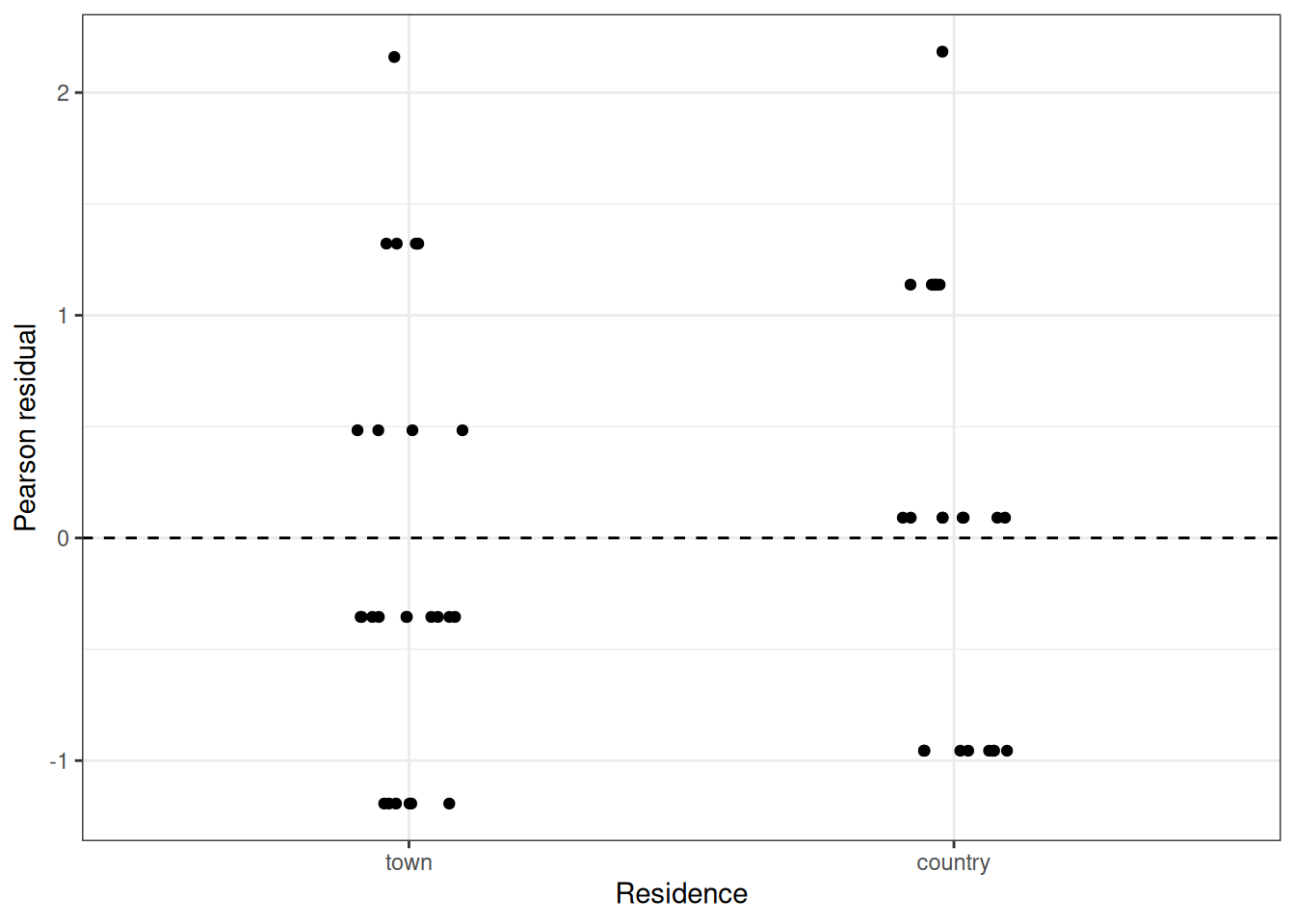
Figure 10 plots all 49 Pearson residuals. The largest residual in absolute value is 2.184, and the Pearson chi-squared statistic is \(X^2 \approx\) 43.66 on \(49 - 2 =\) 47 residual degrees of freedom, so \(X^2 / 47 \approx\) 0.929. No residual is extreme, and the ratio is below 1, so the data show no sign of more variability than the Poisson model allows.
Show R code
library(ggplot2)chronic$pearson<-r_pearsonggplot(chronic, aes(x =residence, y =pearson))+geom_hline(yintercept =0, linetype ="dashed")+geom_jitter(width =0.1, height =0)+labs(x ="Residence", y ="Pearson residual")+theme_bw()
Figure 10: Pearson residuals from the Poisson model for the chronic medical conditions data, by residence
10.5 Step 4: Inference
The final step is inference: Dobson and Barnett [10, Sec. 2.3.5] lists confidence intervals, hypothesis tests about the parameters, and interpretation of the results. By the central limit theorem for MLEs, in large samples \(\hat{\beta}\) is approximately Gaussian, with covariance matrix approximated by the inverse of the observed information\(-{\ell''\mathopen{}\left(\hat{\beta}\right)\mathclose{}}\). A 95% Wald confidence interval for \(\beta_j\) is then \(\hat{\beta}_j \pm 1.96 \cdot {\mathop{\widehat{\operatorname{SE}}}\nolimits\mathopen{}\left(\hat{\beta}_j\right)\mathclose{}}\), and the Wald statistic\(z_j \stackrel{\text{def}}{=}\hat{\beta}_j / {\mathop{\widehat{\operatorname{SE}}}\nolimits\mathopen{}\left(\hat{\beta}_j\right)\mathclose{}}\) tests \(H_0: \beta_j = 0\).
Example 25 (Comparing town and country women) In Example 22, the fitted means sum to \(\sum_{i:\, x_i = 0} \hat{\mu}_i = n_{\text{town}} \bar{y}_{\text{town}} = 37\) for the town women and \(\sum_{i:\, x_i = 1} \hat{\mu}_i = n_{\text{country}} \bar{y}_{\text{country}} = 21\) for the country women. Substituting into the Hessian from Example 23, the observed information matrix is
The lower-right entry is the estimated variance of \(\hat{\beta}_1\):
\[
\begin{aligned}
{\mathop{\widehat{\operatorname{Var}}}\nolimits\mathopen{}\left(\hat{\beta}_1\right)\mathclose{}}
&= \frac{58}{777}
\\
&= \frac{37 + 21}{37 \cdot 21}
&& \text{(} 58 = 37 + 21 \text{, } 777 = 37 \cdot 21 \text{)}
\\
&= \frac{1}{21} + \frac{1}{37}
&& \text{(distribute the division over the sum, then cancel the common factors)}
\\
&\approx 0.0746
\end{aligned}
\]
so \({\mathop{\widehat{\operatorname{SE}}}\nolimits\mathopen{}\left(\hat{\beta}_1\right)\mathclose{}} \approx \sqrt{0.0746} \approx 0.2732\).
Show R code
se_b1<-sqrt(1/21+1/37)ci_b1<-b1_hat+c(-1, 1)*qnorm(0.975)*se_b1z_b1<-b1_hat/se_b1p_b1<-2*pnorm(-abs(z_b1))summary(chronic_glm)$coefficients#> Estimate Std. Error z value Pr(>|z|)#> (Intercept) 0.352821 0.164399 2.14613 0.0318627#> country -0.443793 0.273214 -1.62434 0.1043026
The 95% Wald confidence interval for \(\beta_1\) is from -0.979 to 0.092.
Exponentiating the estimate and the interval endpoints, the estimated ratio of the country mean to the town mean is \({\operatorname{exp}\mathopen{}\left\{\hat{\beta}_1\right\}\mathclose{}} \approx\) 0.642, with 95% confidence interval from 0.376 to 1.096.
The Wald statistic is \(z \approx\) -1.624, with two-sided \(p\)-value\(\approx\) 0.104.
These hand calculations match the standard error, \(z\) value, and \(p\)-value that summary() reports for country. On average, country women in this sample reported 36% fewer chronic conditions than town women, but the confidence interval for the ratio includes 1, so these data are also consistent with no difference in the mean number of conditions.
11 Choosing a model
The choice of statistical model depends on several considerations, primary among which is the type of response variable.
Measured continuous values such as protein level, age, or weight can usually be modeled using linear regression, possibly after applying a logarithmic transformation.
If count data exhibit greater variance than assumed under the Poisson model, we can use negative binomial regression or overdispersed Poisson models.
Other outcome structures correspond to other families within the generalized linear model framework.
In generalized linear modeling, we specify a linear predictor\(\eta \stackrel{\text{def}}{=}\mathord{\smash[b]{\underset{\raise.3ex\hbox{$\scriptstyle\sim$}}{x}}\vphantom{x}}\cdot \mathord{\smash[b]{\underset{\raise.3ex\hbox{$\scriptstyle\sim$}}{\beta}}\vphantom{\beta}}\) of the same form as in linear regression. In principle, a linear predictor can yield any real value, whether positive, negative, or zero.
We then select an appropriate outcome distribution matched to the data type (for example, Gaussian for unbounded continuous values, gamma for positive continuous quantities, binomial for binary outcomes, and Poisson for counts).
Finally, we specify a link function\(g(\cdot)\) that maps the expected outcome \(\mu \stackrel{\text{def}}{=}{\mathbb{E}\mathopen{}\left[Y \mid \mathord{\smash[b]{\underset{\raise.3ex\hbox{$\scriptstyle\sim$}}{X}}\vphantom{X}}= \mathord{\smash[b]{\underset{\raise.3ex\hbox{$\scriptstyle\sim$}}{x}}\vphantom{x}}\right]\mathclose{}}\) onto the real line \((-\infty, \infty)\) of the linear predictor. The inverse link function \(g^{-1}(\cdot)\) transforms the linear predictor back to the scale of the expected outcome.
Standard linear regression uses the identity link function \(g(\mu) \stackrel{\text{def}}{=}\mu\) and assumes a Gaussian response distribution.
When predicting an inherently positive outcome, a log link function \(g(\mu) \stackrel{\text{def}}{=}{\operatorname{log}\mathopen{}\left\{\mu\right\}\mathclose{}}\) is often appropriate, since \({\operatorname{exp}\mathopen{}\left\{\eta\right\}\mathclose{}} > 0\) for all real \(\eta\).
An alternative to fitting a generalized linear model with a log link is to apply a log transformation directly to the outcome. While log-transforming the outcome works well for positive continuous measurements, it cannot be applied directly to binary outcomes or to count outcomes that can equal zero.
Table 5 lists the outcome families available in R’s glm() function, together with the link functions each family accepts (the default link for each family is in bold), and Table 6 defines each link function.
Table 5: Families and link functions available in R’s glm()
Family
Links
gaussian
identity, log, inverse
binomial
logit, probit, cauchit, log, cloglog
gamma
inverse, identity, log
inverse.gaussian
1/mu^2, inverse, identity, log
Poisson
log, identity, sqrt
quasi
identity, logit, probit, cloglog, inverse, log, 1/mu^2 and sqrt
quasibinomial
logit, probit, identity, cloglog, inverse, log, 1/mu^2 and sqrt
quasipoisson
log, identity, logit, probit, cloglog, inverse, 1/mu^2 and sqrt
Table 6: Link functions available in R’s glm(), where \(\eta \stackrel{\text{def}}{=}\mathord{\smash[b]{\underset{\raise.3ex\hbox{$\scriptstyle\sim$}}{x}}\vphantom{x}}\cdot \mathord{\smash[b]{\underset{\raise.3ex\hbox{$\scriptstyle\sim$}}{\beta}}\vphantom{\beta}}= g(\mu)\)
hospital length of stay (days), measured continuously
positive and right-skewed
gamma
log
For the last outcome, the canonical inverse link of the gamma family would also be allowed, but the log link keeps the fitted means positive for every value of the linear predictor and makes \({\operatorname{exp}\mathopen{}\left\{\beta_j\right\}\mathclose{}}\) a ratio of means, just as in Example 21.
Exercise 6 (Identifying GLM components) (adapted from Dobson and Barnett [10], Chapter 4, and Dunn and Smyth [9], Chapter 5)
For each of the following scenarios, identify the three components of the GLM: (1) the outcome distribution, (2) the link function \(g(\cdot)\), and (3) the linear predictor \(\eta = \mathord{\smash[b]{\underset{\raise.3ex\hbox{$\scriptstyle\sim$}}{x}}\vphantom{x}}\cdot \mathord{\smash[b]{\underset{\raise.3ex\hbox{$\scriptstyle\sim$}}{\beta}}\vphantom{\beta}}\).
(a) Modeling the probability of a binary outcome (disease/no disease) as a function of continuous predictors, using the logit link.
(b) Modeling count data (number of events per person-year) as a function of continuous predictors, using the log link.
(c) Modeling a continuous, strictly positive outcome using a gamma distribution and log link.
Exercise 7 (Canonical link functions) (adapted from Dobson and Barnett [10], Chapter 3, and Dunn and Smyth [9], Chapter 5)
The canonical link for a distribution in the exponential family is the link \(g(\cdot)\) such that \(g(\mu) = \theta\), where \(\theta\) is the natural parameter (see Canonical links).
For each listed distribution, state the canonical link function and the corresponding variance function \(V(\mu)\), where \({\operatorname{Var}\mathopen{}\left(Y\right)\mathclose{}} = \phi\, V(\mu)\) and \(\phi\) is the dispersion parameter:
(a)\(Y \sim \operatorname{Pois}(\mu)\)
(b)\(Y \sim \operatorname{Bernoulli}(\pi)\)
(c)\(Y \sim \operatorname{N}(\mu, \sigma^2)\)
(d)\(Y \sim \text{Gamma}(\mu, \phi)\), with mean \(\mu\) and shape \(1/\phi\)
For the Poisson distribution, the variance equals the mean. Overdispersion occurs when the empirical variance exceeds the mean.
For the Bernoulli distribution, the variance is maximized at \(\pi = 0.5\).
For the Normal distribution, the variance does not depend on the mean; the dispersion parameter \(\phi = \sigma^2\).
For the Gamma distribution, the coefficient of variation \({\operatorname{SD}\mathopen{}\left(Y\right)\mathclose{}}/{\mathbb{E}\mathopen{}\left[Y\right]\mathclose{}}\) is constant.
The sign of the Gamma canonical link is a convention: \(\theta = -1/\mu\) in the density’s natural parameterization, while R’s Gamma() family uses \(1/\mu\) as its default inverse link. Either way, the linear predictor can produce a negative \(\mu\).
The log link (not the canonical inverse link) is often used for Gamma regression in practice, because it ensures \(\mu > 0\) and gives interpretable multiplicative effects.
References
[1]
H. Wickham, M. Çetinkaya-Rundel, and G. Grolemund, R for data science. " O’Reilly Media, Inc.", 2023. Available: https://r4ds.hadley.nz/
E. Vittinghoff, D. V. Glidden, S. C. Shiboski, and C. E. McCulloch, Regression methods in biostatistics: Linear, logistic, survival, and repeated measures models, 2nd ed. Springer, 2012. Available: https://doi.org/10.1007/978-1-4614-1353-0
G. James, D. Witten, T. Hastie, and R. Tibshirani, An introduction to statistical learning: With applications in R, 2nd ed. Springer, 2021. doi: 10.1007/978-1-0716-1418-1.
[6]
J. Neyman, “On the application of probability theory to agricultural experiments. Essay on principles. Section 9,”Statistical Science, vol. 5, no. 4, pp. 465–472, 1990, doi: 10.1214/ss/1177012031.
[7]
D. B. Rubin, “Estimating causal effects of treatments in randomized and nonrandomized studies,”Journal of Educational Psychology, vol. 66, no. 5, pp. 688–701, 1974, doi: 10.1037/h0037350.
A. J. Dobson and A. G. Barnett, An introduction to generalized linear models, 4th ed. CRC press, 2018. Available: https://doi.org/10.1201/9781315182780
The “~” (“tilde”) symbol in the notation \(\mathord{\smash[b]{\underset{\raise.3ex\hbox{$\scriptstyle\sim$}}{X}}\vphantom{X}}\) indicates that \(\mathord{\smash[b]{\underset{\raise.3ex\hbox{$\scriptstyle\sim$}}{X}}\vphantom{X}}\) is a vector. See the notation page of the lab’s math notes for a table of notation used in these notes.↩︎
---title: "Introduction to GLMs"aliases: - glms.htmlformat: html: default revealjs: output-file: Intro-to-GLMs-slides.html pdf: output-file: Intro-to-GLMs-handout.pdf docx: output-file: Intro-to-GLMs-handout.docx---# Introduction{{< include shared-config.qmd >}}# WelcomeWelcome to Epidemiology 204: Quantitative Epidemiology III (Statistical Models).Epi 204 is a course on **regression modeling**. # What you should already know {.scrollable}{{< include prereq-knowledge.qmd >}}# What we will cover in this course* Linear (Gaussian) regression models (review and more details)* Regression models for non-Gaussian outcomes + binary + count + time to event* Statistical analysis using RWe will start where Epi 203 left off: with linear regression models.{{< include _subfiles/Intro-to-GLMs/_sec_outcome_types.qmd >}}# The scientific method and models{{< include _subfiles/Intro-to-GLMs/_sec_scientific_method.qmd >}}# Motivations for regression models:::{#exr-why-regression}Why do we need regression models?:::{{< slidebreak >}}::: {#sol-why-regression .incremental}* when there's not enough data to analyze every subgroup of interest individually* especially when subgroups are defined using continuous predictors:::---{{< include _subfiles/Intro-to-GLMs/_sec_regression_uses.qmd >}}## Example: Adelie penguins```{r}#| label: fig-palmer-1#| fig-cap: Palmer penguins#| echo: falselibrary(ggplot2)library(plotly)library(dplyr)ggpenguins <- palmerpenguins::penguins |> dplyr::filter(species =="Adelie") |>ggplot( ) +aes(x = bill_length_mm, y = body_mass_g) +geom_point() +xlab("Bill length (mm)") +ylab("Body mass (g)")print(ggpenguins)```## Linear regression```{r}#| label: fig-palmer-2#| fig-cap: Palmer penguins with linear regression fitggpenguins2 <- ggpenguins +stat_smooth(method ="lm",formula = y ~ x,geom ="smooth" )ggpenguins2 |>print()```## Curved regression lines```{r}#| label: fig-palmer-3#| fig-cap: Palmer penguins - curved regression linesggpenguins2 <- ggpenguins +stat_smooth(method ="lm",formula = y ~log(x),geom ="smooth" ) +xlab("Bill length (mm)") +ylab("Body mass (g)")ggpenguins2```## Multiple regression```{r}#| label: fig-palmer-4#| fig-cap: "Palmer penguins - multiple groups"ggpenguins <- palmerpenguins::penguins |>ggplot(aes(x = bill_length_mm,y = body_mass_g,color = species ) ) +geom_point() +stat_smooth(method ="lm",formula = y ~ x,geom ="smooth" ) +xlab("Bill length (mm)") +ylab("Body mass (g)")ggpenguins |>print()```## Modeling non-Gaussian outcomes::: {#fig-beetles_1a}```{r}library(glmx)data(BeetleMortality)beetles <- BeetleMortality |>mutate(pct = died / n,survived = n - died )plot1 <- beetles |>ggplot(aes(x =10^dose, y = pct)) +geom_point(aes(size = n)) +scale_x_log10(breaks =c(40, 50, 60, 70, 80, 100)) +xlab("Dose of CS2 (mg/L)") +ylab("Mortality rate (%)") +scale_y_continuous(labels = scales::percent) +scale_size(range =c(1, 2))print(plot1)```Mortality rates of adult flour beetles after five hours' exposure to gaseous carbon disulphide (Bliss 1935).The `dose` column holds the base-10 logarithm of the dose in mg/L,and the models use it as is;the figures show the dose itself, in mg/L, on a log-spaced axis.:::## Why don't we use linear regression?:::{#fig-beetles-plot1}```{r}beetles_long <- beetles |>reframe(.by =everything(),outcome =c(rep(1, times = died),rep(0, times = survived) ) )lm1 <- beetles_long |>lm(formula = outcome ~ dose,data = _ )f_linear <-function(x) predict(lm1, newdata =data.frame(dose =log10(x)))plot2 <- plot1 +geom_function(fun = f_linear, aes(col ="Straight line")) +labs(colour ="Model", size ="")print(plot2)```Mortality rates of adult flour beetles after five hours' exposure to gaseous carbon disulphide (Bliss 1935):::## Zoom out:::{#fig-beetles2}```{r}#| echo: falseprint(plot2 +expand_limits(x =c(40, 100)))```Mortality rates of adult flour beetles after five hours' exposure to gaseous carbon disulphide (Bliss 1935)::::## log transformation of dose?:::{#fig-beetles3}```{r}lm2 <- beetles_long |>lm(formula = outcome ~log(dose), data = _)f_linearlog <-function(x) predict(lm2, newdata =data.frame(dose =log10(x)))plot3 <- plot2 +expand_limits(x =c(40, 100)) +geom_function(fun = f_linearlog, aes(col ="Log-transform dose"))print(plot3 +expand_limits(x =c(40, 100)))```Mortality rates of adult flour beetles after five hours' exposure to gaseous carbon disulphide (Bliss 1935):::## Logistic regression:::{#fig-beetles4b}```{r}glm1 <- beetles |>glm(formula =cbind(died, survived) ~ dose, family ="binomial")f <-function(x) { glm1 |>predict(newdata =data.frame(dose =log10(x)), type ="response")}plot4 <- plot3 +geom_function(fun = f, aes(col ="Logistic regression"))print(plot4)```Mortality rates of adult flour beetles after five hours' exposure to gaseous carbon disulphide (Bliss 1935):::# Structure of regression models{{< include _subfiles/Intro-to-GLMs/_sec_regression_defs.qmd >}}{{< slidebreak >}}:::{#exr-glm-structure}What is the general structure of a generalized linear model?:::{{< slidebreak >}}:::{#sol-glm-structure}{{< include _subfiles/Intro-to-GLMs/_sec_glm_structure.qmd >}}:::{{< slidebreak >}}{{< include _subfiles/Intro-to-GLMs/_def-linear-predictor.qmd >}}{{< slidebreak >}}{{< include _subfiles/Intro-to-GLMs/_def-link-function.qmd >}}{{< slidebreak >}}{{< include _subfiles/Intro-to-GLMs/_def-outcome-distribution.qmd >}}{{< slidebreak >}}{{< include _subfiles/Intro-to-GLMs/_def-glm.qmd >}}{{< slidebreak >}}{{< include _subfiles/Intro-to-GLMs/_def-interaction.qmd >}}{{< slidebreak >}}{{< include _subfiles/Intro-to-GLMs/_def-interaction-term.qmd >}}{{< slidebreak >}}{{< include _subfiles/Intro-to-GLMs/_exm-interaction.qmd >}}# Why link functions? {#sec-why-link}{{< include _subfiles/Intro-to-GLMs/_sec_link_motivation.qmd >}}# Canonical links {#sec-canonical-link}{{< include _subfiles/Intro-to-GLMs/_sec_canonical_link.qmd >}}# The model fitting process {#sec-glm-fitting}The rest of this chapter is adapted from@dobson4e [Chapter 2].{{< include _subfiles/glms/_sec_model_fitting_process.qmd >}}{{< slidebreak >}}{{< include _subfiles/glms/_exm_chronic_eda.qmd >}}## Step 1: Model specification{{< include _subfiles/glms/_sec_specification.qmd >}}## Step 2: Parameter estimation{{< include _subfiles/glms/_sec_estimation.qmd >}}## Step 3: Checking model adequacy{{< include _subfiles/glms/_sec_checking.qmd >}}## Step 4: Inference{{< include _subfiles/glms/_sec_inference.qmd >}}# Choosing a model {#sec-choosing-glm}{{< include _subfiles/glms/_sec_choosing_model.qmd >}}---# Exercises {.unnumbered}{{< include _subfiles/Intro-to-GLMs/_exr-prac-glm-components.qmd >}}{{< slidebreak >}}{{< include _subfiles/Intro-to-GLMs/_exr-prac-canonical-link.qmd >}}# References {.unnumbered}::: {#refs}:::