2Neural Networks
Last modified: 2026-10-27
Source
Adapted from Brian Hutchinson’s Fall 2025 lecture notes, reorganized as exercises. The threshold neuron, its two diagrams, and the deep-network and autoencoder sketches come from Kameron Decker Harris’ 2022 Week 7 notes. The layer-counting convention, depth and width, and the region-counting argument for depth come from Logan Sizemore’s Spring 2025 lectures on representational power and on deep networks.
This chapter covers what a network can represent. We converted the source’s second half — training, minibatching, and back-propagation — in the back-propagation chapter, where it belongs and where the source itself defers it (“will come back to this”). We kept the unsplit original as an outtake in this page’s source. We kept the polished derivation this chapter carried before the rebuild, and the “Training deep networks” material (vanishing, exploding and shattered gradients; residual connections; choosing the hidden non-linearity), as an outtake too. The back-propagation chapter has since converted the substance of the training material: vanishing, exploding and shattered gradients, the rectified linear unit (ReLU) remedy, residual connections and choosing the hidden non-linearity.
We do not repeat the source’s cross-entropy and maximum-likelihood derivations here, since logistic regression already works them; Exercise 86 cross-references them instead.
We qualify one claim rather than reproduce it. The source says an arbitrary logic function “may require \(O(2^{\ninputvars})\) hidden nodes”, the cost of the disjunctive normal form (DNF) construction. Exercise 68 builds that construction, and then shows that parity — the standard example of a hard Boolean function — needs only \(\ninputvars\) units.
1 When a line is not enough
Linear regression fits a hyperplane and logistic regression separates with one. Both are useful far beyond what their simplicity suggests, and both stop at the same limit: the boundary they draw is flat.
Plenty of problems are not flat. Which object a grid of pixels shows depends on colour, rotation and lighting together; which speech sound a spectrum encodes depends on the speaker’s age, their vocal tract and the microphone at once. In each case the quantity you want is a complicated function of the measurements you have, and no weighting of those measurements recovers it.
There are three ways to go beyond a flat boundary, and this chapter is about the third.
- Map the features into a new space with a transform you choose. This is a basis expansion.
- Map them into a new space with a transform you never write down. This is the kernel trick, and it belongs to support vector machines.
- Learn the transform from the data. This is a neural network.
The first is the cheapest to understand and the most expensive to run, so it makes the right starting point.
Exercise 1 (Three ways out of a straight line)
Exercise 1 (Three ways out of a straight line) Every model in these notes so far draws a straight boundary, or a boundary made of straight pieces. Logistic regression is the clearest case: its boundary is the hyperplane \(\dprod{\vcoef}{\vx} = 0\).
The exclusive-or (XOR) data of the decision boundary exercise has a point of each class in each of two opposite quadrants. Say in one sentence why no choice of \(\vcoef\) classifies all four points, and why this is a statement about the model rather than about the fitting algorithm.
Solution 1. A linear model assigns \(\hy = 1\) exactly on one side of a hyperplane. The XOR circles sit at \((-1, 1)\) and \((1, -1)\) and the crosses at \((1,1)\) and \((-1,-1)\), so each class occupies two opposite quadrants. Any line through the plane leaves the two opposite quadrants on the same side or splits both of them, so no line has all circles on one side.
This is a statement about the model because the failure holds for every \(\vcoef\) at once, not for the particular \(\vcoef\) some algorithm happened to return. A better optimizer, more iterations or a different starting point change nothing: the function class does not contain a separator. The distinction matters because the two failures look identical from the outside — a fit that does not classify the training data — and they have opposite remedies.
Exercise 2 (Three ways out of a straight line (part 2))
Exercise 2 (Three ways out of a straight line (part 2)) Use the setup of Exercise 1.
Suppose you are allowed to invent one new feature, computed from \(\predvar_1\) and \(\predvar_2\), and then fit a linear model in the enlarged feature vector. Give a feature that makes XOR linearly separable, and give the \(\vcoef\) that separates it.
Solution 2. Take \(x_3 = x_1 x_2\). The class is the sign of \(x_1 x_2\): the crosses have \(x_3 = 1\) and the circles have \(x_3 = -1\). So \(\vcoef = \pt{0, 0, 0, 1}\), reading the coefficients as \((\coef{0}, \coef{1}, \coef{2}, \coef{3})\), gives \(\dprod{\vcoef}{\vx} = x_1x_2\), which is positive on exactly the crosses.
The boundary in the enlarged space is the hyperplane \(\predvar_3 = 0\). Pulled back to the original plane it is the set \(x_1 x_2 = 0\), which is the pair of axes — not a line. A linear boundary in the enlarged space is a curved one in the original space, and that is the whole idea.
Exercise 3 (Three ways out of a straight line (part 3))
Exercise 3 (Three ways out of a straight line (part 3)) Use the setup of Exercise 1.
Exercise 2 is the whole idea of this chapter in miniature. Three strategies follow from it, and they differ in who chooses the new features:
- a fixed transform you write down yourself;
- a fixed transform you never write down, used only through inner products;
- a transform whose parameters are fitted alongside everything else.
Name the method this course attaches to each, and say which one requires you to know in advance which features matter.
Solution 3.
| who chooses the features | method | needs advance knowledge? |
|---|---|---|
| you write the transform down | basis expansion | yes |
| the transform is implicit, used only through inner products | kernels and SVMs | partly: you choose the kernel |
| the transform is fitted | neural networks | no |
Basis expansion is the one that needs you to know which features matter. You must commit to \(\vfeatmap\) before seeing how well it works, and Exercise 8 shows that guarding against a wrong choice by including everything is expensive.
Proof
Proof. By Solution 1.
Theorem 2 (The product feature separates XOR)
Theorem 2 (The product feature separates XOR) Add the feature \(x_3 = x_1 x_2\) to the four XOR points of Theorem 1. In the enlarged feature space, \(\vcoef = \pt{0, 0, 0, 1}\) classifies all four points correctly, with boundary the hyperplane \(x_3 = 0\). In the original plane that boundary is the set \(x_1 x_2 = 0\), the pair of axes.
Proof
Proof. By Solution 2.
Example 2 (The score with the product feature)
Example 2 (The score with the product feature) Add \(x_3 = x_1 x_2\) and score the four points with \(\vcoef = \pt{0, 0, 0, 1}\):
The scores are positive for the first two points and negative for the last two, which separates the classes.
2 Basis expansion
Adding \(x_1x_2\) by hand solved the problem in Exercise 1. The obvious generalization is to stop choosing and add everything: every product of the input coordinates up to some degree.
Exercise 4 (Write the expansion out)
Exercise 4 (Write the expansion out) A basis expansion replaces \(\vx\) by a vector of functions of \(\vx\):
\[\vfeatmap(\vx) = \begin{bmatrix} 1 \\ f_1(\vx) \\ \vdots \\ f_{\nparams}(\vx)\end{bmatrix}\]
and then fits an ordinary linear model in \(\vfeatmap(\vx)\) instead of \(\vx\). The \(L\)th-order polynomial expansion takes the \(f_j\) to be every monomial in \(x_1, \ldots, x_{\ninputvars}\) of total degree at most \(L\).
Write \(\vfeatmap(\vx)\) in full for \(\ninputvars = 1\), \(L = 3\).
Solution 4. \(\ninputvars = 1\), \(L = 3\):
\[\vfeatmap(x) = \begin{bmatrix} 1 \\ x_1 \\ x_1^2 \\ x_1^3 \end{bmatrix}\]
Four entries: one of each degree from \(0\) to \(3\).
Exercise 5 (Write the expansion out (part 2))
Exercise 5 (Write the expansion out (part 2)) Use the setup of Exercise 4.
Write it in full for \(\ninputvars = 2\), \(L = 2\). Be careful to list the first-order terms separately; a source that writes a single \(\predvar\) in this list means both \(\predvar_1\) and \(\predvar_2\).
Solution 5. \(\ninputvars = 2\), \(L = 2\):
\[\vfeatmap(\vx) = \begin{bmatrix} 1 \\ x_1 \\ x_2 \\ x_1^2 \\ x_2^2 \\ x_1 x_2 \end{bmatrix}\]
Six entries: one of degree \(0\), two of degree \(1\), three of degree \(2\). We easily drop the cross term \(\predvar_1\predvar_2\), and it carries the interaction, so we should check for it.
Exercise 6 (Write the expansion out (part 3))
Exercise 6 (Write the expansion out (part 3)) Use the setup of Exercise 4.
Write it in full for \(\ninputvars = 2\), \(L = 3\), and check your list against a count you can make without writing anything down: the number of monomials of total degree exactly \(k\) in \(2\) variables is \(k + 1\).
Solution 6. \(\ninputvars = 2\), \(L = 3\) adds the four monomials of degree exactly \(3\):
\[\vfeatmap(\vx) = \begin{bmatrix} 1 \\ x_1 \\ x_2 \\ x_1^2 \\ x_2^2 \\ x_1 x_2 \\ x_1^3 \\ x_2^3 \\ x_1^2 x_2 \\ x_1 x_2^2 \end{bmatrix}\]
Ten entries, and the count confirms it: degrees \(0, 1, 2, 3\) contribute \(1 + 2 + 3 + 4 = 10\). Getting the degree-\(3\) block right means remembering \(\predvar_1^2\predvar_2\) and \(\predvar_1\predvar_2^2\) as well as the two pure cubes — the same omission as in Solution 5, one degree up.
Exercise 7 (Write the expansion out (part 4))
Exercise 7 (Write the expansion out (part 4)) Use the setup of Exercise 4.
Nothing forces the \(f_j\) to be polynomials. Give an expansion suited to a feature that is strictly positive and spans several orders of magnitude, and one suited to a feature you expect to act periodically, such as hour of the day.
Solution 7. For a strictly positive feature spanning orders of magnitude, use \(\log x\), alone or alongside \(x\). A linear model in \(\log \predvar\) says the response is linear in the number of doublings rather than in the raw amount, which is usually the claim you actually believe about income, population or concentration. A cubic in the raw feature cannot express that and will use its flexibility mostly to fit the largest values.
For an hour-of-day feature, use \(\sin(2\pi x/24)\) and \(\cos(2\pi x/24)\). The point is continuity where the day ends and starts again: hour \(23\) and hour \(0\) are one hour apart, and every polynomial in \(\predvar\) makes them \(23\) apart. Adding the pair also builds in the period, which the data then does not have to use degrees of freedom to rediscover.
Adding everything works, and the drawback appears immediately.
Exercise 8 (Count the cost of hedging)
Exercise 8 (Count the cost of hedging) Exercise 4 asks you to commit to a transform before you know which features matter. The obvious precaution is to include everything up to some order. This exercise computes the cost of that precaution.
How many monomials of total degree exactly \(k\) are there in \(\ninputvars\) variables? Derive the count rather than quoting it: a monomial \(\predvar_1^{a_1}\cdots \predvar_{\ninputvars}^{a_{\ninputvars}}\) of degree \(k\) is a choice of non-negative integers \(a_1, \ldots, a_{\ninputvars}\) summing to \(k\), so count those.
Solution 8. Count the solutions of \(a_1 + \cdots + a_{\ninputvars} = k\) in non-negative integers. Lay out \(k\) identical tokens in a row and insert \(\ninputvars - 1\) dividers among them; the tokens before the first divider give \(a_1\), those between the first and second give \(a_2\), and so on. Every arrangement of \(k\) tokens and \(\ninputvars-1\) dividers gives exactly one solution and every solution gives exactly one arrangement, so the count is the number of ways to choose which \(k\) of the \(k + \ninputvars - 1\) positions hold tokens:
\[\#\{\text{degree exactly } k\} = \binom{k + \ninputvars - 1}{k}\]
Check it at \(\ninputvars = 2\): \(\binom{k+1}{k} = k+1\), which is the count used in Exercise 6.
Exercise 9 (Count the cost of hedging (part 2))
Exercise 9 (Count the cost of hedging (part 2)) Use the setup of Exercise 8.
Sum over \(k = 0, \ldots, L\) to get \(\nparams\), the length of \(\vfeatmap(\vx)\), and simplify to a single binomial coefficient.
Solution 9. Summing over \(k\) and using the hockey-stick identity \(\sum_{k=0}^{L}\binom{k + \ninputvars - 1}{k} = \binom{L + \ninputvars}{L}\):
\[\nparams = \binom{\ninputvars + L}{L}\]
We can derive the identity directly instead of looking it up. Choosing \(L\) items from \(\ninputvars + L\) is the same as deciding how many of the first few you skip, and grouping the choices by that number reproduces the sum term by term.
Check against Exercise 4: \(\binom{4}{3} = 4\), \(\binom{4}{2} = 6\), \(\binom{5}{3} = 10\), matching the three lists written out there.
Exercise 10 (Count the cost of hedging (part 3))
Exercise 10 (Count the cost of hedging (part 3)) Use the setup of Exercise 8.
Evaluate your formula at \(\ninputvars = 100\) for \(L = 2\) and \(L = 3\).
Solution 10. \[ \begin{aligned} \binom{102}{2} &= \frac{102 \cdot 101}{2} \\ &= 5151, \end{aligned} \qquad \begin{aligned} \binom{103}{3} &= \frac{103 \cdot 102 \cdot 101}{6} \\ &= 176{,}851 \end{aligned} \]
A hundred features become five thousand, or a hundred and seventy-seven thousand.
Exercise 11 (Count the cost of hedging (part 4))
Exercise 11 (Count the cost of hedging (part 4)) Use the setup of Exercise 8.
Show that for fixed \(L\) your answer grows like \(\ninputvars^L/L!\) as \(\ninputvars \to \infty\), which is the precise form of the claim that a second-order expansion costs \(O(\ninputvars^2)\) and a third-order one \(O(\ninputvars^3)\).
Solution 11. Write the binomial out:
\[\binom{\ninputvars+L}{L} = \frac{(\ninputvars+L)(\ninputvars+L-1)\cdots(\ninputvars+1)}{L!}\]
The numerator is a product of \(L\) factors, each of which is \(\ninputvars\) plus a constant, so it equals \(\ninputvars^L(1 + O(1/\ninputvars))\). Hence \(\nparams \sim \ninputvars^L/L!\) with \(L\) held fixed.
At \(\ninputvars = 100\), \(L = 3\) the approximation gives \(10^6/6 \approx 166{,}667\) against the exact \(176{,}851\) — close, and an underestimate, as it must be since every discarded factor exceeds \(\ninputvars\).
Note what the statement does not say. The growth is polynomial in \(\ninputvars\) for fixed \(L\), and exponential in \(L\) for fixed \(\ninputvars\). “\(O(\ninputvars^3)\)” is a claim about widening the feature vector, not about raising the order.
Exercise 12 (Count the cost of hedging (part 5))
Exercise 12 (Count the cost of hedging (part 5)) Use the setup of Exercise 8.
A common guideline asks for several times more training points than parameters. Using Exercise 10, say what a third-order expansion of \(100\) features would demand, and connect this to the bias–variance decomposition: which term does an expansion like this reduce, and which does it inflate?
Solution 12. At \(\ninputvars = 100\), \(L = 3\) there are \(176{,}851\) parameters, so the guideline asks for something on the order of a million labelled examples to fit a cubic in a hundred features. Very few problems supply that.
In bias–variance terms the expansion enlarges the function class, so it can only reduce bias: the best attainable function is now at least as good as before, since the old class sits inside the new one. What it inflates is variance. Each additional parameter is one more quantity estimated from the same fixed sample, so the fitted function moves more from one training set to the next, which is overfitting.
This chapter exists to avoid that difficulty. Basis expansion gains expressiveness by adding parameters you chose in advance and cannot revise. A neural network fixes the number of parameters first — through the width \(L\) — and then fits the transform, so expressiveness and parameter count are no longer the same thing.
Theorem 3 (Number of polynomial features)
Theorem 3 (Number of polynomial features) For a polynomial in \(\ninputvars\) variables, the number of monomials of degree at most \(L\), including the constant \(1\), is
\[\nparams = \binom{\ninputvars + L}{L}.\]
For fixed \(L\), \(\nparams \sim \ninputvars^L / L!\) as \(\ninputvars \to \infty\).
Proof
Proof. By Solution 8, 2 and 4.
Before moving on, we state what a basis expansion does and does not change.
Exercise 13 (Why the old machinery still works)
Exercise 13 (Why the old machinery still works) A basis expansion looks like it should break least squares: the fitted function \(\modmemf{\vx} = \tp{\vw} \vfeatmap(\vx)\) is a cubic in \(\vx\), and nothing about a cubic is linear.
Say precisely which variables the model is linear in, and why that is the only linearity least squares ever required.
Solution 13. The model is linear in the parameters \(\vw\), not in the inputs. Least squares never asked for linearity in \(\vx\): the normal equations come from differentiating \(\hat R\) with respect to \(\vw\) and setting the result to zero, and that calculation sees \(\vfeatmap(\vx_i)\) only as a fixed vector of numbers.
Whether those numbers arose as \(x_i\), \(x_i^3\) or \(\sin x_i\) is invisible to the optimization. The phrase “linear model” is about the parameters throughout, and reading it as a claim about the shape of the fitted curve is a common and costly misreading.
Exercise 14 (Why the old machinery still works (part 2))
Exercise 14 (Why the old machinery still works (part 2)) Use the setup of Exercise 13.
Let \(\design\) be the \(\nobs \times \nparams\) matrix whose \(i\)th row is \(\vfeatmap\pt{\vx_i}\). Express the empirical risk \(\hat R(\vw)\) in matrix form and give the normal equations, quoting the normal-equations exercise rather than re-deriving them.
Solution 14. With \(\design \in \reals^{n \times \nparams}\) and \(\vy \in \reals^n\),
\[\hat R(\vw) = \frac{1}{n}\norm{ \vy - \design\vw }^2\]
and the normal equations are
\[\stprod{\design}\,\vw = \tp{\design} \vy\]
identical in form to the ordinary case with \(\design\) in place of \(X\).
Exercise 15 (Why the old machinery still works (part 3))
Exercise 15 (Why the old machinery still works (part 3)) Use the setup of Exercise 13.
State the condition under which those equations have a unique solution, in terms of \(\design\) rather than \(\design(\mx)\). Then give a concrete expansion, on data you choose, that violates it — so the failure is a property of the transform and not of the data being unlucky.
Solution 15. The solution is unique if and only if \(\stprod{\design}\) is invertible, which holds if and only if \(\design\) has full column rank \(\nparams\) (\(\tp{\design}\design\) is invertible exactly when \(\design\) has full column rank). Two things can break it, and the expansion itself creates the second.
Too few points. \(\design\) has \(n\) rows, so its rank is at most \(n\). Since \(\nparams\) grows as Theorem 3 shows, \(\nparams > n\) is easy to reach: a cubic in two features already needs \(\nobs \ge 10\).
A dependency among the columns, at any \(n\). Take \(\ninputvars = 2\) and a dataset in which \(x_2 = 2x_1\) for every point. Then in the second-order expansion the column for \(x_1x_2\) equals twice the column for \(x_1^2\), and the column for \(x_2^2\) equals four times it. \(\design\) has rank at most \(4\) however many points you collect, because the dependency is between the columns rather than a shortage of rows.
The contrast is the point of the part. Collecting more data fixes the first and never fixes the second.
Exercise 16 (Why the old machinery still works (part 4))
Exercise 16 (Why the old machinery still works (part 4)) Use the setup of Exercise 13.
Parts 1–3 hold for logistic regression too, with \(\vfeatmap(\vx_i)\) in place of \(\vx_i\). Say what the decision boundary of that model looks like in the original feature space, and check your answer against Solution 2.
Solution 16. The boundary is the set where \(\tp{\vw}\vfeatmap(\vx) = 0\). In the enlarged space that is a hyperplane; in the original feature space it is the zero set of a degree-\(L\) polynomial — a conic for \(L = 2\), a cubic curve for \(L = 3\), and in general a curved surface rather than a flat one.
Theorem 2 is the smallest instance: the single added feature \(x_3 = x_1x_2\) with \(\vw = \pt{0,0,0,1}\) gives the hyperplane \(x_3 = 0\) in the enlarged space, which pulls back to \(x_1x_2 = 0\), the two axes. Flat in the enlarged space, curved in the original space, and fitted by exactly the machinery of the previous two chapters.
Watch
Hutchinson covers nonlinear predictions by feature transformation (10 min) [2]. The video site requires a login, which enrolled students find in the syllabus.
3 Learning the features instead
A basis expansion fixes the features before it sees the data, and keeps every one it did not need. The alternative is to fix only how many features there will be, and let the fit decide what they are.
Write \(L\) for that number. The network computes
\[\vhidval = f\paren{\tp{W} \begin{bmatrix}1 \\ \vx\end{bmatrix}}, \qquad \vy = g\paren{\tp{U} \begin{bmatrix}1 \\ \vhidval\end{bmatrix}}, \tag{1}\]
where \(f\) is applied coordinate by coordinate and \(g\) depends on the task. \(\vhidval\) is the hidden layer: \(L\) features, computed from the input, with \(W\) fit alongside everything else.
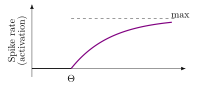
Each coordinate of \(\vhidval\) is a unit modelled on a neuron. A single artificial neuron computes a weighted sum of its inputs and fires when that sum passes a threshold:
\[y = f\paren{\sumto{i}{\ninputvars} w_i x_i - \unitthresh} \tag{2}\]
where \(\ninputvars\) is the number of inputs and \(f\) is a non-linear activation, which fires above the threshold \(\unitthresh\) (Figure 1).
Read
GeeksforGeeks explains the perceptron [3], a single threshold unit.
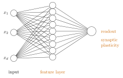
Stacking a layer of \(L\) such units gives a vector of features (Figure 2). Each unit carries its own weights and its own threshold, so both are indexed by \(i\):
\[\featmap_i = f\paren{\dprod{\vw_i}{\vx} - \unitthresh_i}, \qquad i = 1, \dots, L \tag{3}\]
and combining them is linear or non-linear depending on whether a second activation is applied:
\[\left. \begin{aligned} y &= \sumto{i}{L} \featmap_i(\vx)\,\coef{i} + \coef{0} \\ y &= \dprod{\vfeatmap}{\vcoef} + \coef{0} \end{aligned} \right\} \textcolor{orange}{\text{Linear}} \tag{4}\]
\[y = g\paren{\dprod{\vfeatmap}{\vcoef} + \coef{0}} \Big\} \textcolor{orange}{\text{Non-linear}}\]
Exercise 17 (From a threshold to a bias)
Exercise 17 (From a threshold to a bias) Equation 2 writes a unit with an explicit threshold \(\unitthresh\), and Equation 3 gives each of the \(L\) units its own weights \(\vw_i\) and its own threshold \(\unitthresh_i\). The network of Equation 1 has no \(\unitthresh\) anywhere.
Show that \(f\paren{\sumto{i}{\ninputvars} w_i \predvar_i - \unitthresh}\) is a unit of the form \(f(\dprod{\vw}{\vx})\), with \(\vx \in \reals^{\ninputvars+1}\) carrying a constant \(1\) in its first position.
Solution 17. Put the threshold in front of the weights, with its sign flipped:
\[\sumto{i}{\ninputvars} w_i x_i - \unitthresh = \begin{bmatrix} -\unitthresh \\ \vw \end{bmatrix}^\top \begin{bmatrix} 1 \\ \vx \end{bmatrix}.\]
Exercise 18 (From a threshold to a bias (part 2))
Exercise 18 (From a threshold to a bias (part 2)) Use the setup of Exercise 17.
What is the weight on that constant?
Solution 18. The weight on the constant is \(-\unitthresh\). A threshold and a bias are one parameter under two names: the unit fires when the weighted sum exceeds \(\unitthresh\), which is when the weighted sum with the bias included, called the pre-activation, is positive. These notes use the bias, written \(w_0\) for a single unit and stored in the row of \(W\) that multiplies the constant. Sources that start from the neuron write the threshold, as Equation 2 does.
Exercise 19 (From a threshold to a bias (part 3))
Exercise 19 (From a threshold to a bias (part 3)) Use the setup of Exercise 17.
The linear readout of Equation 4 reads a vector of features. Which model of this chapter is it when the \(\featmap_i\) are fixed in advance?
Solution 19. With the \(\featmap_i\) fixed in advance, the readout is a linear model in a chosen set of features, which is a basis expansion (Exercise 4).
Exercise 20 (From a threshold to a bias (part 4))
Exercise 20 (From a threshold to a bias (part 4)) Use the setup of Exercise 17.
Which model of this chapter is it when their weights and thresholds are fitted?
Solution 20. With their weights and thresholds fitted, it is the network of Equation 1 with \(g\) the identity and \(C = 1\).
Exercise 21 (From a threshold to a bias (part 5))
Exercise 21 (From a threshold to a bias (part 5)) Use the setup of Exercise 17.
Say which entries of \(W\) and \(U\) the \(\unitthresh_i\), the \(\coef{i}\) and \(\coef{0}\) become.
Solution 21. \(\vw_i\) and \(-\unitthresh_i\) form column \(i\) of \(W\), the \(\coef{i}\) are the entries of \(U\)’s single column that multiply \(\hidvalof{1}, \ldots, \hidvalof{L}\), and \(\coef{0}\) is the entry that multiplies the constant. The two models differ only in whether the features are written down or fitted.
Exercise 22 (Read the shapes off the diagram)
Exercise 22 (Read the shapes off the diagram) With one hidden layer (Figure 3), the computation is two matrix multiplications with a function applied between them:
\[\vhidval = f\paren{\tp{W} \vx}, \qquad \vy = g\paren{\tp{U} \begin{bmatrix} 1 \\ \vhidval\end{bmatrix}}\]
Here \(\vx \in \reals^{\ninputvars+1}\) carries a constant \(1\) in its first position, \(\vhidval \in \reals^{L}\) is the hidden layer whose entries are called units or neurons, and \(\vy \in \reals^{C}\) is the output. \(f\) and \(g\) are the activation functions, applied elementwise in the case of \(f\).
Read the diagram to give the shapes of \(W\) and \(U\), and say where each \(+1\) comes from.
Solution 22. \(W \in \reals^{(\ninputvars+1)\times L}\) and \(U \in \reals^{(L+1)\times C}\).
\(\tp{W}\vx\) must be a vector of length \(L\), and \(\vx\) has length \(\ninputvars+1\), so \(\tp{W}\) is \(L \times (\ninputvars+1)\) and \(W\) is its transpose. The \(+1\) in \(\ninputvars+1\) is the constant placed first in the input; the \(+1\) in \(L+1\) is the constant placed in front of \(\vhidval\). Each supplies a bias, so that a layer computes an affine function rather than one forced through the origin.
Exercise 23 (Read the shapes off the diagram (part 2))
Exercise 23 (Read the shapes off the diagram (part 2)) Use the setup of Exercise 22.
Give a formula for the total number of parameters.
Solution 23. \[\#\text{parameters} = (\ninputvars+1)L + (L+1)C\]
Exercise 24 (Read the shapes off the diagram (part 3))
Exercise 24 (Read the shapes off the diagram (part 3)) Use the setup of Exercise 22.
Evaluate it for \(\ninputvars = 784\), \(L = 100\), \(C = 10\).
Solution 24. At \(\ninputvars = 784\), \(L = 100\), \(C = 10\):
\[ \begin{aligned} 785 \times 100 + 101 \times 10 &= 78{,}500 + 1{,}010 \\ &= 79{,}510 \end{aligned} \]
Exercise 25 (Read the shapes off the diagram (part 4))
Exercise 25 (Read the shapes off the diagram (part 4)) Use the setup of Exercise 22.
Which of the two matrices holds almost all of them?
Solution 25. \(W\) holds \(98.7\%\) of them. That is the usual situation, and it says where the modelling capacity sits: almost the whole network is the map from raw inputs to learned features, and the classifier that uses those features has few parameters. Comparing \(78{,}500\) with the \(176{,}851\) of Solution 8’s cubic in a hundred features is the argument for this chapter in one line.
Exercise 26 (Read the shapes off the diagram (part 5))
Exercise 26 (Read the shapes off the diagram (part 5)) Use the setup of Exercise 22.
Write \(\outvar_c\), a single output coordinate, as an explicit double sum over the entries of \(W\) and \(U\). Written this way you can see each individual parameter, which the matrix form hides.
Solution 26. With \(f\) applied elementwise and \(U_{0c}\) the bias row,
\[y_c = g\paren{U_{0c} + \sum_{j=1}^{L} U_{jc}\, f\paren{\sum_{d=0}^{\ninputvars} W_{dj}\, x_d}}\]
writing \(\predvar_0 = 1\) for the input’s constant. Every parameter appears exactly once, \(W_{dj}\) inside the activation and \(U_{jc}\) outside it. Because of that asymmetry, fitting the two matrices is not the same problem twice: a change to \(U\) acts on the output directly, while a change to \(W\) has to pass through \(f\) first.
Exercise 27 (Read the shapes off the diagram (part 6))
Exercise 27 (Read the shapes off the diagram (part 6)) Use the setup of Exercise 22.
The task dictates the choice of \(g\). Say which \(g\) you would use for a regression problem, for a two-class problem, and for a \(C\)-class problem, and in each case say what constraint on \(\vy\) that choice enforces.
Solution 27.
| task | \(g\) | constraint on \(\vy\) |
|---|---|---|
| regression | identity, \(g(z) = z\) | none: any real vector |
| two classes | logistic \(\sigmoid\) | a single number in \((0,1)\) |
| \(C\) classes | softmax | non-negative, summing to \(1\) |
The constraint is the reason for the choice in each case. A regression target is unbounded, so any squashing function would cap the prediction at a value the data can exceed. A two-class output must be a probability. A \(C\)-class output must be a probability distribution, and softmax enforces the sum rather than merely bounding each coordinate — \(C\) separate sigmoids bound each one and do not make them sum to \(1\).
Exercise 28 (Read the shapes off the diagram (part 7))
Exercise 28 (Read the shapes off the diagram (part 7)) Use the setup of Exercise 22.
Suppose you drop the constant \(1\) from the bracket in the second equation, so that \(U \in \reals^{L \times C}\). Describe a function the network can no longer represent, and connect this to the role of \(\coef{0}\) in logistic regression.
Solution 28. Without the constant \(1\), the output is \(g(\tp{U}\vhidval)\), which is \(g(0)\) whenever \(\vhidval = \vzero\). So the network can no longer set its output freely when the hidden layer is silent: with \(g\) the softmax, a zero hidden layer forces the uniform distribution, and the network cannot learn an unequal base rate for the classes.
This is the role of \(\coef{0}\) exactly. In logistic regression the intercept shifts the surface without rotating or scaling it, and removing it forces the boundary through the origin. Here \(U_{0c}\) shifts each output, and removing it forces the network to route every departure from \(g(\vzero)\) through the hidden units — using learned features for something a single parameter would supply.
Theorem 4 (Parameters of a one-hidden-layer network)
Theorem 4 (Parameters of a one-hidden-layer network) A network with \(\ninputvars\) inputs, \(L\) hidden units and \(C\) outputs, with a constant input to the hidden layer and a constant feeding the output layer, has \(W \in \reals^{(\ninputvars+1)\times L}\), \(U \in \reals^{(L+1)\times C}\) and
\[(\ninputvars+1)L + (L+1)C\]
parameters.
Proof
Proof. By Solution 22.
Counting layers
The network of Equation 1 has an input layer, a hidden layer and an output layer, so some sources call it a three-layer network. These notes call it a two-layer network instead, counting the two weight matrices — input-to-hidden and hidden-to-output — rather than the three rows of units, or say that it has one hidden layer. The notation choices page gives the reason for counting this way. Both names are in use, so check which one a source means before comparing depths.
This network — \(\vhidval = f\paren{\tp{W}[1; \vx]}\) and \(\vy = g\paren{\tp{U}[1; \vhidval]}\) — contains logistic regression as a special case, which we check explicitly before going further.
Exercise 29 (Find the models you already know)
Exercise 29 (Find the models you already know) Take \(f = \sigmoid\) and \(g = \mathrm{softmax}\) in Exercise 22.
Set \(L = \ninputvars\) and \(W = I\), the identity, so the hidden layer copies the input unchanged. Show that the network reduces to multinomial logistic regression, and say which of \(W\) and \(U\) plays the part of the coefficient matrix \(B\).
Solution 29. With \(W = I\) the pre-activation is \(\vx\) itself, so \(\vhidval = \sigmoid(\vx)\) — elementwise, and note this is not quite the raw input, a point Solution 32 returns to. The output is then
\[\vy = \mathrm{softmax}\paren{\tp{U}\begin{bmatrix}1 \\ \vhidval\end{bmatrix}}\]
which is exactly the multinomial logistic regression of the softmax exercise with \(B = U\): one column of \(U\) per class, each giving that class’s score as a linear function of the features, passed through softmax.
So \(U\) plays the part of \(B\). \(W\) has no counterpart in logistic regression at all.
Exercise 30 (Find the models you already know (part 2))
Exercise 30 (Find the models you already know (part 2)) Use the setup of Exercise 29.
Now take \(C = 1\) with \(g = \sigmoid\) instead. Under the same choice of \(W\), which model is this, and what is \(\vcoef\)?
Solution 30. \(C = 1\) with \(g = \sigmoid\) is ordinary two-class logistic regression, and \(\vcoef\) is the single column of \(U\) — its bias entry \(U_{01}\) is \(\coef{0}\) and the remaining \(L\) entries are the slopes.
The one thing to check is the label convention: a single output through \(\sigmoid\) models \(P(Y = 1 \mid \vx)\) directly, matching the \(0/1\) convention rather than the \(\pm 1\) margin form.
Exercise 31 (Find the models you already know (part 3))
Exercise 31 (Find the models you already know (part 3)) Use the setup of Exercise 29.
Parts 1 and 2 put the familiar model on top of the hidden layer. Say in one sentence what the network is therefore doing that logistic regression cannot, and why the phrase “learned features” describes it.
Solution 31. The network applies logistic regression to a representation it has learned, instead of to the features it was given. Logistic regression’s boundary is linear in whatever it is given, and that is not a limitation the network shares, because \(W\) is fitted: the network can move the data into a space where a linear boundary works, and choose that space using the labels.
“Learned features” is the right phrase because \(\vhidval\) occupies the same position in the model that \(\vfeatmap(\vx)\) occupies in Exercise 4 — a vector of derived quantities the classifier reads — with the difference that \(\vfeatmap\) was written down in advance and \(\vhidval\) is estimated.
Exercise 32 (Find the models you already know (part 4))
Exercise 32 (Find the models you already know (part 4)) Use the setup of Exercise 29.
\(W = I\) needs \(L = \ninputvars\). Explain why a network with \(L \neq \ninputvars\) still contains a logistic regression as a special case whenever \(L \geq \ninputvars\), and what goes wrong when \(L < \ninputvars\).
Solution 32. For \(L \geq \ninputvars\), choose \(W\) so that its first \(\ninputvars\) columns are the identity and the rest are zero. The first \(\ninputvars\) hidden units then reproduce the argument of Solution 29, and the remaining \(L - \ninputvars\) units are constant, so the classifier can ignore them by setting the corresponding rows of \(U\) to zero. The network contains the logistic regression as a special case, so its best achievable fit is at least as good.
For \(L < \ninputvars\) no choice of \(W\) recovers it. \(\tp{W}\) maps \(\reals^{\ninputvars+1}\) to \(\reals^{L}\) with \(L < \ninputvars\), so it has a non-trivial null space: some direction in feature space is annihilated before the classifier ever sees it, and two inputs differing only along that direction produce identical predictions. This is the bottleneck case of Exercise 40, and it is a restriction rather than a defect — it is the whole point when you want that representation.
One caveat on Solution 29 and Solution 32, both of which set \(W = I\). \(W = I\) gives \(\vhidval = \sigmoid(\vx)\), not \(\vx\), so the embedded model is a logistic regression on the squashed features. To recover it on the raw features, use \(W = \tolout I\) for small \(\tolout\) and rescale \(U\) by \(1/\tolout\): since \(\sigmoid(z) \approx \tfrac12 + \tfrac{z}{4}\) near the origin, the hidden layer becomes affine in \(\vx\) to any accuracy wanted, and the bias absorbs the \(\tfrac12\). The conclusion — that the network’s class contains logistic regression’s — survives, but it needs this limiting argument rather than a single choice of \(W\).
The activation \(f\) looks like a detail, but it changes what the network can represent.
Exercise 33 (What happens if you leave the non-linearity out)
Exercise 33 (What happens if you leave the non-linearity out) Suppose \(f\) is the identity, so \(\vhidval = \tp{W}\vx\), and take \(g\) to be the identity as well.
Write \(\vy\) in terms of \(\vx\), \(W\) and \(U\), and show it is an affine function of \(\vx\).
Solution 33. Writing \(\vhidval = \tp{W} \vx\) and splitting \(U\) into its bias row \(\tp{\vu_0}\) and its remaining block \(U_{1:L,:}\),
\[ \begin{aligned} \vy &= \tp{U} \begin{bmatrix} 1 \\ \vhidval \end{bmatrix} \\ &= \tp{U_{1:L,:}} \tp{W} \vx + \vu_0 \\ &= \pt{W U_{1:L,:}} \vx + \vu_0 \end{aligned} \]
That is a matrix times \(\vx\) plus a vector, so \(\vy\) is an affine function of \(\vx\).
Exercise 34 (What happens if you leave the non-linearity out (part 2))
Exercise 34 (What happens if you leave the non-linearity out (part 2)) Use the setup of Exercise 33.
Give the single matrix and the single vector it is built from.
Solution 34. So \(\vy = \tp{M} \vx + \vu_0\) with the single matrix \(M = W U_{1:L,:} \in \reals^{(\ninputvars+1)\times C}\), an affine function of \(\vx\). (The constant coordinate of \(\vx\) puts part of the intercept inside \(M\) already; \(\vu_0\) is the part the second layer adds on top.)
Exercise 35 (What happens if you leave the non-linearity out (part 3))
Exercise 35 (What happens if you leave the non-linearity out (part 3)) Use the setup of Exercise 33.
Conclude what the network with \(K\) hidden layers and identity activations can represent, and say how that set compares with what one layer of the same kind represents.
Solution 35. By induction the same collapse happens at any depth: each layer contributes one more matrix factor, and a product of matrices is a matrix. A network of \(K\) identity-activation layers computes \(\vy = \tp{M}\vx + \v{b}\) for some \(M\) and \(\v{b}\), so it represents exactly the affine maps \(\reals^{\ninputvars+1} \to \reals^{C}\) — neither more nor fewer than a single layer of the same kind, and neither more nor fewer than linear regression.
Depth changes nothing about what is representable.
Exercise 36 (What happens if you leave the non-linearity out (part 4))
Exercise 36 (What happens if you leave the non-linearity out (part 4)) Use the setup of Exercise 33.
So depth adds nothing here. Say what it costs: compare the number of parameters against the number of parameters actually identified by the function being computed, taking
\[ \begin{aligned} \ninputvars &= C \\ &= 10 \end{aligned} \]
and \(L = 100\) as a concrete case.
Solution 36. With \(L = 100\) and
\[ \begin{aligned} \ninputvars &= C \\ &= 10, \end{aligned} \]
the parameter count of Theorem 4 is
\[ \begin{aligned} 11 \times 100 + 101 \times 10 &= 1100 + 1010 \\ &= 2110. \end{aligned} \]
The function computed is an affine map \(\reals^{11} \to \reals^{10}\), which is determined by \(11 \times 10 = 110\) numbers. So \(2110\) parameters describe a \(110\)-dimensional family: the remaining \(2000\) directions move the parameters without moving the function at all.
That is not merely wasteful. It is the non-identifiability of the softmax shift in a more severe form, and it makes the optimization worse behaved — the empirical risk is constant along a \(2000\)-dimensional set through every point, so the Hessian is singular everywhere and nothing pins down where along that set the fit lands.
Exercise 37 (What happens if you leave the non-linearity out (part 5))
Exercise 37 (What happens if you leave the non-linearity out (part 5)) Use the setup of Exercise 33.
Now let \(g\) be softmax but keep \(f\) the identity. Which model is this?
Solution 37. This is multinomial logistic regression, exactly. Solution 34 shows the two linear layers collapse to \(M\), and softmax of an affine function of \(\vx\) is the definition of the multinomial model, with \(B = M\).
Exercise 38 (What happens if you leave the non-linearity out (part 6))
Exercise 38 (What happens if you leave the non-linearity out (part 6)) Use the setup of Exercise 33.
Is anything gained over plain multinomial logistic regression?
Solution 38. Nothing is gained. The representable set is identical, and the reparameterization \(M = WU_{1:L,:}\) loses the identifiability of Solution 35. The lesson is that a non-linear output does not rescue a linear interior: the squashing happens once, at the end, and cannot manufacture the interaction between features that \(f\) was there to supply.
Exercise 39 (What happens if you leave the non-linearity out (part 7))
Exercise 39 (What happens if you leave the non-linearity out (part 7)) Use the setup of Exercise 33.
State the general principle in one sentence, in the form “a composition of \(\ldots\) is \(\ldots\)”.
Solution 39. A composition of affine maps is an affine map.
Read
GeeksforGeeks explains activation functions [4].
That leaves \(L\), the one number the architecture asks you for.
Exercise 40 (What the width of the hidden layer decides)
Exercise 40 (What the width of the hidden layer decides) Take a hidden layer with \(L\) units on the input that has \(\ninputvars\) features. Three cases are worth naming.
\(L > \ninputvars\). Say what this does to the function class and what it does to the risk of overfitting, quoting the bias–variance reasoning of Solution 12.
Solution 40. \(L > \ninputvars\) is an expansion: the hidden layer has more coordinates than the input, so it can hold each original feature plus derived combinations, and the function class strictly grows with \(L\) (the argument of Solution 32 embeds any narrower network in a wider one).
The drawback is the one Solution 8 quantifies. More units means more parameters estimated from the same sample, so the fitted function varies more from one training set to the next: bias falls, variance rises. A basis expansion fixes the enlarged space in advance; here the fit chooses it, so a network spends a given parameter budget on directions the labels say are useful.
Exercise 41 (What the width of the hidden layer decides (part 2))
Exercise 41 (What the width of the hidden layer decides (part 2)) Use the setup of Exercise 40.
\(L = \ninputvars\). The notes call this “nothing special”. Say why — and be careful: Solution 32 shows that a width-\(\ninputvars\) layer with a fitted \(W\) is not the same as no layer at all. Distinguish what is special about the number \(\ninputvars\) from what the layer is doing.
Solution 41. Only the number is unremarkable when \(L = \ninputvars\): nothing about the input having \(\ninputvars\) coordinates makes \(\ninputvars\) hidden units a natural choice, and the count alone tells you nothing, since the function class is neither maximally rich nor deliberately restricted.
The layer itself still does real work. With \(W\) fitted, a width-\(\ninputvars\) layer applies a learned non-linear transformation of the feature space, which is a strictly larger class than logistic regression on the raw features. The case is uncommon because nothing recommends it, not because it is inert — and reading “nothing special” as “equivalent to no hidden layer” is the mistake Solution 37 rules out.
Exercise 42 (What the width of the hidden layer decides (part 3))
Exercise 42 (What the width of the hidden layer decides (part 3)) Use the setup of Exercise 40.
\(L < \ninputvars\), a bottleneck. Say what the layer must do, why this can be desirable rather than merely lossy, and name one thing you could do with \(\vhidval\) that you could not do with \(\vx\).
Solution 42. A bottleneck must represent \(\ninputvars\)-dimensional data in \(L < \ninputvars\) numbers, so it must discard something; the question is what. Fitted against a label, it discards the directions that do not help predict it, which is exactly right when the raw features are redundant — neighbouring pixels, correlated sensors, one-hot columns that move together.
It is desirable rather than lossy whenever the signal genuinely occupies fewer dimensions than the measurement. Compression is then a form of regularization: the network cannot overfit along a direction it has discarded.
With \(\vhidval\) you can plot the data. Take \(L = 2\) and every example becomes a point in the plane, so the classes can be seen to separate or not. \(\vx\) with \(\ninputvars = 784\) admits no such picture, and this is the ordinary use of a bottleneck outside prediction altogether.
Exercise 43 (What the width of the hidden layer decides (part 4))
Exercise 43 (What the width of the hidden layer decides (part 4)) Use the setup of Exercise 40.
Give the bottleneck’s failure mode: describe a \(\ninputvars = 2\), \(L = 1\) dataset on which any bottleneck network must misclassify, however \(W\) is chosen.
Solution 43. Take \(\ninputvars = 2\), \(L = 1\), and put the classes in concentric rings: label \(1\) for points with \(\norm{\vx} < 1\) and label \(0\) for \(\norm{\vx} > 2\), sampled all the way around both circles.
The first layer computes \(a = \dprod{\vw}{\vx} + b\), a single number, and everything downstream sees only \(a\). The level sets of \(a\) are parallel lines, and every such line crosses both the inner disc and the outer ring, so some inner point and some outer point share a value of \(a\) and receive the same prediction. One of them is wrong, whatever \(W\) is and whatever the rest of the network does.
The general statement: the bottleneck’s level sets are fixed by \(W\) alone, so any two points that \(W\) maps together are indistinguishable to the whole network — a constraint on the architecture, not on the fit. Widening to \(L = 2\) removes it; \(a_1 = x_1\), \(a_2 = x_2\) already suffices.
Exercise 44 (Watch the hidden width change a fit to real cars)
Exercise 44 (Watch the hidden width change a fit to real cars) The Auto data of James et al. [5] give the fuel efficiency (mpg) and horsepower of 392 cars. Download them from the ISLP labs repository or the book’s R resources page, or use the copy data/auto.csv on this site. Any computer with R or Python can run the code in the solution.
Standardize horsepower using the training rows, and call the result \(x\). Use every fourth row, starting with the first, as the test set, and the other rows for training. A network with one hidden layer of \(L\) units predicts \[\hy(x) = b + \sumto{j}{L} w_j \tanh\!\paren{3\,(x - c_j)},\] where we space the \(L\) centres \(c_j\) evenly from \(-2\) to \(2\). To keep the exercise small, we fix the hidden units by this rule and fit only \(b\) and the weights \(w_j\), by least squares on the training rows.
Before computing anything, predict the shape of the test sample mean squared error (sMSE) as \(L\) grows from \(2\) to \(16\). Compare it to the test error of a straight line in \(\predvar\).
Solution 44. A straight line cannot follow the curve of fuel economy against horsepower, so a network with enough units should beat it. With only two units, the centres sit at the two edges of the range, far from most cars, so the network has little room to bend and can do worse than the line. After that the test error should fall as units are added, and then flatten once the curve is captured.
Exercise 45 (Watch the hidden width change a fit to real cars (part 2))
Exercise 45 (Watch the hidden width change a fit to real cars (part 2)) Use the setup of Exercise 44.
Fit the network for \(L \in \{2, 4, 8, 16\}\), and fit the straight line. Report the test sMSE of each.
Solution 45.
import numpy as np
import pandas as pd

auto_py = pd.read_csv("data/auto.csv").dropna(subset=["mpg", "horsepower"])
hp = auto_py["horsepower"].to_numpy(dtype=float)
mpg = auto_py["mpg"].to_numpy(dtype=float)
is_test = np.arange(len(hp)) % 4 == 0

x = (hp - hp[~is_test].mean()) / hp[~is_test].std(ddof=1)

def design(x, L):
    centres = np.linspace(-2, 2, L)
    return np.column_stack([np.ones_like(x)] +
                           [np.tanh(3 * (x - c)) for c in centres])

def test_mse_py(L):
    X = np.column_stack([np.ones_like(x), x]) if L == 0 else design(x, L)
    beta = np.linalg.lstsq(X[~is_test], mpg[~is_test], rcond=None)[0]
    return np.mean((mpg[is_test] - X[is_test] @ beta) ** 2)

width_py = pd.Series({L: test_mse_py(L) for L in [0, 2, 4, 8, 16]})
width_py
0 27.354129
2 50.475812
4 22.680171
8 22.433200
16 22.799542
dtype: float64auto <- read.csv("data/auto.csv") |>
tidyr::drop_na(mpg, horsepower)
is_test <- (seq_len(nrow(auto)) - 1) %% 4 == 0
x <- (auto$horsepower - mean(auto$horsepower[!is_test])) /
sd(auto$horsepower[!is_test])
design <- function(x, L) {
if (L == 0) return(cbind(1, x))
centres <- seq(-2, 2, length.out = L)
cbind(1, sapply(centres, function(cj) tanh(3 * (x - cj))))
}
test_mse <- function(L) {
X <- design(x, L)
fit <- lm.fit(X[!is_test, , drop = FALSE], auto$mpg[!is_test])
pred <- X[is_test, , drop = FALSE] %*% fit$coefficients
mean((auto$mpg[is_test] - pred)^2)
}
widths <- c(0, 2, 4, 8, 16)
width_mse <- setNames(sapply(widths, test_mse), widths)
width_mse 0 2 4 8 16
27.35413 50.47581 22.68017 22.43320 22.79954 Show code
# The claims the prose makes: both languages agree, and the best network
# beats the straight line.
stopifnot(
  max(abs(width_mse - unlist(reticulate::py$width_py)[as.character(widths)])) < 1e-6,
  min(width_mse[-1]) < width_mse[["0"]],
  width_mse[["2"]] > width_mse[["0"]],
  width_mse[["16"]] < width_mse[["2"]]
)
best_L <- widths[-1][which.min(width_mse[-1])]
Here \(L = 0\) is the straight line. Its test sMSE is 27.4. The best network in the table uses \(L =\) 8 units and has test error 22.4. The full table is L = 0: 27.4; L = 2: 50.5; L = 4: 22.7; L = 8: 22.4; L = 16: 22.8.
Exercise 46 (Watch the hidden width change a fit to real cars (part 3))
Exercise 46 (Watch the hidden width change a fit to real cars (part 3)) Use the setup of Exercise 44.
Plot the data with the straight line and the \(L = 8\) fit.
Solution 46. Figure 4 shows the line and the \(L = 8\) fit.
Show code
grid <- seq(min(x), max(x), length.out = 200)
fit_curve <- function(L) {
  X <- design(x, L)
  lm.fit(X[!is_test, , drop = FALSE], auto$mpg[!is_test])$coefficients
}
library(ggplot2)
curve_df <- tibble::tibble(
  x = rep(grid, 2),
  mpg = c(design(grid, 0) %*% fit_curve(0), design(grid, 8) %*% fit_curve(8)),
  model = rep(c("straight line", "8 hidden units"), each = length(grid))
)
point_df <- tibble::tibble(x = x, mpg = auto$mpg, is_test = is_test)
# The fit uses standardized horsepower; the ticks show horsepower.
hp_train_mean <- mean(auto$horsepower[!is_test])
hp_train_sd <- sd(auto$horsepower[!is_test])
hp_ticks <- pretty(x * hp_train_sd + hp_train_mean)
ggplot(point_df, aes(x, mpg)) +
  geom_point(aes(shape = is_test), colour = "grey50") +
  geom_line(aes(linetype = model), data = curve_df) +
  scale_shape_manual(values = c("FALSE" = 16, "TRUE" = 1), guide = "none") +
  scale_linetype_manual(values = c("straight line" = "dashed",
                                   "8 hidden units" = "solid")) +
  scale_x_continuous(
    breaks = (hp_ticks - hp_train_mean) / hp_train_sd, labels = hp_ticks
  ) +
  labs(x = "horsepower", y = "mpg", linetype = NULL) +

  theme(legend.position = "bottom")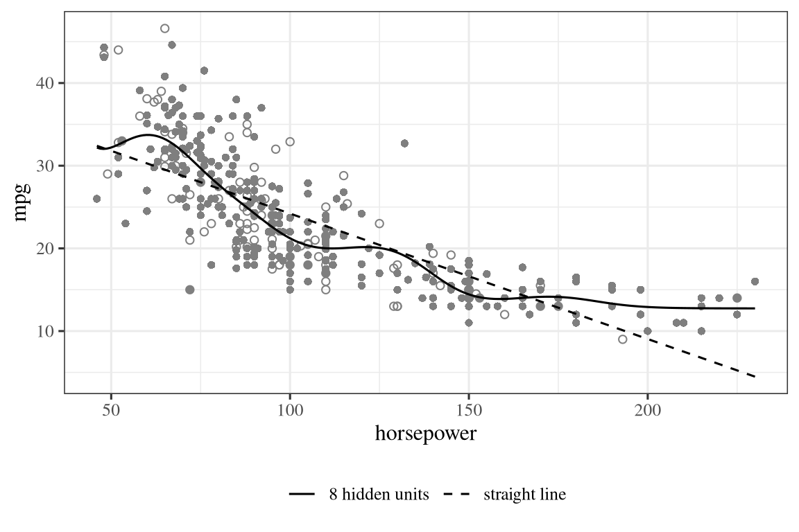
Exercise 47 (Watch the hidden width change a fit to real cars (part 4))
Exercise 47 (Watch the hidden width change a fit to real cars (part 4)) Use the setup of Exercise 44.
Say what the hidden units let the fit do that the line cannot.
Solution 47. Each hidden unit is a smooth step at its own centre, so a weighted sum of them can bend the curve. Fuel economy falls steeply at low horsepower and levels off at high horsepower, a bend that a line cannot follow.
Exercise 48 (Watch the hidden width change a fit to real cars (part 5))
Exercise 48 (Watch the hidden width change a fit to real cars (part 5)) Use the setup of Exercise 44.
The notes ask what \(L\) decides. Use your table to say what you would choose for \(L\) here, and why the training error alone could not tell you.
Solution 48. Choose the smallest \(L\) whose test error is close to the best in the table, because beyond that point extra units add parameters without improving the fit to new cars. The training error cannot make this choice: it measures how well the fit matches the rows it was fitted to, and a more flexible network can match those rows ever more closely whether or not it predicts new cars better. Only error on held-out rows can show where adding units stops helping.
Definition 1 (Autoencoder)
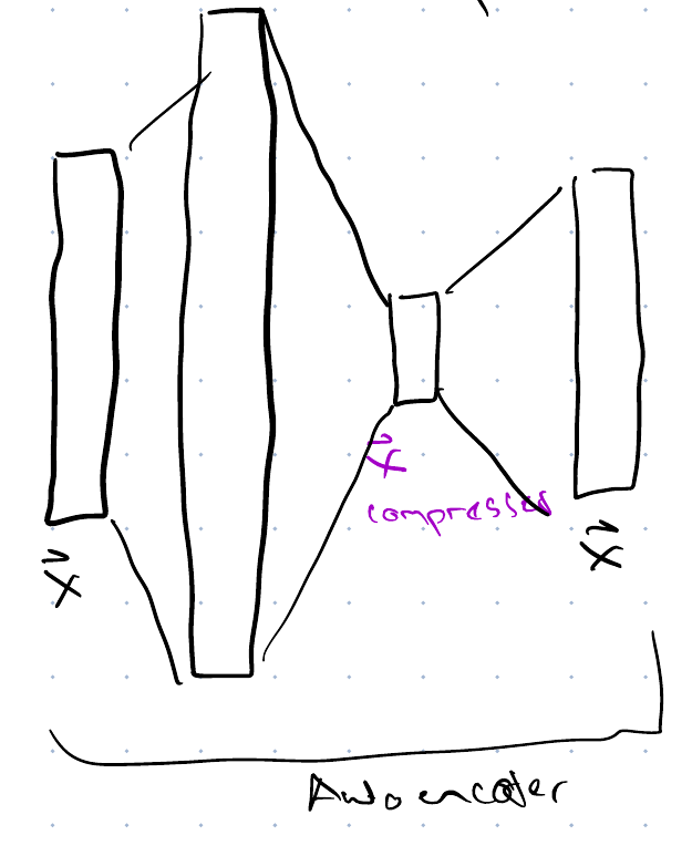
Definition 1 (Autoencoder) An autoencoder is a network trained to reproduce its own input [6]: its target is \(\vx\) itself, and a bottleneck layer in the middle (Exercise 42) holds a compressed representation of \(\vx\) from which the layers after the bottleneck layer rebuild \(\vx\).
Example 5 (Compressing six car measurements into two numbers)
Example 5 (Compressing six car measurements into two numbers) Take the \(6\) numeric features of the Auto data [5] that describe a car’s engine and body: cylinders, displacement, horsepower, weight, acceleration and year, standardized to mean \(0\) and variance \(1\). Train an autoencoder with a bottleneck of \(2\) units, so the network is \(6 \to 2 \to 6\) and its target is its own input. A network that ignored its input and always predicted the mean would have sMSE \(1\) on each standardized feature:
import numpy as np
import pandas as pd
from sklearn.neural_network import MLPRegressor

cols_ae = ["cylinders", "displacement", "horsepower", "weight", "acceleration", "year"]
auto_ae = pd.read_csv("data/auto.csv").dropna(subset=cols_ae)
X_ae = auto_ae[cols_ae].to_numpy(float)
X_ae = (X_ae - X_ae.mean(axis=0)) / X_ae.std(axis=0)

# The target is the input itself; the single hidden layer of 2 units is the bottleneck.
ae_fit = MLPRegressor(hidden_layer_sizes=(2,), activation="tanh", max_iter=5000,
                      random_state=0).fit(X_ae, X_ae)
mse_ae = np.mean((ae_fit.predict(X_ae) - X_ae) ** 2)
print(round(mse_ae, 3))0.198cols_ae <- c("cylinders", "displacement", "horsepower", "weight", "acceleration", "year")
auto_ae <- na.omit(read.csv("data/auto.csv")[, cols_ae])
X_ae <- scale(auto_ae)
# The target is the input itself; the single hidden layer of 2 units is the bottleneck.
set.seed(0)
ae_fit_r <- nnet::nnet(X_ae, X_ae, size = 2, linout = TRUE, maxit = 2000, trace = FALSE)
mse_ae_r <- mean((predict(ae_fit_r, X_ae) - X_ae)^2)
round(mse_ae_r, 3)[1] 0.15The autoencoder rebuilds the six features from two numbers with an sMSE of 0.15 in R (0.20 in Python), against \(1\) for the constant prediction. Both errors are measured on the cars the autoencoder was trained on, and from one random start, so they have no confidence interval: the fit chose its weights to make them small, and they say nothing about how well it would rebuild new cars. It can do this because the features are strongly related: heavy cars have more cylinders, bigger engines and more horsepower, so two numbers carry most of what the six do. The two hidden-unit values for a car are its compressed representation.
Read
GeeksforGeeks explains autoencoders [7].
Watch
- Hastie and Tibshirani introduce neural networks [8], video 10.1.
- Starmer gives the essential main ideas of neural networks [9].
Watch
- The CS229 lecture introduces neural networks [10], Lecture 10.
- Abu-Mostafa also gives a lecture on neural networks [11], Lecture 10.
Watch
Hutchinson covers:
- layers (4 min) [2]
- feed-forward networks and hidden layers (25 min) [2]
Read
GeeksforGeeks explains:
Read
The University of Washington’s CSE 446 slides cover neural nets [14], Lecture 19.
4 What a hidden unit can do
A hidden unit is \(\sigmoid(w_0 + \dprod{\vw}{\vx})\) — the same object logistic regression fits, now used as a feature rather than as a prediction. Asking what one of them can represent turns out to have a simple answer.
Exercise 49 (What a single unit computes)
Exercise 49 (What a single unit computes) Consider one hidden unit, \(\hidval = \sigmoid(\dprod{\vw}{\vx})\), with \(\vx \in \reals^{\ninputvars+1}\) carrying a constant \(1\).
Describe the set of \(\vx\) on which \(\hidval = \tfrac12\), and the sets on which \(\hidval > \tfrac12\) and \(\hidval < \tfrac12\).
Solution 49. \(\sigmoid(z) = \tfrac12\) exactly at \(z = 0\), and \(\sigmoid\) is strictly increasing, so
\[\hidval = \tfrac12 \iff \dprod{\vw}{\vx} = 0, \qquad \hidval > \tfrac12 \iff \dprod{\vw}{\vx} > 0, \qquad \hidval < \tfrac12 \iff \dprod{\vw}{\vx} < 0\]
The first is a hyperplane in \(\reals^{\ninputvars+1}\); in the original \(\ninputvars\) coordinates it is an affine hyperplane, positioned by the bias entry of \(\vw\). The other two are the open halfspaces on either side.
Exercise 50 (What a single unit computes (part 2))
Exercise 50 (What a single unit computes (part 2)) Use the setup of Exercise 49.
Replace \(\vw\) by \(t\vw\) and let \(t \to \infty\). What does \(\hidval\) converge to, at a point not on the set from Exercise 49? Conclude what a single unit computes in the limit, and name the object.
Solution 50. At a point with \(\dprod{\vw}{\vx} = z_0 \neq 0\), scaling gives \(\sigmoid(t z_0)\), and
\[\lim_{t\to\infty}\sigmoid(t z_0) = \begin{cases} 1 & z_0 > 0\\ 0 & z_0 < 0\end{cases}\]
since \(tz_0 \to \pm\infty\) with the sign of \(z_0\). So in the limit the unit computes the indicator of a halfspace: it returns \(1\) on one side of a hyperplane and \(0\) on the other. The direction of \(\vw\) fixes the orientation, the bias fixes the offset, and the magnitude fixes only how abruptly the unit switches — the same separation of direction from scale as in logistic regression.
Exercise 51 (What a single unit computes (part 3))
Exercise 51 (What a single unit computes (part 3)) Use the setup of Exercise 49.
The argument in Exercise 50 needs the qualification “not on the set from Exercise 49”. Say what happens there, and why no choice of \(t\) removes the qualification.
Solution 51. On the hyperplane itself \(z_0 = 0\), so
\[ \begin{aligned} \sigmoid(t \cdot 0) &= \sigmoid(0) \\ &= \tfrac12 \end{aligned} \]
for every \(t\). The limit is \(\tfrac12\) there, not \(0\) or \(1\).
No \(t\) removes this because the value at \(z_0 = 0\) does not depend on \(t\) at all. The convergence is pointwise off the hyperplane and never uniform near it: for any fixed \(t\) there are points either side within distance \(1/t\) of the boundary where the unit is still near \(\tfrac12\). That transition band is not a technicality to be dismissed: it makes the unit differentiable, and so makes gradient descent applicable at all. A true step function has zero derivative everywhere it is defined and would supply no gradient to train on.
Exercise 52 (What a single unit computes (part 4))
Exercise 52 (What a single unit computes (part 4)) Use the setup of Exercise 49.
Now restrict the inputs to \(\vx \in \{0,1\}^{\ninputvars}\). Exercise 50 says a unit computes a halfspace indicator; say what that becomes when only the corners of the cube are available, and how many distinct functions \(\{0,1\}^{\ninputvars} \to \{0,1\}\) there are in total. Exercise 53 asks which ones.
Solution 52. On the corners of the cube a halfspace indicator becomes a linearly separable Boolean function: those \(\{0,1\}^{\ninputvars} \to \{0,1\}\) functions whose \(1\)-corners can be cut off from the \(0\)-corners by a single hyperplane.
There are \(2^{2^{\ninputvars}}\) Boolean functions on \(\ninputvars\) inputs in total, since each of the \(2^{\ninputvars}\) corners may independently be sent to \(0\) or \(1\). At \(\ninputvars = 2\) that is \(16\), of which \(14\) are linearly separable — the two exceptions being XOR and its negation, which is Theorem 1 again in Boolean form. The count \(2^{2^{\ninputvars}}\) grows far faster than the number of halfspaces, so for larger \(\ninputvars\) almost no Boolean function is computable by one unit, so we need a hidden layer, as in Exercise 59.
When the inputs are binary, that halfspace becomes something familiar. Throughout what follows we use \(\sigmoid(10) \approx 1\) and \(\sigmoid(-10) \approx 0\).
Exercise 53 (Which gates can one unit compute?)
Exercise 53 (Which gates can one unit compute?) Take binary inputs \(x_1, x_2 \in \{0,1\}\) and one unit \(\hidval = \sigmoid(w_0 + w_1x_1 + w_2x_2)\). Read the output as the bit it is nearer to.
Write the pre-activation \(w_0 + w_1\predvar_1 + w_2\predvar_2\) on each of the four corners, in terms of the weights.
Solution 53. On the corners \((0,0)\), \((0,1)\), \((1,0)\) and \((1,1)\) the pre-activation is
\[w_0, \qquad w_0 + w_2, \qquad w_0 + w_1, \qquad w_0 + w_1 + w_2.\]
Exercise 54 (Which gates can one unit compute? (part 2))
Exercise 54 (Which gates can one unit compute? (part 2)) Use the setup of Exercise 53.
What does the unit have to arrange, corner by corner, to output a value near \(1\) on some corners and a value near \(0\) on the rest?
Solution 54. The unit outputs a value near \(1\) where the pre-activation is large and positive, and a value near \(0\) where it is large and negative. So the design problem is entirely about signs and margins: the pre-activation has to be positive, by a wide margin, on the corners that should give \(1\), and negative, by a wide margin, on the rest.
Exercise 55 (Which gates can one unit compute? (part 3))
Exercise 55 (Which gates can one unit compute? (part 3)) Use the setup of Exercise 53.
Which of NOT \(\predvar_1\), AND, OR and XOR can one unit compute?
Solution 55. The unit is on exactly where \(w_0 + w_1x_1 + w_2x_2 > 0\), which is one side of a line in the plane (Solution 50). So it can compute a Boolean function precisely when a line cuts that function’s \(1\)-corners off from its \(0\)-corners: the linearly separable functions, \(14\) of the \(16\) (Solution 52).
NOT \(x_1\), AND and OR are all among them. NOT \(x_1\) is on the edge \(x_1 = 0\), AND on the single corner \((1,1)\), and OR on every corner except \((0,0)\); in each case a line cuts those corners off from the others. Once a line does, the margins of Solution 54 follow directly: every corner sits a positive distance from the line, so multiplying all three weights by a large enough positive number pushes every pre-activation as far from zero as we like without moving the line.
Exercise 56 (Which gates can one unit compute? (part 4))
Exercise 56 (Which gates can one unit compute? (part 4)) Use the setup of Exercise 53.
Give a geometric reason for any of them that one unit cannot compute.
Solution 56. XOR is not. Its \(1\)-corners are \((0,1)\) and \((1,0)\). If both were strictly on the positive side of a line, so would be their midpoint \((\tfrac12, \tfrac12)\), since a half-plane is convex. But that is also the midpoint of \((0,0)\) and \((1,1)\), so at least one of those would be on the positive side too. This is Theorem 1 again, in Boolean form.
Exercise 57 (Which gates can one unit compute? (part 5))
Exercise 57 (Which gates can one unit compute? (part 5)) Use the setup of Exercise 53.
Evaluate \(\sigmoid(10)\) and \(\sigmoid(-10)\) to six decimal places. The output is never exactly \(0\) or \(1\): say why that is unavoidable for any finite weights, and why it is a feature rather than a defect.
Solution 57. \(\sigmoid(10) = 0.999955\) and \(\sigmoid(-10) = 0.000045\).
Exactness is impossible because \(\sigmoid(z) = 1/(1+e^{-z})\) and \(e^{-z} > 0\) for every finite \(z\), so \(\sigmoid(z) \in (0,1)\) strictly: the values \(0\) and \(1\) are approached and never attained. Larger weights move closer without reaching it, which is the separation problem seen from the other side.
It is a feature because it makes the unit differentiable. A true step function has derivative \(0\) wherever it is defined and no derivative at the jump, so gradient descent would receive no signal anywhere. The sigmoid trades exactness for a usable gradient, and Solution 51 shows what that trade gives up.
Exercise 58 (Which gates can one unit compute? (part 6))
Exercise 58 (Which gates can one unit compute? (part 6)) Use the setup of Exercise 53.
Take any corner \(c\) of the cube \(\{0,1\}^{\ninputvars}\). Show that some single unit is on at \(c\) and off at every other corner. An argument that such weights exist is enough; you do not need to write them down. You will use this in Exercise 68.
Solution 58. Every corner of the cube is a vertex of it: no corner is an average of the others. So \(c\) lies outside the convex hull of the remaining \(2^{\ninputvars} - 1\) corners, and a point outside a closed convex set can be strictly separated from it by a hyperplane. Put \(c\) on the positive side, and scale the weights up as in Solution 54 until every pre-activation is decisive.
One unit per corner, firing on that corner alone: this is the building block Exercise 68 counts.
Watch
- Sanderson introduces neurons and layers, from 2:42 [15, Ch. 1].
- He explains why networks have layers, from 5:31.
- He then compares ReLU with the sigmoid, from 17:03.
- Starmer shows ReLU in action [16].
5 What a layer of them can do
Exercise 1 said a linear boundary cannot represent XOR. Exercise 53 showed which pieces one unit can supply.
Exercise 59 (Two layers are enough for XOR)
Exercise 59 (Two layers are enough for XOR) Exercise 1 showed that no single linear boundary separates XOR. Exercise 53 showed that one unit can compute OR, and AND. Put the two facts together.
Write XOR as a Boolean expression in OR and AND. There is more than one right answer; pick one that uses each of OR and AND exactly once.
Solution 59. \(x_1 \text{ XOR } x_2 = (x_1 \text{ OR } x_2) \text{ AND NOT } (x_1 \text{ AND } x_2)\): at least one of them is on, and not both.
Exercise 60 (Two layers are enough for XOR (part 2))
Exercise 60 (Two layers are enough for XOR (part 2)) Use the setup of Exercise 59.
Design a network with two hidden units \(\hidvalof{1}, \hidvalof{2}\) and one output \(\outvar\) that computes your expression.
Solution 60. Take \(\hidvalof{1}\) to be an OR unit and \(\hidvalof{2}\) an AND unit, both reading \(x_1, x_2\). The output has to compute \(\hidvalof{1} \text{ AND NOT } \hidvalof{2}\).
Exercise 61 (Two layers are enough for XOR (part 3))
Exercise 61 (Two layers are enough for XOR (part 3)) Use the setup of Exercise 59.
Say which Boolean function each of the three units computes.
Solution 61. One hidden unit computes OR, the other computes AND, and the output computes \(\hidvalof{1} \text{ AND NOT } \hidvalof{2}\).
Exercise 62 (Two layers are enough for XOR (part 4))
Exercise 62 (Two layers are enough for XOR (part 4)) Use the setup of Exercise 59.
Use Exercise 55 to check that one unit can compute it.
Solution 62. Read as a function of \((\hidvalof{1}, \hidvalof{2})\), \(\hidvalof{1} \text{ AND NOT } \hidvalof{2}\) is on at the single corner \((1, 0)\). A line cuts one corner of the square off from the other three, so by Exercise 55 one more unit of the same kind computes it.
Exercise 63 (Two layers are enough for XOR (part 5))
Exercise 63 (Two layers are enough for XOR (part 5)) Use the setup of Exercise 59.
Tabulate \(\hidvalof{1}\), \(\hidvalof{2}\) and \(\outvar\) on all four corners, reading each unit as the bit it is nearer to, and check the output is right on each.
Solution 63. Reading each unit as its nearest bit:
| \(x_1\) | \(x_2\) | \(\hidvalof{1}\) | \(\hidvalof{2}\) | \(y\) | XOR |
|---|---|---|---|---|---|
| \(0\) | \(0\) | \(0\) | \(0\) | \(0\) | \(0\) |
| \(0\) | \(1\) | \(1\) | \(0\) | \(1\) | \(1\) |
| \(1\) | \(0\) | \(1\) | \(0\) | \(1\) | \(1\) |
| \(1\) | \(1\) | \(1\) | \(1\) | \(0\) | \(0\) |
Right on all four corners. The hidden values are only approximately \(0\) and \(1\), but we set the output unit’s margin in the same way as the hidden units’, so an error of order \(\sigmoid(-10)\) in its inputs moves its pre-activation by far less than that margin.
Exercise 64 (Two layers are enough for XOR (part 6))
Exercise 64 (Two layers are enough for XOR (part 6)) Use the setup of Exercise 59.
The hidden layer takes the four corners of the input square to four points in the \((\hidvalof{1}, \hidvalof{2})\) plane. Plot those four points, approximately.
Solution 64. The four corners land at approximately
\[(0,0) \mapsto (0,0), \quad (0,1) \mapsto (1,0), \quad (1,0) \mapsto (1,0), \quad (1,1) \mapsto (1,1).\]
Exercise 65 (Two layers are enough for XOR (part 7))
Exercise 65 (Two layers are enough for XOR (part 7)) Use the setup of Exercise 59.
Why is the output unit’s job now easy, when Exercise 1 said it was impossible?
Solution 65. The two corners that should give \(1\) have been mapped to the same point, \((1,0)\), and the two that should give \(0\) sit at \((0,0)\) and \((1,1)\). In the \((\hidvalof{1},\hidvalof{2})\) plane the problem is no longer XOR at all: the positive class is one point, and a line through it separates it from the other two. The line \(\hidvalof{1} - \hidvalof{2} = \tfrac{1}{2}\) will do.
So the output unit is not doing anything clever. It is solving a linearly separable problem, because the hidden layer handed it one. That is the whole idea: a network does not evade Exercise 1, it moves the data until the last layer’s linear boundary is enough.
Exercise 66 (Two layers are enough for XOR (part 8))
Exercise 66 (Two layers are enough for XOR (part 8)) Use the setup of Exercise 59.
In Exercise 1 you separated XOR by adding the feature \(\predvar_3 = \predvar_1\predvar_2\) by hand. Which of \(\hidvalof{1}, \hidvalof{2}\) is playing that role here?
Solution 66. \(\hidvalof{2}\) is the AND unit, and \(\predvar_1 \text{ AND } \predvar_2 = \predvar_1\predvar_2\) on \(\{0,1\}\), so \(\hidvalof{2}\) is the hand-built feature \(\predvar_3 = \predvar_1\predvar_2\) of Exercise 1, rediscovered.
Exercise 67 (Two layers are enough for XOR (part 9))
Exercise 67 (Two layers are enough for XOR (part 9)) Use the setup of Exercise 59.
State the difference between the two solutions in one sentence.
Solution 67. The difference is who chose it. In Exercise 1 you looked at the data, saw that a product would do it, and wrote the product down; here the same feature is a unit whose weights are numbers the fitting procedure could have found on its own.
That is the trade Exercise 8 set up. A basis expansion writes down every product up to some degree, and pays \(\binom{\ninputvars+L}{L}\) for the ones it does not need. A hidden layer writes down \(L\) features and lets the fit decide what they are, paying \(L(\ninputvars+1)\) parameters regardless of what it discovers.
Read
GeeksforGeeks explains how neural networks solve the XOR problem [17].
XOR took two hidden units. The natural next question is how many units an arbitrary function needs.
Exercise 68 (How many hidden units does a logic function need?)
Exercise 68 (How many hidden units does a logic function need?) XOR needed two hidden units. Ask what an arbitrary Boolean function \(f : \{0,1\}^{\ninputvars} \to \{0,1\}\) needs.
Exercise 58 showed that one unit can fire on one named corner of \(\{0,1\}^{\ninputvars}\) and nowhere else. Use that to write any \(f\) as a one-hidden-layer network. How many hidden units does your construction use, in terms of the number \(M\) of corners where \(f = 1\)?
Solution 68. Every corner where \(f = 1\) gets its own unit. Write \(M = |\{x : f(x) = 1\}|\) and list those corners \(c^{(1)}, \ldots, c^{(M)}\). For each corner \(c\), Solution 58 gives a unit \(\hidvalof{c}\) that outputs about \(1\) at \(x = c\) and about \(0\) everywhere else. So the construction uses \(M\) hidden units.
This is the disjunctive normal form (DNF) of \(f\) — \(f\) is true exactly when the input is one of the corners where it is true — written as a network.
Exercise 69 (How many hidden units does a logic function need? (part 2))
Exercise 69 (How many hidden units does a logic function need? (part 2)) Use the setup of Exercise 68.
Say what the output unit has to compute, and why the construction needs no more than an OR at the top.
Solution 69. At most one hidden unit is on at a time, because the corners are distinct and each unit fires on only its own. So the output has to answer “is any of them on”, which is an OR over \(M\) inputs. That OR, read as a function of the hidden layer, is off at the single corner where every \(\hidval\) is \(0\) and on everywhere else. A hyperplane cuts that one corner off, so one unit computes the OR (Exercise 55, in \(M\) dimensions). Nothing more elaborate is needed at the top, because the hidden layer has already done the work of recognizing each corner.
Exercise 70 (How many hidden units does a logic function need? (part 3))
Exercise 70 (How many hidden units does a logic function need? (part 3)) Use the setup of Exercise 68.
Bound \(M\) above. Then improve the bound by noticing that a network computing \(f\) is easily turned into one computing \(1 - f\).
Solution 70. \(M \leq 2^{\ninputvars}\), since there are only that many corners, so the construction never needs more than \(2^{\ninputvars}\) hidden units.
The bound halves. If \(f\) is \(1\) on more than half the corners, build a network for \(1 - f\) instead, which is \(1\) on fewer than half, and then negate the output unit’s weights and bias, which turns “is any of them on” into “are all of them off”. So \(\min(M, 2^{\ninputvars} - M) \leq 2^{\ninputvars-1}\) units always suffice.
Exercise 71 (How many hidden units does a logic function need? (part 4))
Exercise 71 (How many hidden units does a logic function need? (part 4)) Use the setup of Exercise 68.
The “off” hidden units do not output exactly \(0\), and there are up to \(2^{\ninputvars-1}\) of them, so we might expect their leakage into the output sum to grow with \(\ninputvars\) and eventually exceed the output’s margin. Suppose each corner unit’s pre-activation is \(m > 0\) at its own corner and falls by at least \(a > m\) for every coordinate in which the input disagrees with that corner. Bound the total leakage, by asking which off units contribute much, and show it grows only linearly in \(\ninputvars\).
Solution 71. Because the off units are not all equally off. Take an input \(\predvar\) and a corner unit whose corner differs from \(\predvar\) in \(k\) coordinates. Its pre-activation is at most \(m - ak\), so its output is at most \(\sigmoid(m - ak) < e^{m - ak}\), which falls exponentially in \(k\). There are \(\binom{\ninputvars}{k}\) corners at distance \(k\) from \(x\), so the total leakage from all the off units is at most
\[\sumto{k}{\ninputvars} \binom{\ninputvars}{k} e^{m - ak} = e^{m}\sb{\paren{1 + e^{-a}}^{\ninputvars} - 1} \approx \ninputvars\, e^{m - a} \quad\text{when } \ninputvars e^{-a} \ll 1.\]
The leakage is dominated by the at most \(\ninputvars\) units at distance \(1\), and grows only linearly in \(\ninputvars\), regardless of how large \(M\) is. The far-away units contribute nothing that matters, because \(\sigmoid\) falls exponentially in the distance faster than the number of corners at that distance grows.
Exercise 72 (How many hidden units does a logic function need? (part 5))
Exercise 72 (How many hidden units does a logic function need? (part 5)) Use the setup of Exercise 68.
Now take the specific function \(f(x) = x_1 \oplus x_2 \oplus \cdots \oplus x_{\ninputvars}\), the parity of the input. Exercise 70 gives a bound of order \(2^{\ninputvars}\) for it. Show that \(\ninputvars\) hidden units are in fact enough, by building the network from the quantities \(\mathbb{1}\{s \geq k\}\) where \(s = \sum_d \predvar_d\).
Solution 72. Let \(s = \sum_d \predvar_d\), the number of ones in the input, which runs \(0, 1, \ldots, \ninputvars\). Parity is the parity of \(s\). Write \(\mathbb{1}\{s \geq k\}\) for the indicator that at least \(k\) inputs are on, and check the alternating sum
\[ \begin{aligned} \sumto{k}{\ninputvars} (-1)^{k+1}\,\mathbb{1}\{s \geq k\} &= \underbrace{1 - 1 + 1 - \cdots}_{s \text{ terms}} \\ &= \begin{cases} 1 & s \text{ odd} \\ 0 & s \text{ even.}\end{cases} \end{aligned} \]
Exactly \(s\) of the indicators are on, so the sum telescopes to \(s \bmod 2\).
Each indicator is one hidden unit. The count \(s\) is a linear function of the input, so the corners with \(s \geq k\) and those with \(s \leq k - 1\) lie on opposite sides of the hyperplane \(s = k - \tfrac{1}{2}\), and a unit whose boundary is that hyperplane, with its weights scaled up, computes the indicator (Exercise 55, in \(\ninputvars\) dimensions). The output unit then needs to be on when the alternating sum of the \(\hidvalof{k}\) is \(1\) and off when it is \(0\). That sum is a linear function of the hidden layer, so a threshold on it at \(\tfrac{1}{2}\) is again one unit. So parity takes \(\ninputvars\) hidden units, not \(2^{\ninputvars-1}\).
Exercise 73 (How many hidden units does a logic function need? (part 6))
Exercise 73 (How many hidden units does a logic function need? (part 6)) Use the setup of Exercise 68.
Parity has half its corners set to \(1\), so Exercise 70’s bound is as bad for it as for any function, and yet Exercise 72 does it in \(\ninputvars\) units. What, then, does the \(O(2^{\ninputvars})\) figure actually describe?
Solution 73. The \(O(2^{\ninputvars})\) is the cost of the construction in parts 1–3, not a floor for any particular function. It says: here is a recipe that works for every \(f\), and here is its cost. It does not say that some named \(f\) forces you to pay it, and Solution 72 shows that the obvious candidate does not.
Parity looks like it should be the hard case. Parity is the standard example of a function that circuits of AND and OR gates cannot compute at constant depth without exponentially many gates. But a hidden unit is not an AND or an OR gate. It thresholds a weighted sum, so it can count, and counting is precisely what parity needs: the units \(\hidvalof{k}\) in Solution 72 are doing arithmetic on \(s\), which no fixed-depth collection of AND and OR gates can do. The DNF construction of Solution 68 discards that ability, using each unit as a single-corner detector when it could have been a counter.
Exercise 74 (How many hidden units does a logic function need? (part 7))
Exercise 74 (How many hidden units does a logic function need? (part 7)) Use the setup of Exercise 68.
Does anything survive as a statement about most functions?
Solution 74. Something does survive, but only on average. There are \(2^{2^{\ninputvars}}\) Boolean functions on \(\ninputvars\) bits (Exercise 49), a doubly exponential count, while a network with \(L\) hidden units is fixed by \((\ninputvars+1)L + (L+1)\) numbers. Suppose we store each number in \(b\) bits. Then there are at most \(2^{b((\ninputvars+1)L + L + 1)}\) networks, hence at most that many functions realisable with \(L\) units, and covering all \(2^{2^{\ninputvars}}\) functions needs
\[b\paren{(\ninputvars+1)L + L + 1} \geq 2^{\ninputvars}, \qquad\text{so}\qquad L \gtrsim \frac{2^{\ninputvars}}{b\ninputvars}.\]
All but a vanishing fraction of Boolean functions therefore need on the order of \(2^{\ninputvars} / \ninputvars\) hidden units. Replacing the \(b\)-bit fiction with a bound on how many distinct functions a real-parameter family can realise — a Vapnik–Chervonenkis (VC) dimension argument — changes the polynomial factors in \(\ninputvars\) and not the shape.
That argument counts, so it proves that almost every \(f\) is expensive without naming a single one, and it cannot name one: any \(f\) you can write down briefly is, by that very fact, drawn from a tiny and unrepresentative part of the \(2^{2^{\ninputvars}}\). Parity is an example. This is the representational question only. We take up next whether we can find such a network, given data rather than the function itself.
Watch
Starmer builds a network with several inputs and outputs [18].
6 Universal approximation
Introductions to networks usually state a strong guarantee. The guarantee is true, and we need to read it carefully.
Exercise 75 (What “universal approximator” promises, and what it does not)
Exercise 75 (What “universal approximator” promises, and what it does not) Introductions to neural networks often claim that they are universal approximators: any function can be approximated arbitrarily well by a network with enough hidden units. The claim is true. This exercise is about reading it carefully.
Take \(\ninputvars = 1\) and one hidden layer. Using two units, build a function that is about \(1\) on an interval \((a,b)\) and about \(0\) outside it.
Solution 75. Take the difference of two sigmoids with the same steepness and different offsets:
\[\text{bump}_{a,b}(x) = \sigmoidf{t(x-a)} - \sigmoidf{t(x-b)}, \qquad a < b.\] Each sigmoid is one hidden unit and the subtraction is two output weights, \(+1\) and \(-1\), so the bump costs two units. Larger \(t\) makes the two edges sharper.
Exercise 76 (What “universal approximator” promises, and what it does not (part 2))
Exercise 76 (What “universal approximator” promises, and what it does not (part 2)) Use the setup of Exercise 75.
Sketch the two sigmoids and their difference.
Solution 76. The first sigmoid switches on near \(a\) and the second near \(b\). For \(x \ll a\) both terms are near \(0\), so the difference is near \(0\). For \(x \gg b\) both are near \(1\), so the difference is near \(0\) again. Between \(a\) and \(b\) the first has switched on and the second has not, so the difference is near \(1\).
Exercise 77 (What “universal approximator” promises, and what it does not (part 3))
Exercise 77 (What “universal approximator” promises, and what it does not (part 3)) Use the setup of Exercise 75.
Use \(N\) of these bumps, side by side, to approximate a continuous \(f : [0,1] \to \reals\). How many hidden units does that cost?
Solution 77. Cut \([0,1]\) into \(N\) intervals of length \(1/N\) and put a bump on each. Each bump takes two hidden units, so this costs \(2N\) hidden units.
Exercise 78 (What “universal approximator” promises, and what it does not (part 4))
Exercise 78 (What “universal approximator” promises, and what it does not (part 4)) Use the setup of Exercise 75.
How should you choose each bump’s height?
Solution 78. Give bump \(j\) the output weight \(f\paren{(j + \tfrac{1}{2})/N}\), the value of \(f\) at the middle of that interval:
\[g(x) = \sum_{j=0}^{N-1} f\paren{\frac{j + \frac{1}{2}}{N}} \text{bump}_{j/N,\,(j+1)/N}(x).\]
Exercise 79 (What “universal approximator” promises, and what it does not (part 5))
Exercise 79 (What “universal approximator” promises, and what it does not (part 5)) Use the setup of Exercise 75.
Roughly how does the error behave as \(N\) grows, and why?
Solution 79. Since at most one bump is on at a time, \(g\) is a piecewise-constant approximation of \(f\) — a staircase — so the error on an interval is how far \(f\) moves across a length of \(1/N\). For differentiable \(f\) that is about \(\max|f'| / (2N)\): halving the interval width halves the error, so the error falls like \(1/N\), which is first order and not fast.
Measured on \(f(x) = \sin(2\pi x) + 0.3x^2\) over \([0.05, 0.95]\), with \(t = 25N\):
| \(N\) | hidden units | \(\max\abs{ g - f}\) |
|---|---|---|
| \(4\) | \(8\) | \(0.436\) |
| \(8\) | \(16\) | \(0.252\) |
| \(16\) | \(32\) | \(0.139\) |
| \(32\) | \(64\) | \(0.068\) |
| \(64\) | \(128\) | \(0.034\) |
| \(128\) | \(256\) | \(0.017\) |
Each doubling of \(N\) halves the error, as expected. Getting two decimal places took \(256\) hidden units for one input variable.
Exercise 80 (What “universal approximator” promises, and what it does not (part 6))
Exercise 80 (What “universal approximator” promises, and what it does not (part 6)) Use the setup of Exercise 75.
Now take \(\ninputvars = 2\) and try to build an indicator of the box \((a_1,b_1) \times (a_2,b_2)\). Show that you can do it with \(2\ninputvars\) units in a first hidden layer and one unit in a second. Then say what goes wrong if you try to assemble the same box out of one hidden layer in the obvious way.
Solution 80. Build the \(\ninputvars\) one-dimensional bumps in the first layer, at \(2\ninputvars\) units, then ask the second layer whether all \(\ninputvars\) of them are on:
\[\text{box}(x) = \sigmoidf{T\sb{\sumto{d}{\ninputvars} \text{bump}_{a_d,b_d}(x_d) - \paren{\ninputvars - \tfrac{1}{2}}}}.\]
Inside the box every bump is on and the sum is about \(\ninputvars\); outside, at least one is off and the sum is at most about \(\ninputvars-1\). Thresholding at \(\ninputvars - \tfrac{1}{2}\) separates the two. This is an AND over \(\ninputvars\) coordinates, and the second layer computes it.
Checked at \(\ninputvars = 2\) with \((a,b) = (0.3,0.6) \times (0.4,0.7)\), \(t = 300\), \(T = 40\): the box returns \(1.000000\) at interior points including the corners \((0.31,0.41)\) and \((0.59,0.69)\), and \(0.000000\) at \((0.45,0.2)\), \((0.1,0.55)\), \((0.1,0.1)\) and \((0.61,0.55)\).
In one hidden layer the obvious attempt fails. A single layer can only form \(\sum_m u_m\,\sigmoid(w_m^Tx + w_{0m})\), a weighted sum of halfspace-like ridges, and the AND you need is a threshold of a sum, not a sum. Adding the \(\ninputvars\) bumps without thresholding gives a function that is \(\ninputvars\) inside the box but also \(\ninputvars-1\) on the whole slab where all but one coordinate is in range — a plus-sign shape, not a box. Applying a threshold to the sum removes the slab, and the threshold is a second layer.
Exercise 81 (What “universal approximator” promises, and what it does not (part 7))
Exercise 81 (What “universal approximator” promises, and what it does not (part 7)) Use the setup of Exercise 75.
Continuing Exercise 76’s strategy into \(\ninputvars\) dimensions requires tiling the cube \([0,1]^{\ninputvars}\) with boxes. How many boxes, if each side is cut into \(N\) pieces?
Solution 81. Cutting each of \(\ninputvars\) sides into \(N\) pieces gives \(N^{\ninputvars}\) boxes, so the tiling costs \(N^{\ninputvars}\) second-layer units, exponential in \(\ninputvars\).
Exercise 82 (What “universal approximator” promises, and what it does not (part 8))
Exercise 82 (What “universal approximator” promises, and what it does not (part 8)) Use the setup of Exercise 75.
Compare that count with Exercise 8, and say which of the two is worse.
Solution 82. That is worse than Exercise 8. A basis expansion of degree \(L\) costs \(\binom{\ninputvars+L}{L} \approx \ninputvars^L/L!\), which is exponential in the degree \(L\) and only polynomial in the dimension \(\ninputvars\). The tiling is exponential in \(\ninputvars\) itself, and \(\ninputvars\) is the thing you do not get to choose. At \(\ninputvars = 784\), a modest degree-\(2\) expansion is \(308{,}505\) terms while a tiling at \(N = 2\) is \(2^{784}\) boxes.
Exercise 83 (What “universal approximator” promises, and what it does not (part 9))
Exercise 83 (What “universal approximator” promises, and what it does not (part 9)) Use the setup of Exercise 75.
The theorem holds for one hidden layer in any \(\ninputvars\), even though Exercise 77 says the tiling argument does not give it to you. What does that tell you about the kind of statement the theorem is?
Solution 83. That it is an existence theorem, proved by an argument that does not build the network. The tiling is one route to universality; it happens to need two layers and exponentially many units, and the theorem says neither of those is necessary for the conclusion. What it does not say is how few units are necessary — an existence proof that does not construct the object does not come with a count.
So “enough hidden units” in the statement carries real content, and the theorem leaves it unquantified. Exercise 68 is the same gap in the Boolean case: a construction gives \(2^{\ninputvars-1}\), a counting argument gives \(2^{\ninputvars}/\ninputvars\) for almost every function, and neither tells you what any particular function costs.
Exercise 84 (What “universal approximator” promises, and what it does not (part 10))
Exercise 84 (What “universal approximator” promises, and what it does not (part 10)) Use the setup of Exercise 75.
The Weierstrass approximation theorem says that polynomials are also universal approximators on a closed bounded interval. Given that, what does universality actually tell you about the choice between a network and a basis expansion?
Solution 84. That universality is not the distinguishing property. Both families are universal, so a claim that a network can approximate anything is not an argument for a network over a basis expansion; it rules out neither and recommends neither.
Cost and adaptivity differ. Exercise 8 fixes the features in advance and pays \(\binom{\ninputvars+L}{L}\) of them, most of which the data never needed. A hidden layer fixes the number of features at \(L\) and pays \(L(\ninputvars+1)\) parameters to let the fit choose what they are (Exercise 66). The question worth asking about an architecture is how many parameters it needs for the accuracy you want on the problem you have, and universality does not address it.
Exercise 85 (What “universal approximator” promises, and what it does not (part 11))
Exercise 85 (What “universal approximator” promises, and what it does not (part 11)) Use the setup of Exercise 75.
List what the theorem does not say. Consider at least: the number of units required; whether fitting finds the approximating network; and what happens when you have \(\nobs\) data points rather than the function itself.
Solution 85. The theorem is silent on all three.
How many units. No bound, as Solution 79 says. The honest reading of “any function can be well approximated by some network” is that no function is ruled out, not that any particular one is cheap.
Whether fitting finds it. The theorem is about representation: some setting of the weights approximates \(f\). Gradient descent searches a non-convex surface and is not promised to reach it — and the constructions here are a warning, since they use weights like \(t = 300\) that a fit starting from small random values and descending a gradient has no particular reason to visit. Representable and findable are different properties.
What happens with data. The theorem approximates a known \(f\) on a compact set. In practice you hold \(\nobs\) pairs \((\predvar_i, \outvar_i)\) and not \(f\), and a network with enough units to approximate any \(f\) has enough units to interpolate any \(\nobs\) points, noise included. Universality is therefore a statement about the prediction function family being large, which is exactly the condition under which fitting the training data says least about new data.
A fourth omission worth naming: the approximation holds on a compact set, fixed before the units are chosen. It promises nothing about \(x\) outside the region the argument was run on, which is the formal version of the usual warning not to extrapolate.
Watch
Weinberger discusses universal approximation, from 27:05 [19], Lecture 35.
Watch
Hutchinson covers the representational power of networks (23 min) [2].
Read
GeeksforGeeks explains the universal approximation theorem [20].
7 Depth and width
Exercise 75 part 3 already needed a second hidden layer to build a box. Nothing forces a network to stop at two. A deep network stacks several hidden layers, each taking the previous layer’s output as its input, and the back-propagation chapter writes out the forward rule for \(K\) of them. Two words describe the result, and they mean different quantities.
Definition 2 (Depth)
Definition 2 (Depth) The depth of a network is its number of layers of weights: \(K + 1\) for a network with \(K\) hidden layers, counted as in the counting-layers note of Section 3. A network is deep when it has more than one hidden layer.
Definition 3 (Width)
Definition 3 (Width) The width of a layer is its number of units. The hidden layer of Equation 1 has width \(L\).
Example 6 (Two networks for fuel economy with the same number of parameters)
Example 6 (Two networks for fuel economy with the same number of parameters) Predict mpg in the Auto data [5] from the \(6\) other numeric columns: cylinders, displacement, horsepower, weight, acceleration and year. Compare a network with two hidden layers, of widths \(8\) and \(4\), with a network with one hidden layer. List each network’s layer sizes, read off its depth and widths, and count its weights and biases:
# Layer sizes from the input to the output: 6 inputs, hidden layers, 1 output.
deep_dw = [6, 8, 4, 1]
wide_dw = [6, 12, 1]

def n_params_dw(sizes):
    """Each layer has a weight matrix (units x inputs) and one bias per unit."""
    return sum(n_out * n_in + n_out for n_in, n_out in zip(sizes[:-1], sizes[1:]))

for name, sizes in [("deep", deep_dw), ("wide", wide_dw)]:
    # K hidden layers means K + 1 layers of weights, which is the depth.
    print(name, "depth", len(sizes) - 1, "widths", sizes[1:-1], "parameters", n_params_dw(sizes))
deep depth 3 widths [8, 4] parameters 97
wide depth 2 widths [12] parameters 97# Layer sizes from the input to the output: 6 inputs, hidden layers, 1 output.
deep_dw <- c(6, 8, 4, 1)
wide_dw <- c(6, 12, 1)
# Each layer has a weight matrix (units x inputs) and one bias per unit.
n_params_dw <- function(sizes) {
n_in <- head(sizes, -1)
n_out <- tail(sizes, -1)
sum(n_out * n_in + n_out)
}
# K hidden layers means K + 1 layers of weights, which is the depth.
data.frame(
network = c("deep", "wide"),
depth = c(length(deep_dw) - 1, length(wide_dw) - 1),
parameters = c(n_params_dw(deep_dw), n_params_dw(wide_dw))
)The first network has \(K = 2\) hidden layers, so its depth is \(3\), and its hidden layers have widths \(8\) and \(4\). The second has \(K = 1\), depth \(2\), and one hidden layer of width \(12\). Both have 97 parameters, so the choice between them is not about size: we can spend the same budget on depth or on width. Only the first is deep in the sense of the definition, because it has more than one hidden layer.
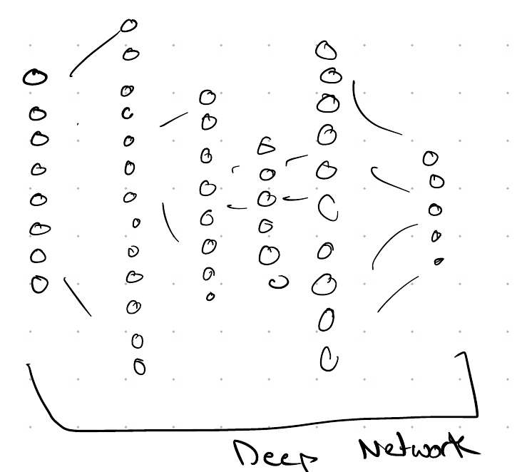
Depth and width are independent settings, and the rest of this section is about why they are not interchangeable.
Nothing requires the hidden layers to match each other, and in principle every weight matrix could have its own shape and every layer its own non-linearity. In practice:
We usually give the hidden layers all the same width, so we describe the architecture by two numbers, the depth and the common width, rather than by one width per hidden layer.
We usually use the same \(f\) in every hidden layer.
The task fixes the output layer’s width: \(C\) units, one per class, or one unit for scalar regression.
The task fixes the output activation \(g\) as well, exactly as it was for one hidden layer in Exercise 22 part 4.
So the free choices in an ordinary feedforward architecture are the depth, the common width, and the hidden non-linearity. All three are hyperparameters: nothing in the data determines them, and we choose them by the procedure of model selection like any other.
If depth only had to compete with width on what is representable, it would not be worth using: Exercise 75 says one hidden layer already approximates any continuous function. The argument for depth is about efficiency of representation rather than about what is representable at all.
The simplest version of it counts regions. A network whose non-linearity is piecewise linear — the rectified linear unit \(f(a) = \max(0, a)\), say — computes a piecewise linear function, and the number of linear pieces it can divide the input space into is a reasonable measure of how complex a decision boundary it can draw. The largest number of pieces a network can produce grows exponentially in the depth and only polynomially in the width [21]. A deep network can therefore match a shallow one’s expressiveness with far fewer parameters, and the gap widens as the functions get more complex.
Networks also differ in how their units are connected, not only in how many there are.
Definition 4 (Fully connected layer)
Definition 4 (Fully connected layer) A layer is fully connected when every one of its units reads every unit of the layer below it [22]. Every layer in this chapter is fully connected.
Example 7 (Every unit reads every input)
Example 7 (Every unit reads every input) A fully connected layer of \(L = 4\) units on the \(\ninputvars = 6\) numeric features of the Auto data [5] has a weight matrix \(W\) with \(L\) rows and \(\ninputvars\) columns. Row \(k\) holds the weights of unit \(k\), one for every input. Build such a layer with random weights, apply it to the first car, and check that changing any one input changes every unit’s output:
import numpy as np
import pandas as pd

cols_fc = ["cylinders", "displacement", "horsepower", "weight", "acceleration", "year"]
auto_fc = pd.read_csv("data/auto.csv").dropna(subset=cols_fc)
x_fc = auto_fc[cols_fc].iloc[0].to_numpy(float)
x_fc = (x_fc - auto_fc[cols_fc].mean().to_numpy()) / auto_fc[cols_fc].std().to_numpy()

rng_fc = np.random.default_rng(0)
W_fc = rng_fc.normal(size=(4, 6))     # one row per unit, one column per input
b_fc = np.zeros(4)
out_fc = np.tanh(W_fc @ x_fc + b_fc)

# Nudge each input in turn: how many of the 4 outputs move?
moved_fc = []
for j in range(6):
    x_nudged = x_fc.copy()
    x_nudged[j] += 0.1
    moved_fc.append(int(np.sum(np.tanh(W_fc @ x_nudged + b_fc) != out_fc)))
print(W_fc.shape, W_fc.size, moved_fc)
(4, 6) 24 [4, 4, 4, 4, 4, 4]cols_fc <- c("cylinders", "displacement", "horsepower", "weight", "acceleration", "year")
auto_fc <- na.omit(read.csv("data/auto.csv")[, cols_fc])
x_fc <- as.numeric(scale(auto_fc)[1, ])
set.seed(0)
W_fc <- matrix(rnorm(4 * 6), nrow = 4, ncol = 6) # one row per unit, one column per input
b_fc <- rep(0, 4)
out_fc <- tanh(W_fc %*% x_fc + b_fc)
# Nudge each input in turn: how many of the 4 outputs move?
moved_fc <- sapply(1:6, function(j) {
x_nudged <- x_fc
x_nudged[j] <- x_nudged[j] + 0.1
sum(tanh(W_fc %*% x_nudged + b_fc) != out_fc)
})
list(shape = dim(W_fc), n_weights = length(W_fc), outputs_moved = moved_fc)$shape
[1] 4 6
$n_weights
[1] 24
$outputs_moved
[1] 4 4 4 4 4 4The layer has \(4 \times 6 =\) 24 weights, one for every pair of an input and a unit. Each nudge moves all 4 of the layer’s outputs, because every unit reads every input. A layer that connected each unit to only a few neighbouring inputs, as convolutional layers do, would have zeros in most of \(W\), and a nudge would reach only the units that read that input.
Full connection is one choice among several, and each choice encodes an assumption about the data. A convolutional layer has each unit read only a small neighbourhood and share its weights across positions, which assumes that what counts as a useful local pattern does not depend on where it occurs. A recurrent layer feeds a unit’s own output back as an input at the next step, which assumes the inputs form a sequence whose earlier terms matter. And a deeper stack of narrow layers and a shallower stack of wide ones can hold the same number of weights and still learn quite different functions. Convolutional and Recurrent Networks builds the first two kinds of layer.
Watch
Weinberger compares wide and deep networks, from 38:20 [19], Lecture 35.
Watch
Hutchinson covers deep networks (21 min) [2].
Watch
Starmer explains:
8 Choosing an objective
Everything so far has been about what a network can represent. Fitting one needs a loss, and the loss is not a free choice: it is a statement about the distribution of \(y\) given \(x\), whether or not you state it.
Exercise 86 (Choosing the loss, and why it is not a free choice)
Exercise 86 (Choosing the loss, and why it is not a free choice) Exercise 22 left the output activation \(g\) to be chosen by the task. We have to choose the loss too, and the two choices are not independent.
For regression the usual loss is squared error, and for classification it is cross-entropy:
\[\lossf{\outvar, \eoutvar} = \paren{\outvar - \eoutvar}^2, \qquad \lossf{\vy, \modmemf{x}} = -\sumto{c}{C} y_c \log \modmemof{c}\paren{x},\]
where \(\eoutvar = \modmemf{\predvar}\) is the fitted value.
Neither is an arbitrary choice. For squared error, name a distribution for \(\outvar\) given \(\predvar\) whose log-likelihood is the negative of that loss, up to a constant and a positive factor, and carry out the derivation. Linear regression states this one without deriving it; the point here is to say what it assumes.
Solution 86. Squared error is the Gaussian assumption. Take \(y \mid x \sim \mathcal{N}\paren{\modmemf{x}, \varpar}\) with \(\varpar\) fixed. Over independent training points the log-likelihood is
\[\llik = \sumin \sb{-\tfrac{1}{2}\log(2\pi\varpar) - \frac{\paren{\outvar_i - \eoutvar_i}^2}{2\varpar}},\]
where \(\eoutvar_i = \modmemf{\predvar_i}\) is the fitted value. The only parameter-dependent part is \(-\frac{1}{2\varpar}\sumin \paren{\outvar_i - \eoutvar_i}^2\). Maximizing \(\llik\) is minimizing the sum of squared errors.
Exercise 87 (Choosing the loss, and why it is not a free choice (part 2))
Exercise 87 (Choosing the loss, and why it is not a free choice (part 2)) Use the setup of Exercise 86.
For cross-entropy, name a distribution for \(\outvar\) given \(\predvar\) whose log-likelihood is the negative of that loss, up to a constant and a positive factor, and carry out the derivation. Logistic regression derives this one; the point here is to say what it assumes.
Solution 87. Cross-entropy is the categorical assumption. Take \(\vy\) one-hot and model \(P(y_c = 1 \mid x) = \modmemof{c}\paren{x}\), so that \(P(\vy \mid x) = \prod_c \modmemof{c}\paren{x}^{y_c}\). Then
\[\llik = \sumin \sumto{c}{C} y_{ic} \log \modmemof{c}\paren{x_i},\]
the negative of the summed cross-entropy.
So the two losses are the same procedure — maximum likelihood — under two different assumptions about what kind of thing \(y\) is. Writing down a loss is writing down a noise model, whether or not you state it. The Gaussian assumption also makes squared error a poor fit for classification before any gradient argument: a label in \(\{0,1\}\) is not a continuous quantity with symmetric additive noise, and the model is wrong about the response in an obvious way.
Exercise 88 (Choosing the loss, and why it is not a free choice (part 3))
Exercise 88 (Choosing the loss, and why it is not a free choice (part 3)) Use the setup of Exercise 86.
Nothing stops you writing squared error for a classification problem. Take one binary output \(\modmem = \sigmoid(z)\) and a label \(\outvar \in \{0,1\}\). Differentiate both losses with respect to the pre-activation \(z\).
Solution 88. With \(\modmem = \sigmoid(z)\):
\[\deriv{z}\paren{y - \sigmoid(z)}^2 = -2\paren{y - \sigmoid(z)}\,\sigmoid(z)\paren{1 - \sigmoid(z)},\]
using \(\sigmoid'(z) = \sigmoid(z)(1-\sigmoid(z))\), while for binary cross-entropy \(L = -\outvar\log\sigmoid(z) - (1-\outvar)\log(1-\sigmoid(z))\) the \(\sigmoid'\) cancels against the \(1/\sigmoid\) from the logarithm and leaves
\[\frac{\partial L}{\partial z} = \sigmoid(z) - y.\]
Exercise 89 (Choosing the loss, and why it is not a free choice (part 4))
Exercise 89 (Choosing the loss, and why it is not a free choice (part 4)) Use the setup of Exercise 86.
Evaluate both derivatives at \(\outvar = 1\) and \(z = -10\) — the model is confidently wrong.
Solution 89. At \(y = 1\) and \(z = -10\), the sigmoid gives \(\sigmoid(z) =\) 0.000045:
| loss | \(\partial L/\partial z\) |
|---|---|
| squared error | \(-0.000091\) |
| cross-entropy | \(-0.999955\) |
Exercise 90 (Choosing the loss, and why it is not a free choice (part 5))
Exercise 90 (Choosing the loss, and why it is not a free choice (part 5)) Use the setup of Exercise 86.
Solution 90. Cross-entropy still supplies a gradient of essentially full size, and squared error supplies almost none. The reason is the \(\sigmoid'(z)\) factor. Being confidently wrong makes \(\sigmoid(z)\) near \(0\), so \(\sigmoid'(z)\) is near \(0\) too, and squared error multiplies the error by it. Cross-entropy’s logarithm cancels that factor exactly, and this cancellation makes the pairing standard.
Exercise 91 (Choosing the loss, and why it is not a free choice (part 6))
Exercise 91 (Choosing the loss, and why it is not a free choice (part 6)) Use the setup of Exercise 86.
By what factor do they differ?
Solution 91. Squared error supplies a gradient about 11,000 times smaller than cross-entropy’s.
Exercise 92 (Choosing the loss, and why it is not a free choice (part 7))
Exercise 92 (Choosing the loss, and why it is not a free choice (part 7)) Use the setup of Exercise 86.
Plot, or tabulate, the squared-error derivative as \(z\) runs from \(-10\) to \(+5\).
Solution 92. Sweeping \(z\) at \(y = 1\):
| \(z\) | \(\sigmoid(z)\) | squared error | cross-entropy |
|---|---|---|---|
| \(-10\) | \(0.000045\) | \(-0.000091\) | \(-0.999955\) |
| \(-5\) | \(0.006693\) | \(-0.013207\) | \(-0.993307\) |
| \(-2\) | \(0.119203\) | \(-0.184956\) | \(-0.880797\) |
| \(0\) | \(0.500000\) | \(-0.250000\) | \(-0.500000\) |
| \(2\) | \(0.880797\) | \(-0.025031\) | \(-0.119203\) |
| \(5\) | \(0.993307\) | \(-0.000089\) | \(-0.006693\) |
Exercise 93 (Choosing the loss, and why it is not a free choice (part 8))
Exercise 93 (Choosing the loss, and why it is not a free choice (part 8)) Use the setup of Exercise 86.
Where is it largest?
Solution 93. The squared-error derivative is largest in magnitude at \(z = 0\), where the model is maximally uncertain, and approaches zero in both directions.
Exercise 94 (Choosing the loss, and why it is not a free choice (part 9))
Exercise 94 (Choosing the loss, and why it is not a free choice (part 9)) Use the setup of Exercise 86.
Say why that shape is the wrong one for learning.
Solution 94. So it pushes hardest on the points the model is least sure about, and barely at all on the points it has got badly wrong — the wrong way round. Cross-entropy’s derivative is monotone in \(z\): the more wrong the prediction, the larger the gradient, which is the shape you want.
Note that squared error’s derivative is also small at \(z = +5\), where the model is confidently right. That part is fine and both losses do it. The defect is specifically the left tail.
Exercise 95 (Choosing the loss, and why it is not a free choice (part 10))
Exercise 95 (Choosing the loss, and why it is not a free choice (part 10)) Use the setup of Exercise 86.
Now do Exercise 87 for the matched combinations: identity output with squared error, sigmoid output with binary cross-entropy, and softmax output with cross-entropy. Write \(\partial L / \partial z_c\) in each case.
Solution 95.
| output \(g\) | loss | \(\partial L / \partial z_c\) |
|---|---|---|
| identity | \(\tfrac{1}{2}(y - \modmem)^2\) | \(\modmem - y\) |
| sigmoid | binary cross-entropy | \(\sigmoid(z) - \outvar\) |
| softmax | cross-entropy | \(\modmemof{c} - y_c\) |
Exercise 96 (Choosing the loss, and why it is not a free choice (part 11))
Exercise 96 (Choosing the loss, and why it is not a free choice (part 11)) Use the setup of Exercise 86.
What do the three answers have in common?
Solution 96. All three matched combinations give the same thing.
In every case the derivative with respect to the output pre-activation is prediction minus target. We checked the softmax case numerically at \(\vz = (2, -1, 0.5)\) with the target in class \(2\): central differences give \((+0.785597, -0.960887, +0.175290)\), and \(\modmem - \vy\) gives the same three numbers.
Exercise 97 (Choosing the loss, and why it is not a free choice (part 12))
Exercise 97 (Choosing the loss, and why it is not a free choice (part 12)) Use the setup of Exercise 86.
What advantage does that give you when you implement backpropagation?
Solution 97. That is the benefit of the pairing. Backpropagation starts from \(\partial L/\partial z\) at the output and pushes it backward through the layers, so this is the quantity it needs first, and the matched pair makes it a subtraction rather than a product of an error with a derivative that may be near zero. The same cancellation explains Solution 88: the two facts are one fact.
Mismatching the pair — softmax with squared error, say — is not an error the code will catch. It runs, and it trains slowly for the reason Solution 89 gives.
Exercise 98 (Choosing the loss, and why it is not a free choice (part 13))
Exercise 98 (Choosing the loss, and why it is not a free choice (part 13)) Use the setup of Exercise 86.
A network with $g = $ softmax and cross-entropy loss, trained on data it fits perfectly, drives the loss toward \(0\). What happens to \(\norm{ U}\) meanwhile?
Solution 98. \(\norm{ U}\) grows without bound. Cross-entropy reaches \(0\) only in the limit \(\modmemof{c} \to 1\) on every training point, which needs the correct class’s pre-activation to exceed the others by an unbounded margin. The direction of \(U\) settles while its scale grows without bound.
Exercise 99 (Choosing the loss, and why it is not a free choice (part 14))
Exercise 99 (Choosing the loss, and why it is not a free choice (part 14)) Use the setup of Exercise 86.
Which earlier exercise is this?
Solution 99. This is the separation problem, since Exercise 29 showed the output layer is multinomial logistic regression with \(B = U\). The remedy carries over unchanged: penalize \(\norm{ U}^2\), or stop early. A network adds a second place for it to happen. \(W\) is fit by the same descent on the same objective, so nothing stops its scale from growing without bound too, and Exercise 40’s observation that a hidden layer is never inert has a downside here as well.
Watch
Starmer explains cross-entropy [25] as a network’s loss.
Read
GeeksforGeeks explains loss functions in deep learning [26].
9 Regularizing a network
Exercise 100 (A network that fits the training set too well)
Exercise 100 (A network that fits the training set too well) A fully connected network reaches near-zero training loss, but its validation loss is much higher and rises as training continues. List the ways covered in these notes to reduce the gap without changing the data collected, and say what each one does to the fit.
Solution 100. A network has so many parameters that it can fit noise, so each remedy limits how closely it can. The notes develop five, in four different places:
Weight decay shrinks the weights at every step, which is an \(\lpnorm{2}\) penalty under plain gradient descent. See Weight decay.
Early stopping halts training when the validation loss stops improving, so the parameters have less time to move away from their initial values. See Regularizing without a penalty.
Data augmentation trains on label-preserving transformations of the examples, which tells the network what it should ignore. See Regularizing without a penalty.
Dropout zeroes random units during training, so no unit can rely on a particular other unit, and approximates averaging an ensemble of subnetworks. See Ensembling neural networks.
Smaller networks: fewer units or layers limit what the network can represent. See Depth and width.
The strength of each is a hyperparameter, so we tune each on the validation set, as in Model Selection.
10 Where this goes next
Two topics remain.
Fitting. We find \(W\) and \(U\) by gradient descent, as in the gradient descent chapter, with one complication: a network is a composition, so the derivative with respect to \(W\) has to pass back through \(f\). Doing that efficiently is back-propagation, the subject of the next chapter.
Watch
- Hastie and Tibshirani explain how neural networks are fitted [8], video 10.6.
- Their Python lab fits a multilayer network to handwritten digits.
Depth. Section 7 gave the case for depth in representation. Depth is cheap to write — the next chapter shows the gradient recursion is the same at every layer — but costly to train. Gradient Descent covers much of what makes deep networks train well.
11 Further reading
Goodfellow et al. [27], Chapter 6
James et al. [5], Chapter 10
Hastie et al. [28], Chapter 11
Starmer [29], on neural networks, and Starmer [30], which builds from a single network up to transformers, with PyTorch tutorials
References
[1]
Wikipedia contributors, “Perceptron — Wikipedia, the free encyclopedia.” 2026. Available: https://en.wikipedia.org/wiki/Perceptron
[2]
B. Hutchinson, “DATA 471/571 (machine learning) and CSCI 481/581 (deep learning) video lectures.” Western Washington University. Accessed: Sep. 28, 2026. [Online]. Available: https://facultyweb.cs.wwu.edu/~hutchib2/video_lectures/data371/
[3]
GeeksforGeeks, “What is perceptron.” GeeksforGeeks, tutorial article, 2026. Available: https://www.geeksforgeeks.org/deep-learning/what-is-perceptron-the-simplest-artificial-neural-network/
[4]
GeeksforGeeks, “Activation functions in neural networks.” GeeksforGeeks, tutorial article, 2026. Available: https://www.geeksforgeeks.org/machine-learning/activation-functions-neural-networks/
[5]
G. James, D. Witten, T. Hastie, and R. Tibshirani, An introduction to statistical learning with applications in R, 2nd ed. Springer, 2021. Available: https://www.statlearning.com/
[6]
Wikipedia contributors, “Autoencoder — Wikipedia, the free encyclopedia.” 2026. Available: https://en.wikipedia.org/wiki/Autoencoder
[7]
GeeksforGeeks, “Autoencoders in machine learning.” GeeksforGeeks, tutorial article, 2026. Available: https://www.geeksforgeeks.org/machine-learning/auto-encoders/
[8]
T. Hastie, R. Tibshirani, and J. Taylor, “Statistical learning with python.” Stanford Online, lecture videos on YouTube, 2023. Available: https://www.youtube.com/playlist?list=PLoROMvodv4rPP6braWoRt5UCXYZ71GZIQ
[9]
J. Starmer, “The essential main ideas of neural networks.” StatQuest, video on YouTube, 2020. Available: https://www.youtube.com/watch?v=CqOfi41LfDw
[10]
A. Ng et al., “CS229: Machine learning, autumn 2018.” Stanford Online, lecture videos on YouTube, 2018. Available: https://www.youtube.com/playlist?list=PLoROMvodv4rMiGQp3WXShtMGgzqpfVfbU
[11]
Y. S. Abu-Mostafa, “Learning from data: CS 156 lectures.” Caltech, lecture videos on YouTube, 2012. Available: https://www.youtube.com/playlist?list=PLD63A284B7615313A
[12]
GeeksforGeeks, “Introduction to neural networks.” GeeksforGeeks, tutorial article, 2026. Available: https://www.geeksforgeeks.org/deep-learning/neural-networks-a-beginners-guide/
[13]
GeeksforGeeks, “Feedforward neural network.” GeeksforGeeks, tutorial article, 2026. Available: https://www.geeksforgeeks.org/deep-learning/feedforward-neural-network/
[14]
N. Jaques, “CSE 446/546: Machine learning, lecture slides.” University of Washington, 2026. Accessed: Oct. 12, 2026. [Online]. Available: https://courses.cs.washington.edu/courses/cse446/26sp/schedule/lectures/
[15]
G. Sanderson, “Neural networks.” 3Blue1Brown, video series on YouTube; chapters 5 and 6 added in 2024, 2017. Available: https://www.youtube.com/playlist?list=PLZHQObOWTQDNU6R1_67000Dx_ZCJB-3pi
[16]
J. Starmer, “Neural networks pt. 3: ReLU in action.” StatQuest, video on YouTube, 2020. Available: https://www.youtube.com/watch?v=68BZ5f7P94E
[17]
GeeksforGeeks, “How neural networks solve the XOR problem.” GeeksforGeeks, tutorial article, 2025. Available: https://www.geeksforgeeks.org/artificial-intelligence/how-neural-networks-solve-the-xor-problem/
[18]
J. Starmer, “Neural networks pt. 4: Multiple inputs and outputs.” StatQuest, video on YouTube, 2021. Available: https://www.youtube.com/watch?v=83LYR-1IcjA
[19]
K. Weinberger, “CS4780: Machine learning for intelligent systems, spring 2017.” Cornell University, lecture videos on YouTube, 2017. Available: https://www.youtube.com/playlist?list=PLl8OlHZGYOQ7bkVbuRthEsaLr7bONzbXS
[20]
GeeksforGeeks, “Universal approximation theorem for neural networks.” GeeksforGeeks, tutorial article, 2025. Available: https://www.geeksforgeeks.org/deep-learning/universal-approximation-theorem-for-neural-networks/
[21]
G. Montúfar, R. Pascanu, K. Cho, and Y. Bengio, “On the number of linear regions of deep neural networks,” in Advances in neural information processing systems, 2014. Available: https://arxiv.org/abs/1402.1869
[22]
Wikipedia contributors, “Multilayer perceptron — Wikipedia, the free encyclopedia.” 2026. Available: https://en.wikipedia.org/wiki/Multilayer_perceptron
[23]
J. Starmer, “Neural networks part 8: Image classification with convolutional neural networks (CNNs).” StatQuest, video on YouTube, 2021. Available: https://www.youtube.com/watch?v=HGwBXDKFk9I
[24]
J. Starmer, “Recurrent neural networks (RNNs), clearly explained.” StatQuest, video on YouTube, 2022. Available: https://www.youtube.com/watch?v=AsNTP8Kwu80
[25]
J. Starmer, “Neural networks part 6: Cross entropy.” StatQuest, video on YouTube, 2021. Available: https://www.youtube.com/watch?v=6ArSys5qHAU
[26]
GeeksforGeeks, “Loss functions in deep learning.” GeeksforGeeks, tutorial article, 2026. Available: https://www.geeksforgeeks.org/deep-learning/loss-functions-in-deep-learning/
[27]
I. Goodfellow, Y. Bengio, and A. Courville, Deep learning. MIT Press, 2016. Available: https://www.deeplearningbook.org/
[28]
T. Hastie, R. Tibshirani, and J. Friedman, The elements of statistical learning: Data mining, inference, and prediction, 2nd ed. Springer, 2009. Available: https://hastie.su.domains/ElemStatLearn/
[29]
J. Starmer, The StatQuest illustrated guide to machine learning. StatQuest Publications, 2022. Available: https://statquest.org/statquest-store/
[30]
J. Starmer, The StatQuest illustrated guide to neural networks and AI: With hands-on examples in PyTorch. Independently published, 2025. Available: https://statquest.org/statquest-store/
[31]
Data Science Learning Community, “Introduction to statistical learning using R (islr06).” Book club meeting recordings on YouTube, 2023. Available: https://www.youtube.com/playlist?list=PL3x6DOfs2NGjlhpKMiWsDcKL2nngwXROq
[32]
Data Science Learning Community, “Introduction to statistical learning using Python (islp03).” Book club meeting recordings on YouTube, 2025. Available: https://www.youtube.com/playlist?list=PL3x6DOfs2NGgbSNh0UG87rrM-z5LiKLZp
[33]
A. Ng, “What is a neural network?” DeepLearning.AI, Deep Learning Specialization, Course 1; video on YouTube, 2017. Available: https://www.youtube.com/watch?v=n1l-9lIMW7E
[34]
A. Ng, “Neural network representations.” DeepLearning.AI, Deep Learning Specialization, Course 1; video on YouTube, 2017. Available: https://www.youtube.com/watch?v=CcRkHl75Z-Y
[35]
A. Ng, “Activation functions.” DeepLearning.AI, Deep Learning Specialization, Course 1; video on YouTube, 2017. Available: https://www.youtube.com/watch?v=Xvg00QnyaIY
[36]
A. Ng, “Why non-linear activation functions.” DeepLearning.AI, Deep Learning Specialization, Course 1; video on YouTube, 2017. Available: https://www.youtube.com/watch?v=NkOv_k7r6no
[37]
A. Ng, “Why deep representations?” DeepLearning.AI, Deep Learning Specialization, Course 1; video on YouTube, 2017. Available: https://www.youtube.com/watch?v=5dWp1mw_XNk