Fitting Logistic Regression

Last modified: 2026-11-19

Show code
# The Python chunks import these packages; reticulate provisions them.
library(reticulate) # nolint: undesirable_function_linter
py_packages <- c(
  "numpy", "pandas", "statsmodels", "scipy", "scikit-learn", "matplotlib",
  "plotly"
)
py_require(py_packages)

Source

This material was a section of the logistic regression page. It carries the same sources: Brian Hutchinson’s Fall 2025 lecture notes, Kameron Decker Harris’ 2022 weekly notes and Logan Sizemore’s Spring 2025 lectures, as described there.

1 Fitting the model by maximum likelihood

The form of the model is now fixed, and the parameter vector \(\vcoef\) remains to be estimated. Logistic regression is a probability model, so maximum likelihood gives a criterion for choosing \(\vcoef\): the value that makes the observed labels most probable.

Maximum likelihood also determines the loss function. Exercise 1, Exercise 2 and Exercise 3 derive that loss, Exercise 5 and Exercise 8 show why squared-error loss on the probabilities is unsuitable, and Exercise 7 graphs one observation’s contribution to the log-likelihood for each label.

Exercise 1 (Probability of a binary outcome in one formula)

Exercise 1 (Probability of a binary outcome in one formula) The log-odds exercise specified the model: \(\Pr[Y = 1 \mid \vx] = \sigmoidf{\dprod{\vcoef}{\vx}}\). It did not specify how to estimate \(\vcoef\). Let \(\prob_i = \sigmoidf{\dprod{\vcoef}{\vx_i}}\) be the probability that the model assigns to observation \(i\) having label \(1\).

Express \(\Pr[Y_i = y_i \mid \vx_i]\) as a single formula that holds for both \(y_i = 0\) and \(y_i = 1\), and check it at each value.

Solution 1. \[\Pr[Y_i = y_i \mid \vx_i] = \prob_i^{y_i}\paren{1 - \prob_i}^{1 - y_i}\]

At \(y_i = 1\), the second factor is \((1-\prob_i)^0 = 1\), so the expression equals \(\prob_i\). At \(y_i = 0\), the first factor is \(\prob_i^0 = 1\), so the expression equals \(1 - \prob_i\). Each value is the probability that the model gives to that outcome, so the single expression covers both cases.

Each exponent is either \(0\) or \(1\), so one factor equals \(1\), and the expression equals the factor for the observed outcome.

Lemma 1 (Probability mass of one Bernoulli outcome)

Lemma 1 (Probability mass of one Bernoulli outcome) If \(\Outvar_i \mid \vpredvar_i \sim \Bernoulli\paren{\prob_i}\) and \(\outvar_i \in \set{0, 1}\), then

\[\Prf{\Outvar_i = \outvar_i \given \vpredvar_i} = \prob_i^{\outvar_i}\paren{1 - \prob_i}^{1 - \outvar_i}.\]

Proof

Proof. By Solution 1.

Example 1 (The probability mass of one outcome)

Example 1 (The probability mass of one outcome) Let \(\prob_i = 0.8\). Lemma 1 gives the probabilities of the two outcomes, which equal the values from R’s dbinom and SciPy’s bernoulli.pmf:

p_bpmf <- 0.8
c(p_bpmf^1 * (1 - p_bpmf)^0, p_bpmf^0 * (1 - p_bpmf)^1)
[1] 0.8 0.2
dbinom(c(1, 0), size = 1, prob = p_bpmf)
[1] 0.8 0.2
from scipy.stats import bernoulli

p_bpmf = 0.8
print([p_bpmf**1 * (1 - p_bpmf)**0, p_bpmf**0 * (1 - p_bpmf)**1])
[0.8, 0.19999999999999996]
print(bernoulli.pmf([1, 0], p_bpmf))
[0.8 0.2]

Figure 1 plots the two values.

Show code
bpmf_outcomes <- c(0, 1)
bpmf_mass <- dbinom(bpmf_outcomes, size = 1, prob = 0.8)
bpmf_y <- factor(bpmf_outcomes)
bpmf_fig <- tibble::tibble(y = bpmf_y, mass = bpmf_mass)
bpmf_fills <- c("0" = "#0072B2", "1" = "#D55E00")
bpmf_limits <- c(0, 1)
bpmf_fig |>
  ggplot2::ggplot(ggplot2::aes(y, mass, fill = y)) +
  ggplot2::geom_col(width = 0.5) +
  ggplot2::geom_text(ggplot2::aes(label = mass), vjust = -0.4) +
  ggplot2::scale_fill_manual(values = bpmf_fills, guide = "none") +
  ggplot2::scale_y_continuous(limits = bpmf_limits) +
  ggplot2::labs(x = "Outcome", y = "Probability mass")
Show code
import matplotlib.pyplot as plt
from scipy.stats import bernoulli

fig, ax = plt.subplots(figsize=(4, 3), layout="constrained")
masses_bpmf = bernoulli.pmf([0, 1], 0.8)
bars_bpmf = ax.bar(["0", "1"], masses_bpmf, color=["#0072B2", "#D55E00"], width=0.5);
ax.bar_label(bars_bpmf, fmt="%.1f");
ax.set_ylim(0, 1);
ax.set_xlabel("Outcome");
ax.set_ylabel("Probability mass");
plt.show()
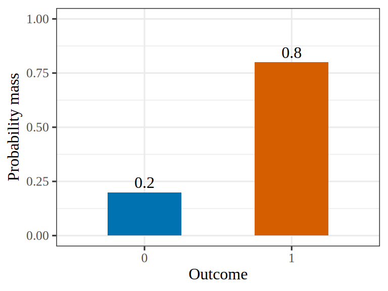
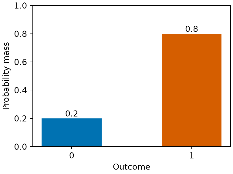
Figure 1: The probability masses of the two outcomes for \(\prob_i = 0.8\). The outcome \(1\) has probability \(0.8\) and the outcome \(0\) has probability \(0.2\).
(a)
Bar chart of the two probability masses for a probability of 0.8. A blue bar for the outcome 0 has height 0.2, and a vermilion bar for the outcome 1 has height 0.8, each labelled with its height.
(b)
Bar chart of the two probability masses for a probability of 0.8. A blue bar for the outcome 0 has height 0.2, and a vermilion bar for the outcome 1 has height 0.8, each labelled with its height.

Exercise 2 (Likelihood of the dataset)

Exercise 2 (Likelihood of the dataset) Using the single-observation probability from Exercise 1, express the likelihood \(L(\vcoef)\) of the full dataset in terms of the \(\prob_i = \sigmoidf{\dprod{\vcoef}{\vx_i}}\) and labels \(y_i\), and state the assumption required.

Solution 2. \[L(\vcoef) = \prodin \prob_i^{y_i}\paren{1 - \prob_i}^{1 - y_i}, \qquad \prob_i = \sigmoidf{\dprod{\vcoef}{\vx_i}}\]

The product form requires that the observations be conditionally independent given their features. Conditional independence is a different assumption from independence of the \(Y_i\) themselves, and neither assumption implies the other. Two patients with similar features have similar \(\prob_i\), so their outcomes can be correlated when the features are not held fixed, and the model allows that correlation. Conditional independence rules out datasets in which \(y_1\) carries information about \(y_2\) beyond what \(\vx_1\) and \(\vx_2\) provide. Two patients from the same household can share exposures that the features do not record, and repeated measurements on the same subject, or students within one classroom, are further examples. Such data violate conditional independence and need a method that accounts for the grouping, such as a model with a shared random effect, or standard errors that allow for correlation within groups.

Lemma 2 (Likelihood of conditionally independent Bernoulli outcomes)

Lemma 2 (Likelihood of conditionally independent Bernoulli outcomes) If \(\Outvar_1, \dots, \Outvar_n\) are conditionally independent given \(\vpredvar_1, \dots, \vpredvar_n\) with \(\Outvar_i \mid \vpredvar_i \sim \Bernoulli\paren{\prob_i}\), where \(\prob_i\) is determined by the coefficients \(\vcoef\) and the observed outcomes are \(\outvar_i \in \set{0, 1}\), the likelihood is

\[L(\vcoef) = \prodin \prob_i^{\outvar_i}\paren{1 - \prob_i}^{1 - \outvar_i}.\]

Proof

Proof. By Solution 2.

Example 2 (The likelihood of three outcomes)

Example 2 (The likelihood of three outcomes) Consider the outcomes \((1, 0, 1)\) with \((\prob_1, \prob_2, \prob_3) = (0.9, 0.2, 0.7)\). Lemma 2 gives the product of the three probability masses:

y_bl <- c(1, 0, 1)
p_bl <- c(0.9, 0.2, 0.7)
prod(p_bl^y_bl * (1 - p_bl)^(1 - y_bl))
[1] 0.504
import numpy as np

y_bl = np.array([1, 0, 1])
p_bl = np.array([0.9, 0.2, 0.7])
print(np.prod(p_bl**y_bl * (1 - p_bl)**(1 - y_bl)))
0.504

Figure 2 plots each factor and their product.

Show code
bl_names <- c("i = 1", "i = 2", "i = 3", "product")
bl_y <- c(1, 0, 1)
bl_p <- c(0.9, 0.2, 0.7)
bl_mass <- bl_p^bl_y * (1 - bl_p)^(1 - bl_y)
bl_product <- prod(bl_mass)
bl_values <- c(bl_mass, bl_product)
bl_shown <- round(bl_values, 3)
bl_what <- factor(bl_names, levels = bl_names)
bl_kinds <- c("observation", "observation", "observation", "product")
bl_fig <- tibble::tibble(what = bl_what, value = bl_values, kind = bl_kinds)
bl_fills <- c(observation = "#0072B2", product = "#D55E00")
bl_limits <- c(0, 1)
bl_fig |>
  ggplot2::ggplot(ggplot2::aes(what, value, fill = kind)) +
  ggplot2::geom_col(width = 0.6) +
  ggplot2::geom_text(ggplot2::aes(label = bl_shown), vjust = -0.4) +
  ggplot2::scale_fill_manual(values = bl_fills, guide = "none") +
  ggplot2::scale_y_continuous(limits = bl_limits) +
  ggplot2::labs(x = NULL, y = "Probability mass")
Show code
import matplotlib.pyplot as plt
import numpy as np

y_blf = np.array([1, 0, 1])
p_blf = np.array([0.9, 0.2, 0.7])
mass_blf = p_blf**y_blf * (1 - p_blf)**(1 - y_blf)
fig, ax = plt.subplots(figsize=(5, 3), layout="constrained")
bars_blf = ax.bar(["i = 1", "i = 2", "i = 3", "product"], [*mass_blf, np.prod(mass_blf)],
                  color=["#0072B2"] * 3 + ["#D55E00"], width=0.6);
ax.bar_label(bars_blf, fmt="%.3f");
ax.set_ylim(0, 1);
ax.set_ylabel("Probability mass");
plt.show()
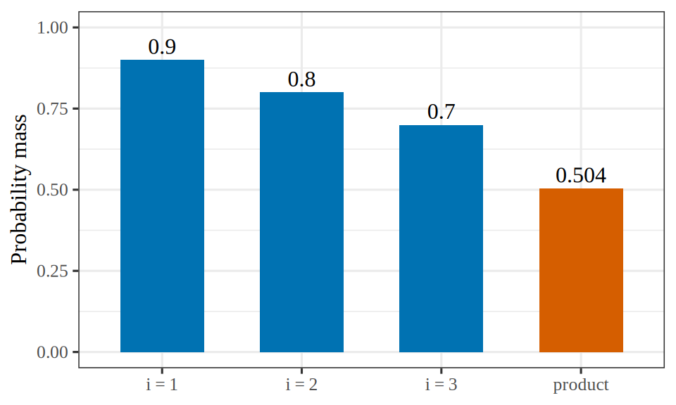
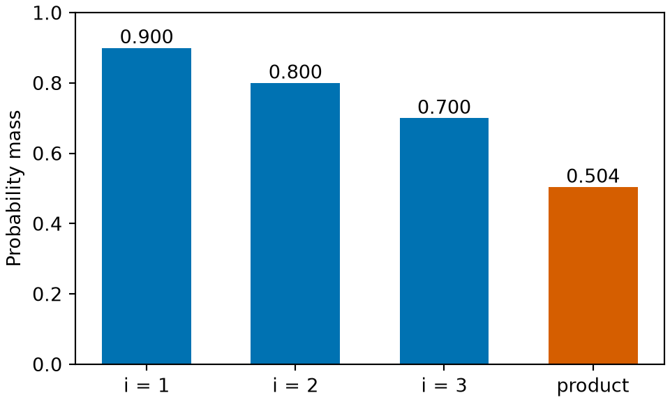
Figure 2: The probability mass of each observed outcome (blue) and the likelihood, their product (vermilion).
(a)
Bar chart of four values. Three blue bars, one for each observation, show the probability mass of its outcome: 0.9, 0.8 and 0.7. A vermilion bar labelled product shows their product, 0.504.
(b)
Bar chart of four values. Three blue bars, one for each observation, show the probability mass of its outcome: 0.9, 0.8 and 0.7. A vermilion bar labelled product shows their product, 0.504.

Exercise 3 (Log-likelihood of the dataset)

Exercise 3 (Log-likelihood of the dataset) Take the logarithm of the likelihood \(L(\vcoef)\) from Exercise 2 and simplify.

Solution 3. \[ \begin{aligned} \llik(\vcoef) &= \log L(\vcoef) && \text{(definition of log-likelihood)} \\ &= \log\paren{\prodin \prob_i^{y_i}\paren{1 - \prob_i}^{1 - y_i}} && \text{(likelihood of the dataset)} \\ &= \sumin \log\paren{\prob_i^{y_i}\paren{1 - \prob_i}^{1 - y_i}} && \text{(log of a product)} \\ &= \sumin\sb{\log\paren{\prob_i^{y_i}} + \log\paren{\paren{1 - \prob_i}^{1 - y_i}}} && \text{(log of a product)} \\ &= \sumin\sb{y_i \log \prob_i + (1-y_i)\log\paren{1 - \prob_i}} && \text{(log of a power)} \end{aligned} \]

The second line uses the likelihood from Solution 2.

Maximizing \(\llik(\vcoef)\) is equivalent to minimizing \(-\llik(\vcoef)\), which is the total log loss. Minimizing it adds no assumption to the maximum likelihood fit for conditionally independent Bernoulli outcomes.

Exercise 4 (Log-likelihood of the dataset (part 1b))

Exercise 4 (Log-likelihood of the dataset (part 1b)) Use the setup of Exercise 3.

Give two reasons to work with the log-likelihood \(\log L(\vcoef)\) rather than the likelihood \(L(\vcoef)\) of Exercise 2.

Solution 4. This continues Solution 3.

There are two reasons to work with \(\llik(\vcoef)\).

  1. Arithmetic. \(L(\vcoef)\) is a product of \(n\) numbers each below \(1\), so for \(n\) in the thousands it underflows to \(0\) in floating point, and every candidate \(\vcoef\) evaluates to \(0\). The logarithm turns the product into a sum of terms of moderate size.
  2. Optimization. \(\log\) is strictly increasing, so it does not change the maximizer, and a sum is differentiated term by term: the gradient of \(\llik(\vcoef)\) is the sum of \(n\) per-observation gradients. Stochastic gradient descent uses a few of its terms at each step.

Lemma 3 (Log-likelihood of conditionally independent Bernoulli outcomes)

Lemma 3 (Log-likelihood of conditionally independent Bernoulli outcomes) Under the assumptions of Lemma 2, the log-likelihood is

\[\llik(\vcoef) = \sumin\sb{\outvar_i \log \prob_i + (1-\outvar_i)\log\paren{1 - \prob_i}}.\]

Proof

Proof. By Solution 3.

Example 3 (The log-likelihood of three outcomes)

Example 3 (The log-likelihood of three outcomes) With the outcomes and probabilities of Example 2, Lemma 3 gives the log-likelihood as a sum, which equals the log of the likelihood:

y_bll <- c(1, 0, 1)
p_bll <- c(0.9, 0.2, 0.7)
sum(y_bll * log(p_bll) + (1 - y_bll) * log(1 - p_bll))
[1] -0.685179
log(prod(p_bll^y_bll * (1 - p_bll)^(1 - y_bll)))
[1] -0.685179
import numpy as np

y_bll = np.array([1, 0, 1])
p_bll = np.array([0.9, 0.2, 0.7])
print(np.sum(y_bll * np.log(p_bll) + (1 - y_bll) * np.log(1 - p_bll)))
-0.6851790109107685
print(np.log(np.prod(p_bll**y_bll * (1 - p_bll)**(1 - y_bll))))
-0.6851790109107684

Figure 3 plots each term and their sum.

Show code
bll_names <- c("i = 1", "i = 2", "i = 3", "sum")
bll_y <- c(1, 0, 1)
bll_p <- c(0.9, 0.2, 0.7)
bll_logmass <- bll_y * log(bll_p) + (1 - bll_y) * log(1 - bll_p)
bll_sum <- sum(bll_logmass)
bll_values <- c(bll_logmass, bll_sum)
bll_shown <- round(bll_values, 3)
bll_what <- factor(bll_names, levels = bll_names)
bll_kinds <- c("observation", "observation", "observation", "sum")
bll_fig <- tibble::tibble(what = bll_what, value = bll_values, kind = bll_kinds)
bll_fills <- c(observation = "#0072B2", sum = "#D55E00")
bll_limits <- c(-0.8, 0)
bll_fig |>
  ggplot2::ggplot(ggplot2::aes(what, value, fill = kind)) +
  ggplot2::geom_col(width = 0.6) +
  ggplot2::geom_text(ggplot2::aes(label = bll_shown), vjust = 1.4) +
  ggplot2::scale_fill_manual(values = bll_fills, guide = "none") +
  ggplot2::scale_y_continuous(limits = bll_limits) +
  ggplot2::labs(x = NULL, y = "Log of the probability mass")
Show code
import matplotlib.pyplot as plt
import numpy as np

y_bllf = np.array([1, 0, 1])
p_bllf = np.array([0.9, 0.2, 0.7])
logmass_bllf = y_bllf * np.log(p_bllf) + (1 - y_bllf) * np.log(1 - p_bllf)
fig, ax = plt.subplots(figsize=(5, 3), layout="constrained")
bars_bllf = ax.bar(["i = 1", "i = 2", "i = 3", "sum"], [*logmass_bllf, logmass_bllf.sum()],
                   color=["#0072B2"] * 3 + ["#D55E00"], width=0.6);
ax.bar_label(bars_bllf, fmt="%.3f", label_type="edge", padding=-14);
ax.set_ylim(-0.8, 0);
ax.set_ylabel("Log of the probability mass");
plt.show()
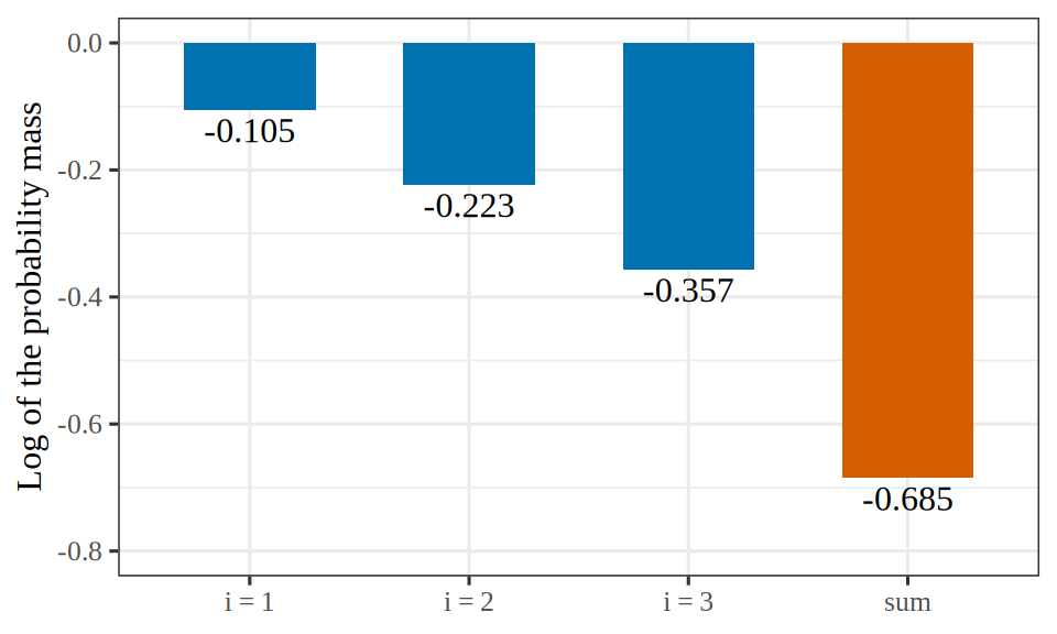
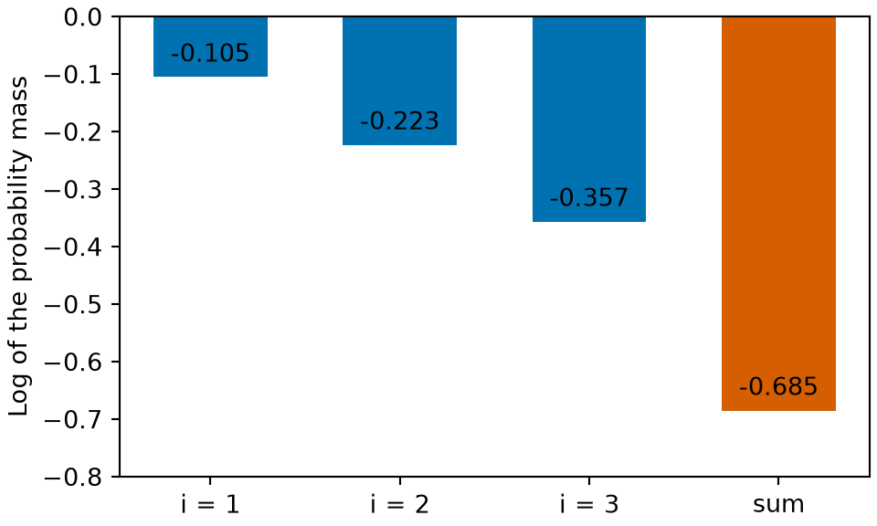
Figure 3: The log of each observation’s probability mass (blue) and the log-likelihood, their sum (vermilion).
(a)
Bar chart of four negative values. Three blue bars, one for each observation, show the log of its probability mass: -0.105, -0.223 and -0.357. A vermilion bar labelled sum shows their sum, -0.685.
(b)
Bar chart of four negative values. Three blue bars, one for each observation, show the log of its probability mass: -0.105, -0.223 and -0.357. A vermilion bar labelled sum shows their sum, -0.685.

Exercise 5 (Negative log-likelihood on a positive observation)

Exercise 5 (Negative log-likelihood on a positive observation) Consider one observation with label \(y_i = 1\) in the log-likelihood of Exercise 3. This exercise works with \(-\log L(\vcoef)\), the negative of the log-likelihood, because it treats that negative as a loss to compare with squared-error loss, and a loss is minimized rather than maximized. Give its contribution to \(-\log L(\vcoef)\) at \(\prob_i = 0.9\), \(0.5\), \(0.1\), and \(0.01\), to three significant figures.

Solution 5. With \(y_i = 1\), observation \(i\)’s contribution to \(-\log L(\vcoef)\) is \(-\log \prob_i\):

Show code
llp_prob <- c(0.9, 0.5, 0.1, 0.01)
knitr::kable(
  data.frame(
    prob = llp_prob,
    loss = formatC(-log(llp_prob), digits = 3, format = "fg", flag = "#")
  ),
  col.names = c("$\\prob_i$", "$-\\log \\prob_i$")
)
\(\prob_i\) \(-\log \prob_i\)
0.90 0.105
0.50 0.693
0.10 2.30
0.01 4.61

Exercise 6 (Negative log-likelihood on a positive observation (part 1b))

Exercise 6 (Negative log-likelihood on a positive observation (part 1b)) Use the setup of Exercise 5.

State what happens to the contribution of an observation with \(y_i = 1\) to \(-\log L\) as \(\prob_i \to 0\).

Solution 6. This continues Solution 5.

For an observation with \(y_i = 1\), the loss \(-\log \prob_i\) of Solution 5 increases without bound as \(\prob_i \to 0\). The model never gives \(\prob_i = 0\) exactly, because \(\prob_i = \sigmoidf{\dprod{\vcoef}{\vx_i}}\) is in \((0, 1)\), but no finite upper bound holds for the loss of an observation with \(y_i = 1\).

Exercise 7 (Graphing one observation’s log-likelihood contribution)

Exercise 7 (Graphing one observation’s log-likelihood contribution) In the log-likelihood of Lemma 3, observation \(i\) with label \(y_i\) contributes \(y_i \log \prob_i + (1 - y_i)\log\paren{1 - \prob_i}\). Graph this contribution against \(\prob_i\) over the interval \((0, 1)\), as one curve for \(y_i = 1\) and one for \(y_i = 0\).

Solution 7. For label \(y_i = 1\) the contribution is \(\log \prob_i\), and for \(y_i = 0\) it is \(\log\paren{1 - \prob_i}\). Figure 4 shows both curves.

  • \(y_i = 1\): the curve increases in \(\prob_i\), approaches \(0\) as \(\prob_i \to 1\), and tends to \(-\infty\) as \(\prob_i \to 0\).
  • \(y_i = 0\): the curve decreases in \(\prob_i\), approaches \(0\) as \(\prob_i \to 0\), and tends to \(-\infty\) as \(\prob_i \to 1\).

Each curve is the other reflected about \(\prob_i = 1/2\). Both curves are negative on all of \((0, 1)\), and each approaches \(0\) only as the probability that the model gives the observed label approaches \(1\).

Show code
lcc_prob <- seq(0.005, 0.995, length.out = 400)
lcc_loglik_pos <- log(lcc_prob)
lcc_prob_neg <- 1 - lcc_prob
lcc_loglik_neg <- log(lcc_prob_neg)
lcc_pos <- tibble::tibble(
  prob = lcc_prob,
  contribution = lcc_loglik_pos,
  label = "y = 1"
)
lcc_neg <- tibble::tibble(
  prob = lcc_prob,
  contribution = lcc_loglik_neg,
  label = "y = 0"
)
lcc_curves <- dplyr::bind_rows(lcc_pos, lcc_neg)
lcc_colours <- c("y = 1" = "#0072B2", "y = 0" = "#D55E00")
lcc_linetypes <- c("y = 1" = "solid", "y = 0" = "dashed")
lcc_curves |>
  ggplot2::ggplot() +
  ggplot2::aes(
    x = prob,
    y = contribution,
    colour = label,
    linetype = label
  ) +
  ggplot2::geom_line() +
  ggplot2::scale_colour_manual(values = lcc_colours) +
  ggplot2::scale_linetype_manual(values = lcc_linetypes) +
  ggplot2::labs(
    x = "Predicted probability of the label 1",
    y = "Log-likelihood contribution",
    colour = NULL,
    linetype = NULL
  )
Show code
import matplotlib.pyplot as plt
import numpy as np

lcc_prob = np.linspace(0.005, 0.995, 400)
fig, ax = plt.subplots(figsize=(5, 4), layout="constrained")
ax.plot(lcc_prob, np.log(lcc_prob), color="#0072B2", linestyle="-", label="y = 1");
ax.plot(lcc_prob, np.log(1 - lcc_prob), color="#D55E00", linestyle="--", label="y = 0");
ax.set_xlabel("Predicted probability of the label 1");
ax.set_ylabel("Log-likelihood contribution");
fig.legend(loc="outside lower center", ncol=2);
plt.show()
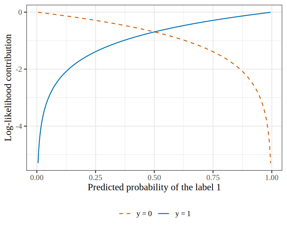
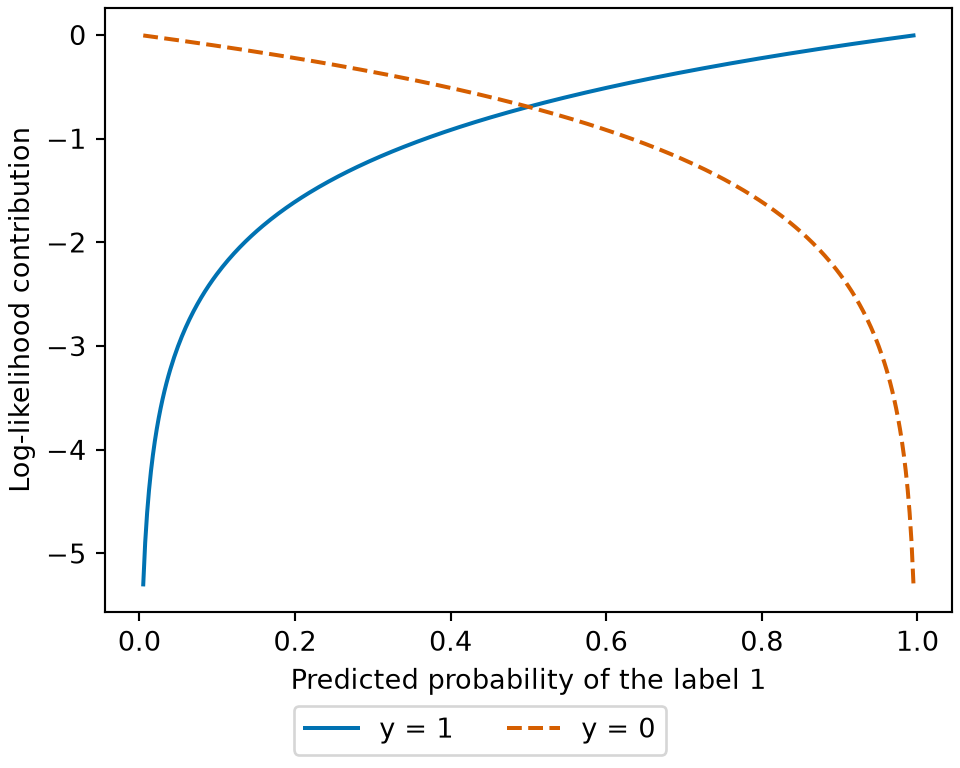
Figure 4: One observation’s contribution to the log-likelihood of Lemma 3, for each label, as the predicted probability \(\prob_i\) moves across \((0, 1)\). Each curve approaches \(0\) as the probability of the observed label approaches \(1\), and tends to \(-\infty\) as that probability approaches \(0\).
(a)
Line plot of one observation's log-likelihood contribution against the predicted probability from 0 to 1. The solid blue curve, for a label of 1, rises from about -5.3 at probability 0.005 toward 0 at probability 1. The dashed vermilion curve, for a label of 0, falls from about -0.005 at probability 0.005 to about -5.3 at probability 0.995. The two curves cross at probability 0.5, where both equal about -0.69.
(b)
Line plot of one observation's log-likelihood contribution against the predicted probability from 0 to 1. The solid blue curve, for a label of 1, rises from about -5.3 at probability 0.005 toward 0 at probability 1. The dashed vermilion curve, for a label of 0, falls from about -0.005 at probability 0.005 to about -5.3 at probability 0.995. The two curves cross at probability 0.5, where both equal about -0.69.

Exercise 8 (Why squared error on the probabilities is unsuitable)

Exercise 8 (Why squared error on the probabilities is unsuitable) Under squared-error loss, the positive observation of Exercise 5 contributes \((\prob_i - y_i)^2\), which never exceeds \(1\), however small \(\prob_i\) is. Explain what that upper bound allows a fitted model to do without incurring a large loss.

Solution 8. The squared-error loss on a single observation is at most \(1\), so the loss on one misclassified observation stays below \(1\) even as \(\prob_i \to 0\). Suppose that letting \(\prob_i \to 0\) on one observation with \(y_i = 1\) reduces the sum of squared errors on the other observations by more than \(1\). Then the total squared error decreases, so a fit can give an observed outcome a probability near \(0\) at a cost of less than \(1\). Under the log loss, \(-\log \prob_i \to \infty\) as \(\prob_i \to 0\) (Solution 6), so no finite reduction in loss on the other observations can offset \(\prob_i \to 0\) on an observation with \(y_i = 1\).

The case against squared error is not that it rewards reporting a wrong probability. Squared error on a probability is the Brier score, and its expected value is minimized by reporting the true probability, as the expected value of the log loss is. Squared error has three other drawbacks:

Squared error on \(\prob_i\) is neither a plausible loss for Bernoulli outcomes nor a friendly loss when paired with the logistic function, and the log loss is both.

Exercise 9 (Why squared error on the probabilities is unsuitable (part 1b))

Exercise 9 (Why squared error on the probabilities is unsuitable (part 1b)) Use the setup of Exercise 8.

State which of the two requirements in the classifier requirements exercise the log loss satisfies.

Solution 9. This continues Solution 8.

The log loss satisfies the second requirement of the classifier requirements exercise, saturation on the side of the true label. On that side, \(-\log \prob_i\) decreases to \(0\) as \(\prob_i \to 1\), so raising \(\prob_i\) further on an observation that already has \(\prob_i\) near \(1\) reduces the loss by at most \(-\log \prob_i\), which is near \(0\). On the wrong side, the loss increases without bound.

Definition 1 (Log loss)

Definition 1 (Log loss) For a label \(\outvar_i\) and a model that predicts the probability of each value of the label given \(\vpredvar_i\), the per-observation log loss is the negative logarithm of the probability that the model gives to the observed label,

\[ C_i = -\log \Prf{\Outvar_i = \outvar_i \mid \vpredvar_i}. \]

Here \(C_i\) is the name we give this loss for observation \(i\). For a binary label, we write \(\prob_i = \Prf{\Outvar_i = 1 \mid \vpredvar_i}\) for the predicted probability of label \(1\), and \(\lossf{\outvar_i, \prob_i} = C_i\).

Example 4 (Log loss and squared error on a positive case)

Example 4 (Log loss and squared error on a positive case) For an observation with \(\outvar_i = 1\), evaluate the log loss \(C_i = -\log \prob_i\) and the squared error \((\prob_i - \outvar_i)^2\) across \(\prob_i = 0.8, 0.6, 0.2, 0.01\):

prob_ll <- c(0.8, 0.6, 0.2, 0.01)
log_loss_ll <- -log(prob_ll)
sq_err_ll <- (prob_ll - 1)^2
round(
  data.frame(prob = prob_ll, log_loss = log_loss_ll, squared_error = sq_err_ll),
  3
)
import numpy as np
import pandas as pd

prob_ll = np.array([0.8, 0.6, 0.2, 0.01])
print(pd.DataFrame({
    "prob": prob_ll,
    "log_loss": -np.log(prob_ll),
    "squared_error": (prob_ll - 1.0) ** 2,
}).round(3))
   prob  log_loss  squared_error
0  0.80     0.223           0.04
1  0.60     0.511           0.16
2  0.20     1.609           0.64
3  0.01     4.605           0.98

At \(\prob_i = 0.8\), both losses are small (0.223 and 0.04). At \(\prob_i = 0.01\), squared error reaches 0.98, just below its ceiling of \(1\), while the log loss reaches 4.61 and grows without bound as \(\prob_i \to 0\).

Figure 5 plots the log loss and the squared error against the probability.

Show code
library(ggplot2)
ll_curve <- data.frame(prob = seq(0.01, 1, length.out = 300))
ll_long <- data.frame(
  prob = rep(ll_curve$prob, 2),
  loss = c(-log(ll_curve$prob), (ll_curve$prob - 1)^2),
  kind = rep(c("log loss", "squared error"), each = nrow(ll_curve))
)
ll_points <- data.frame(
  prob = rep(prob_ll, 2),
  loss = c(log_loss_ll, sq_err_ll),
  kind = rep(c("log loss", "squared error"), each = length(prob_ll))
)
ggplot(ll_long, aes(prob, loss, colour = kind, linetype = kind)) +
  geom_line() +
  geom_point(aes(shape = kind), data = ll_points) +
  scale_colour_manual(values = c("log loss" = "#0072B2", "squared error" = "#D55E00")) +
  labs(x = "Predicted probability of the observed outcome", y = "Loss", colour = NULL, linetype = NULL, shape = NULL)
Show code
import matplotlib.pyplot as plt
import numpy as np

p_ll = np.linspace(0.01, 1, 300)
fig, ax = plt.subplots(figsize=(5, 4), layout="constrained")
ax.plot(p_ll, -np.log(p_ll), color="#0072B2", linestyle="-", label="log loss");
ax.plot(p_ll, (p_ll - 1) ** 2, color="#D55E00", linestyle="--", label="squared error");
ax.plot(prob_ll, -np.log(prob_ll), color="#0072B2", marker="o", linestyle="");
ax.plot(prob_ll, (prob_ll - 1) ** 2, color="#D55E00", marker="^", linestyle="");
ax.set_xlabel("Predicted probability of the observed outcome");
ax.set_ylabel("Loss");
fig.legend(loc="outside lower center", ncol=2);
plt.show()
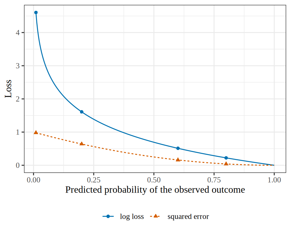
Figure 5: The log loss and the squared error of Example 4 for a positive case, as the probability given to the positive class moves from 0 to 1, with the four values of the example marked. The squared error stays below 1, while the log loss grows without bound as the probability approaches 0.
(a)
Line plot of two losses for an observation whose outcome is 1, against the predicted probability from 0 to 1. The solid curve, the log loss, is very large near probability 0, about 4.6 at 0.01, and falls to 0 at probability 1. The dashed curve, the squared error, falls from 1 at probability 0 to 0 at probability 1 and never exceeds 1. Four marked points sit on each curve at the predicted probabilities 0.01, 0.2, 0.6 and 0.8.
(b)
Line plot of two losses for an observation whose outcome is 1, against the predicted probability from 0 to 1. The solid curve, the log loss, is very large near probability 0, about 4.6 at 0.01, and falls to 0 at probability 1. The dashed curve, the squared error, falls from 1 at probability 0 to 0 at probability 1 and never exceeds 1. Four marked points sit on each curve at the predicted probabilities 0.01, 0.2, 0.6 and 0.8.

Theorem 1 (Binary form of the log loss)

Theorem 1 (Binary form of the log loss) For a label \(\outvar_i \in \set{0, 1}\) and a predicted probability \(\prob_i \in (0, 1)\), the log loss is

\[ C_i = -\outvar_i \log \prob_i - (1 - \outvar_i) \log (1 - \prob_i). \]

Proof

Proof. The model gives probability \(\prob_i\) to label \(1\) and \(1 - \prob_i\) to label \(0\). Because \(\outvar_i \in \set{0, 1}\), the observed label is one of the two:

  • Case \(\outvar_i = 1\): \(C_i = -\log \prob_i\). This is the formula, because \(1 - \outvar_i = 0\).
  • Case \(\outvar_i = 0\): \(C_i = -\log (1 - \prob_i)\). This is the formula, because \(\outvar_i = 0\).

Example 5 (Binary form of the log loss for a label of zero)

Example 5 (Binary form of the log loss for a label of zero) Suppose \(\outvar_i = 0\), and the model predicts \(\prob_i = 0.8\). The model gives probability \(1 - 0.8 = 0.2\) to the observed label, so the log loss is \(C_i = -\log 0.2\). The formula of Theorem 1 gives the same value,

\[ C_i = -0 \cdot \log 0.8 - (1 - 0) \log (1 - 0.8) = -\log 0.2. \]

Definition 2 (Cross-entropy loss)

Definition 2 (Cross-entropy loss) For a label \(\outvar_i \in \set{1, \dots, K}\) and a model that predicts the probability \(q_{ik} = \Prf{\Outvar_i = k \mid \vpredvar_i}\) of each value \(k\), let \(\vq_i = (q_{i1}, \dots, q_{iK})\) be the model’s distribution, and let \(\vp_i\) be the distribution that puts probability \(1\) on the observed label, so \(p_{ik} = 1\) when \(k = \outvar_i\), and \(p_{ik} = 0\) otherwise. The per-observation cross-entropy loss is the cross-entropy of \(\vq_i\) relative to \(\vp_i\),

\[ H(\vp_i, \vq_i). \]

For a binary label coded \(0\) and \(1\), the two entries of each vector are listed in that order.

Example 6 (Label and model distributions for one observation)

Example 6 (Label and model distributions for one observation) Suppose \(\outvar_i = 1\), and the model predicts \(\prob_i = 0.8\). The distribution of the observed label is \(\vp_i = (0, 1)\), and the model’s distribution is \(\vq_i = (0.2, 0.8)\). The cross-entropy loss is

\[ H(\vp_i, \vq_i) = -0 \cdot \log 0.2 - 1 \cdot \log 0.8 = -\log 0.8, \]

where the term with probability \(0\) is taken to be \(0\).

Figure 6 plots both cases.

Show code
cel_labels <- c("label 1", "label 0")
cel_label <- rep(cel_labels, each = 4)
cel_zero_one <- c(0, 1)
cel_outcome_raw <- rep(cel_zero_one, times = 4)
cel_outcome <- factor(cel_outcome_raw)
cel_sources <- c("label", "model")
cel_who_once <- rep(cel_sources, each = 2)
cel_who <- rep(cel_who_once, times = 2)
cel_mass <- c(0, 1, 0.2, 0.8, 1, 0, 0.2, 0.8)
cel_panel <- factor(cel_label, levels = cel_labels)
cel_fig <- tibble::tibble(
  label = cel_panel,
  outcome = cel_outcome,
  who = cel_who,
  mass = cel_mass
)
cel_fills <- c(label = "#D55E00", model = "#0072B2")
cel_fig |>
  ggplot2::ggplot(ggplot2::aes(outcome, mass, fill = who)) +
  ggplot2::geom_col(position = "dodge", width = 0.7) +
  ggplot2::facet_wrap(~label) +
  ggplot2::scale_fill_manual(values = cel_fills) +
  ggplot2::labs(x = "Outcome", y = "Probability", fill = NULL)
Show code
import matplotlib.pyplot as plt
import numpy as np

fig, axes = plt.subplots(1, 2, figsize=(6, 3), sharey=True, layout="constrained")
pos_cel = np.arange(2)
for ax, title, p_label in zip(axes, ["label 1", "label 0"], [[0, 1], [1, 0]]):
    ax.bar(pos_cel - 0.18, p_label, width=0.36, color="#D55E00", label="label");
    ax.bar(pos_cel + 0.18, [0.2, 0.8], width=0.36, color="#0072B2", label="model");
    ax.set_xticks(pos_cel, ["0", "1"]);
    ax.set_title(title);
    ax.set_xlabel("Outcome");
axes[0].set_ylabel("Probability");
axes[1].legend();
plt.show()
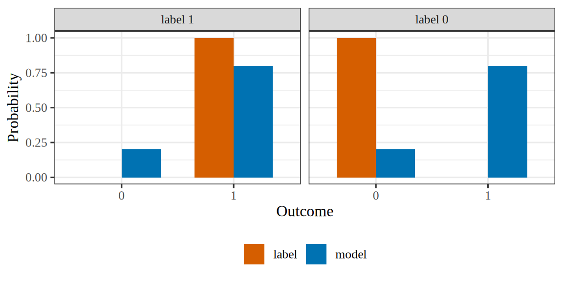
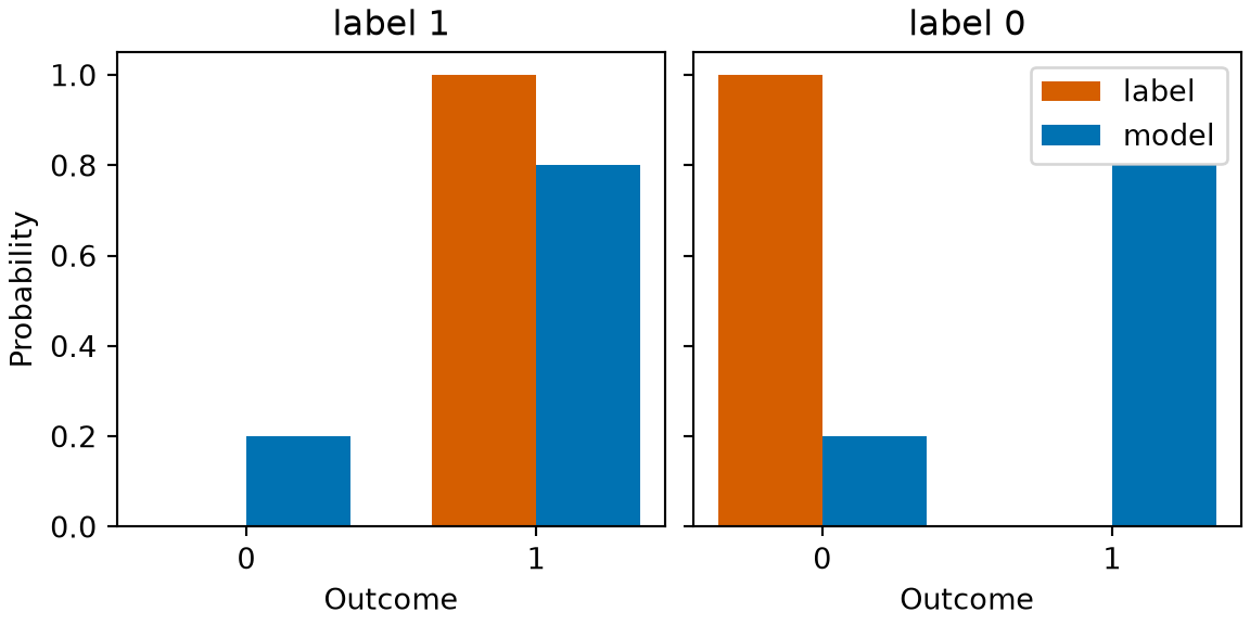
Figure 6: The distribution of the label (vermilion) and of the model (blue) over the two outcomes, for a label of \(1\) and a label of \(0\), with the model’s probability \(0.8\).
(a)
Two panels of paired bars over the outcomes 0 and 1. In the panel for a label of 1, the vermilion bars of the label's distribution are 0 at the outcome 0 and 1 at the outcome 1, and the blue bars of the model's distribution are 0.2 and 0.8. In the panel for a label of 0, the label's bars are 1 and 0, and the model's bars are again 0.2 and 0.8.
(b)
Two panels of paired bars over the outcomes 0 and 1. In the panel for a label of 1, the vermilion bars of the label's distribution are 0 at the outcome 0 and 1 at the outcome 1, and the blue bars of the model's distribution are 0.2 and 0.8. In the panel for a label of 0, the label's bars are 1 and 0, and the model's bars are again 0.2 and 0.8.

Theorem 2 (The cross-entropy loss equals the log loss)

Theorem 2 (The cross-entropy loss equals the log loss) For a label \(\outvar_i \in \set{1, \dots, K}\), the cross-entropy loss equals the log loss,

\[ H(\vp_i, \vq_i) = C_i. \]

Proof

Proof. Let \(\vp_i\) and \(\vq_i\) be as in the definition. By the definition of cross-entropy,

\[ \begin{aligned} H(\vp_i, \vq_i) &= -\sumto{k}{K} p_{ik} \log q_{ik} && \text{(definition of cross-entropy)} \\ &= -\log q_{i \outvar_i} && \text{($p_{ik} = 0$ unless $k = \outvar_i$, and $p_{i \outvar_i} = 1$)} \\ &= -\log \Prf{\Outvar_i = \outvar_i \mid \vpredvar_i} && \text{(definition of $q_{ik}$)} \\ &= C_i. \end{aligned} \]

The last line is the definition of the log loss.

Example 7 (The cross-entropy loss equals the log loss for a label of zero)

Example 7 (The cross-entropy loss equals the log loss for a label of zero) Suppose \(\outvar_i = 0\), and the model predicts \(\prob_i = 0.8\). Then \(\vp_i = (1, 0)\) and \(\vq_i = (0.2, 0.8)\), so the cross-entropy loss is

\[ H(\vp_i, \vq_i) = -1 \cdot \log 0.2 - 0 \cdot \log 0.8 = -\log 0.2. \]

This equals the log loss \(C_i = -\log 0.2\) of Example 5.

The right panel of Figure 6 plots this case.

Definition 3 (Total log loss)

Definition 3 (Total log loss) For labels \(\outvar_1, \dots, \outvar_n\) and predicted probabilities \(\prob_1, \dots, \prob_n\) determined by the coefficients \(\vcoef\), the total log loss is the sum of the per-observation log losses,

\[ \begin{aligned} C(\vcoef) &= \sumin C_i \\ &= \sumin \sb{ -\outvar_i \log \prob_i - (1 - \outvar_i) \log (1 - \prob_i) }. \end{aligned} \]

Example 8 (Total log loss of the type A men under one shared probability)

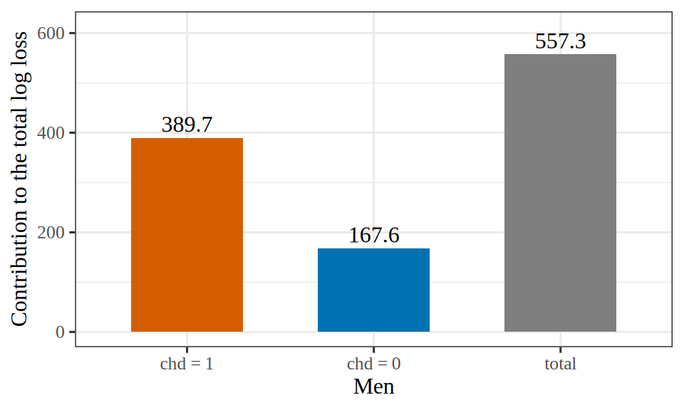
Example 8 (Total log loss of the type A men under one shared probability) Consider the WCGS data of the exercise on why not a line (data/wcgs.csv), whose column dibpat records each man’s behavior pattern, type A or type B, and subset to the men of type A (dibpat is "A"). Model coronary heart disease (chd) on age at enrollment with \(\prob_i = \sigmoidf{\coef{0} + \coef{1}\,\text{age}_i}\), and take the coefficients \(\coef{1} = 0\) and \(\coef{0}\) chosen so that every man gets the same probability \(\outbar\), the proportion of these men with chd equal to 1. Evaluate each man’s log loss \(C_i\) and the total log loss \(C(\vcoef)\):

wcgs_a <- subset(read.csv("data/wcgs.csv"), dibpat == "A")
chd_a <- wcgs_a$chd
p_bar <- mean(chd_a)
loss_i <- -chd_a * log(p_bar) - (1 - chd_a) * log(1 - p_bar)
round(c(
  n = length(loss_i),
  loss_if_chd = -log(p_bar),
  loss_if_no_chd = -log(1 - p_bar),
  total = sum(loss_i)
), 3)
             n    loss_if_chd loss_if_no_chd          total 
      1589.000          2.189          0.119        557.291 
import numpy as np
import pandas as pd

wcgs_all = pd.read_csv("data/wcgs.csv")
wcgs_a = wcgs_all[wcgs_all["dibpat"] == "A"]
chd_a = wcgs_a["chd"].to_numpy(float)
p_bar = chd_a.mean()
loss_i = -chd_a * np.log(p_bar) - (1.0 - chd_a) * np.log(1.0 - p_bar)
print(pd.Series({
    "n": len(loss_i),
    "loss_if_chd": -np.log(p_bar),
    "loss_if_no_chd": -np.log(1.0 - p_bar),
    "total": loss_i.sum(),
}).round(3))
n                 1589.000
loss_if_chd          2.189
loss_if_no_chd       0.119
total              557.291
dtype: float64

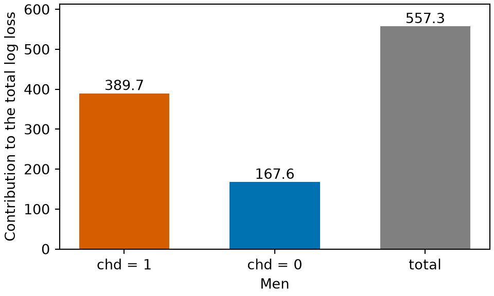
Here \(\outbar = 0.112\). Each of the 178 men with chd equal to 1 contributes \(-\log \outbar = 2.189\), and each of the other 1411 contributes \(-\log(1 - \outbar) = 0.119\), so the total log loss is 557.3.

Figure 7 plots the two contributions and their total.

Show code
tll_n1 <- sum(chd_a)
tll_n0 <- sum(1 - chd_a)
tll_contrib <- c(tll_n1 * -log(p_bar), tll_n0 * -log(1 - p_bar))
tll_total <- sum(tll_contrib)
tll_values <- c(tll_contrib, tll_total)
tll_shown <- round(tll_values, 1)
tll_names <- c("chd = 1", "chd = 0", "total")
tll_what <- factor(tll_names, levels = tll_names)
tll_fig <- tibble::tibble(what = tll_what, value = tll_values)
tll_fills <- c("chd = 1" = "#D55E00", "chd = 0" = "#0072B2", total = "grey50")
tll_limits <- c(0, 1.1 * tll_total)
tll_fig |>
  ggplot2::ggplot(ggplot2::aes(what, value, fill = what)) +
  ggplot2::geom_col(width = 0.6) +
  ggplot2::geom_text(ggplot2::aes(label = tll_shown), vjust = -0.4) +
  ggplot2::scale_fill_manual(values = tll_fills, guide = "none") +
  ggplot2::scale_y_continuous(limits = tll_limits) +
  ggplot2::labs(x = "Men", y = "Contribution to the total log loss")
Show code
import matplotlib.pyplot as plt
import numpy as np

contrib_tll = [chd_a.sum() * -np.log(p_bar), (1 - chd_a).sum() * -np.log(1 - p_bar)]
fig, ax = plt.subplots(figsize=(5, 3), layout="constrained")
bars_tll = ax.bar(["chd = 1", "chd = 0", "total"], [*contrib_tll, sum(contrib_tll)],
                  color=["#D55E00", "#0072B2", "grey"], width=0.6);
ax.bar_label(bars_tll, fmt="%.1f");
ax.set_ylim(0, 1.1 * sum(contrib_tll));
ax.set_xlabel("Men");
ax.set_ylabel("Contribution to the total log loss");
plt.show()
Figure 7: The contribution of the men with chd equal to 1 (vermilion) and equal to 0 (blue) to the total log loss of Example 8, and the total (gray).
(a)
Bar chart of three totals of the log loss for the type A men. A vermilion bar for the men with chd equal to 1 and a blue bar for the men with chd equal to 0 show each group's contribution, and a grey bar shows the total, which equals the sum of the other two.
(b)
Bar chart of three totals of the log loss for the type A men. A vermilion bar for the men with chd equal to 1 and a blue bar for the men with chd equal to 0 show each group's contribution, and a grey bar shows the total, which equals the sum of the other two.

Remark 1 (Per-observation, total and average log loss)

Remark 1 (Per-observation, total and average log loss). The average of the total log loss, \(\empriskf{\vcoef} = \tfrac{1}{n} C(\vcoef)\), is the empirical risk under the log loss. Different sources apply the name log loss or cross-entropy loss to the per-observation loss function \(\lossf{\outvar_i, \prob_i}\), to the sum \(C(\vcoef)\), or to the average \(\empriskf{\vcoef}\) [1]. Because the cross-entropy loss equals the log loss (Theorem 2), the sum of the cross-entropy losses equals the total log loss.

Proposition 1 (The total log loss is the negative log-likelihood)

Proposition 1 (The total log loss is the negative log-likelihood) Under the assumptions of Lemma 2, the total log loss is the negative log-likelihood:

\[C(\vcoef) = -\llik(\vcoef).\]

Proof

Proof. By Definition 3,

\[ \begin{aligned} C(\vcoef) &= \sumin \sb{ -\outvar_i \log \prob_i - (1 - \outvar_i) \log (1 - \prob_i) } \\ &= -\sumin \sb{ \outvar_i \log \prob_i + (1 - \outvar_i) \log (1 - \prob_i) }, \end{aligned} \]

and the last sum is \(\llik(\vcoef)\) by Lemma 3.

Example 9 (The log-likelihood a fitting function reports is the negative total log loss)

Example 9 (The log-likelihood a fitting function reports is the negative total log loss) For the type A men of Example 8, fit two logistic regressions of chd, one with an intercept only and one on age. For each fit, compute the total log loss of its fitted probabilities, and compare it with the log-likelihood the software reports:

fit_const <- glm(chd ~ 1, family = binomial, data = wcgs_a)
fit_age <- glm(chd ~ age, family = binomial, data = wcgs_a)

total_log_loss <- function(fit) {
  p <- fitted(fit)
  y <- fit$y
  sum(-y * log(p) - (1 - y) * log(1 - p))
}

loglik_check <- data.frame(
  total_log_loss = c(total_log_loss(fit_const), total_log_loss(fit_age)),
  neg_loglik = -c(as.numeric(logLik(fit_const)), as.numeric(logLik(fit_age))),
  row.names = c("intercept_only", "age")
)
round(loglik_check, 4)
import statsmodels.api as sm

designs = {
    "intercept_only": np.ones((len(chd_a), 1)),
    "age": sm.add_constant(wcgs_a["age"].to_numpy(float)),
}
rows = {}
for name, x in designs.items():
    fit = sm.GLM(chd_a, x, family=sm.families.Binomial()).fit()
    p = fit.predict()
    rows[name] = {
        "total_log_loss": np.sum(-chd_a * np.log(p) - (1.0 - chd_a) * np.log(1.0 - p)),
        "neg_loglik": -fit.llf,
    }
print(pd.DataFrame(rows).T.round(4))
                total_log_loss  neg_loglik
intercept_only        557.2912    557.2912
age                   543.5083    543.5083

In both rows, and in both languages, the two columns agree, as Proposition 1 states. The intercept-only fit gives every man the probability \(\outbar\), so its row repeats the total of Example 8. Adding age lowers the total log loss to 543.5.

Theorem 3 (Minimizing the log loss is maximum likelihood estimation)

Theorem 3 (Minimizing the log loss is maximum likelihood estimation) Suppose the outcomes \(\Outvar_1, \dots, \Outvar_n \in \set{0, 1}\) are conditionally independent given \(\vpredvar_1, \dots, \vpredvar_n\), with

\[ \Outvar_i \mid \vpredvar_i \sim \Bernoulli\paren{\prob_i}, \qquad \prob_i = \sigmoidf{\dprod{\vcoef}{\vpredvar_i}}. \]

Then minimizing the total log loss \(C(\vcoef)\) (or the empirical risk \(\empriskf{\vcoef} = \tfrac{1}{n} C(\vcoef)\)) with respect to \(\vcoef\) gives the maximum likelihood estimate \(\hvcoef\). The log loss is therefore the plausible loss for conditionally independent Bernoulli outcomes.

Proof

Proof. By assumption, the outcomes are conditionally independent with \(\Outvar_i \mid \vpredvar_i \sim \Bernoulli\paren{\prob_i}\), so Lemma 2 gives the likelihood and Lemma 3 gives the log-likelihood \(\llik(\vcoef)\), which is \(-C(\vcoef)\) by Proposition 1. Because \(\log\) is strictly increasing, maximizing the likelihood is equivalent to maximizing \(\llik(\vcoef)\), which is equivalent to minimizing \(C(\vcoef)\). Because \(n > 0\), minimizing \(C(\vcoef)\) is equivalent to minimizing \(\tfrac{1}{n} C(\vcoef)\).

Example 10 (Minimizing the log loss on the WCGS data gives the maximum likelihood fit)

Example 10 (Minimizing the log loss on the WCGS data gives the maximum likelihood fit) Consider again the type A men of the WCGS data, as in Example 8, so that a single curve with two coefficients describes them. Model coronary heart disease (chd) on age at enrollment (age) with \(\prob_i = \sigmoidf{\coef{0} + \coef{1}\,\text{age}_i}\). Minimize the average log loss (empirical risk) \(\empriskf{\vcoef} = \tfrac{1}{n} C(\vcoef)\) numerically from \(\vcoef = \vzero\), and compare with the maximum likelihood fit:

wcgs_mle <- subset(read.csv("data/wcgs.csv"), dibpat == "A")
y_wcgs <- wcgs_mle$chd
x_wcgs <- cbind(1, wcgs_mle$age)

mean_log_loss <- function(b) {
  p <- plogis(drop(x_wcgs %*% b))
  mean(-y_wcgs * log(p) - (1 - y_wcgs) * log(1 - p))
}

loss_fit <- optim(c(0, 0), mean_log_loss, control = list(reltol = 1e-14))
glm_fit <- coef(glm(chd ~ age, family = binomial, data = wcgs_mle))
round(rbind(log_loss_minimizer = loss_fit$par, mle = unname(glm_fit)), 6)
                        [,1]     [,2]
log_loss_minimizer -5.498861 0.071907
mle                -5.498862 0.071907
import numpy as np
import pandas as pd
import statsmodels.api as sm
from scipy.optimize import minimize
from scipy.special import expit

wcgs_all = pd.read_csv("data/wcgs.csv")
wcgs_mle = wcgs_all[wcgs_all["dibpat"] == "A"]
y_wcgs = wcgs_mle["chd"].to_numpy(float)
x_wcgs = sm.add_constant(wcgs_mle["age"].to_numpy(float))

def mean_log_loss(b):
    p = expit(x_wcgs @ b)
    return np.mean(-y_wcgs * np.log(p) - (1.0 - y_wcgs) * np.log(1.0 - p))

loss_fit = minimize(
    mean_log_loss,
    x0=np.zeros(2),
    method="Nelder-Mead",
    options={"xatol": 1e-10, "fatol": 1e-14},
)
glm_fit = sm.GLM(y_wcgs, x_wcgs, family=sm.families.Binomial()).fit().params
print(pd.DataFrame({"intercept": [loss_fit.x[0], glm_fit[0]],
                    "age": [loss_fit.x[1], glm_fit[1]]},
                   index=["log_loss_minimizer", "mle"]).round(6))
                    intercept       age
log_loss_minimizer  -5.498862  0.071907
mle                 -5.498862  0.071907

The numerical minimizer of \(\empriskf{\vcoef}\) and the maximum likelihood estimate differ by at most 3.4e-07, as Theorem 3 states.

Figure 8 plots the average log loss against the coefficient of age at enrollment.

Show code
library(ggplot2)
llm_slopes <- seq(0.03, 0.115, length.out = 111)
llm_curve <- data.frame(
  slope = llm_slopes,
  loss = vapply(llm_slopes, \(s) mean_log_loss(c(glm_fit[[1]], s)), numeric(1))
)
llm_pt <- data.frame(slope = loss_fit$par[2], loss = mean_log_loss(loss_fit$par))
ggplot(llm_curve, aes(slope, loss)) +
  geom_line(colour = "#0072B2") +
  geom_vline(xintercept = glm_fit[[2]], linetype = "dashed", colour = "#D55E00") +
  geom_point(data = llm_pt, colour = "#D55E00", shape = 17, size = 3) +
  labs(x = "Coefficient of age at enrollment", y = "Average log loss")
Show code
import matplotlib.pyplot as plt
import numpy as np

slopes_llm = np.linspace(0.03, 0.115, 111)
loss_llm = [mean_log_loss(np.array([glm_fit[0], s])) for s in slopes_llm]
fig, ax = plt.subplots(figsize=(6, 4), layout="constrained")
ax.plot(slopes_llm, loss_llm, color="#0072B2");
ax.axvline(glm_fit[1], color="#D55E00", linestyle="--");
ax.plot(loss_fit.x[1], mean_log_loss(loss_fit.x), color="#D55E00", marker="^", markersize=8,
        linestyle="");
ax.set_xlabel("Coefficient of age at enrollment");
ax.set_ylabel("Average log loss");
plt.show()
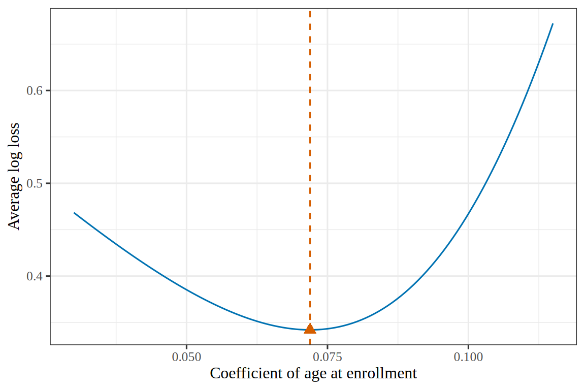
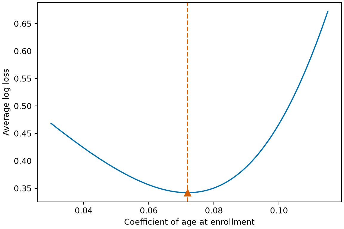
Figure 8: The average log loss of Example 10, for the type A men, as the coefficient of age at enrollment varies, with the intercept held at its fitted value. The numerical minimizer (triangle) and the maximum likelihood coefficient (dashed line) coincide.
(a)
Plot of the average log loss for the type A men in the WCGS data against the coefficient of age at enrollment, with the intercept held at its fitted value. A solid blue U-shaped curve has its lowest point at the fitted coefficient, near 0.072, with a minimum average loss of about 0.34. A vermilion triangle marks the minimizer found numerically, and a dashed vermilion vertical line marks the maximum likelihood coefficient. The marker and the line are at the same coefficient.
(b)
Plot of the average log loss for the type A men in the WCGS data against the coefficient of age at enrollment, with the intercept held at its fitted value. A solid blue U-shaped curve has its lowest point at the fitted coefficient, near 0.072, with a minimum average loss of about 0.34. A vermilion triangle marks the minimizer found numerically, and a dashed vermilion vertical line marks the maximum likelihood coefficient. The marker and the line are at the same coefficient.

Exercise 10 (The same loss, written two ways)

Exercise 10 (The same loss, written two ways) Exercise 3 gave the per-observation cost with labels \(y \in \{0, 1\}\):

\[C(\logodds, y) = -y\log\sigmoid(\logodds) - (1-y)\log\paren{1 - \sigmoid(\logodds)}, \qquad \logodds = \dprod{\vcoef}{\vx}\]

Much of the literature instead uses the labels \(\signoutvar \in \{-1, +1\}\), with \(\signoutvar = 2y - 1\).

Show that \(C(\logodds, y) = \log\paren{1 + \e{-\signoutvar \logodds}}\).

Solution 10. Check the two cases \(y = 1\) and \(y = 0\) separately. The steps use the definition \(\sigmoid(\logodds) = 1 / \paren{1 + \e{-\logodds}}\).

If \(y = 1\), then \(\signoutvar = +1\), and

\[ \begin{aligned} C(\logodds, 1) &= -1 \cdot \log\sigmoid(\logodds) - 0 \cdot \log\paren{1 - \sigmoid(\logodds)} && \text{(substitute } y = 1\text{)} \\ &= -\log\sigmoid(\logodds) && \text{(the second term equals } 0\text{)} \\ &= -\log\frac{1}{1 + \e{-\logodds}} && \text{(definition of } \sigmoid\text{)} \\ &= \log\paren{1 + \e{-\logodds}} && \text{(}\log(1/a) = -\log a\text{)} \\ &= \log\paren{1 + \e{-\signoutvar \logodds}} && \text{(}\signoutvar = 1\text{)}. \end{aligned} \]

If \(y = 0\), then \(\signoutvar = -1\). The identity \(1 - \sigmoid(\logodds) = \sigmoid(-\logodds)\) from part 2 of the sigmoid properties exercise gives

\[ \begin{aligned} C(\logodds, 0) &= -0 \cdot \log\sigmoid(\logodds) - 1 \cdot \log\paren{1 - \sigmoid(\logodds)} && \text{(substitute } y = 0\text{)} \\ &= -\log\paren{1 - \sigmoid(\logodds)} && \text{(the first term equals } 0\text{)} \\ &= -\log\sigmoid(-\logodds) && \text{(}1 - \sigmoid(\logodds) = \sigmoid(-\logodds)\text{)} \\ &= -\log\frac{1}{1 + \e{\logodds}} && \text{(definition of } \sigmoid\text{)} \\ &= \log\paren{1 + \e{\logodds}} && \text{(}\log(1/a) = -\log a\text{)} \\ &= \log\paren{1 + \e{-\signoutvar \logodds}} && \text{(}\signoutvar = -1\text{)}. \end{aligned} \]

Both cases give the same expression, so the two formulas are the same loss function written under two label conventions. Under the \(\{-1, +1\}\) convention, the loss depends on \(\logodds\) and \(\signoutvar\) only through their product \(\signoutvar \logodds\).

Definition 4 (Margin of an observation)

Definition 4 (Margin of an observation) The margin of an observation with label \(y \in \set{0, 1}\) and log-odds \(\logodds = \dprod{\vcoef}{\vx}\) is

\[ m \eqdef \signoutvar \logodds, \qquad \signoutvar = 2y - 1 \in \set{-1, +1}. \]

Example 11 (Margins of a man with a body mass index of 25)

Example 11 (Margins of a man with a body mass index of 25) In the model of the logistic function example, a man with \(\text{bmi} = 25\) has the log-odds \(\logodds = -2.402\). If he has coronary heart disease, then \(\signoutvar = +1\), and his margin is \(m = -2.402\), which is negative because his log-odds puts him on the side of the decision boundary where the model predicts no disease. If he does not have the disease, then \(\signoutvar = -1\), and his margin is \(m = 2.402\), which is positive.

Remark 2 (Reading the margin)

Remark 2 (Reading the margin). The label \(\signoutvar\) is the label \(y\) recoded from \(0\) and \(1\) to \(-1\) and \(+1\) (Exercise 10), and the tilde keeps it distinct from \(y\). The margin is positive when the log-odds and the label have the same sign, so that the observation is on the correct side of the decision boundary \(\logodds = 0\), and negative when it is on the wrong side. Its absolute value \(\abs{m} = \abs{\logodds}\) is the distance of the log-odds from \(0\). The margin of a separating hyperplane, in the chapter on support vector machines, is a different quantity.

Exercise 11 (The same loss, written two ways (part 2))

Exercise 11 (The same loss, written two ways (part 2)) Use the setup of Exercise 10.

Let \(m = \signoutvar \logodds\) be the margin. Describe \(\log(1 + \e{-m})\) as a function of \(m\): its monotonicity, its value at \(m = 0\), and its behavior as \(m \to +\infty\) and as \(m \to -\infty\).

Solution 11. As a function of \(m\), \(\log(1 + \e{-m})\) is strictly decreasing, because \(\e{-m}\) is strictly decreasing and \(\log\) is strictly increasing. A larger margin always gives a smaller loss, so the loss orders observations by their margins.

At \(m = 0\) the loss is \(\log 2\), which is the log loss of predicting the probability \(\tfrac12\) for the observed label.

As \(m \to +\infty\), the loss decreases to \(0\), but it is strictly positive for every finite \(m\). Increasing the margin of a correctly classified observation therefore always reduces the loss a little.

As \(m \to -\infty\), the \(1\) in \(1 + \e{-m}\) becomes negligible, so \(\log(1 + \e{-m}) \approx \log \e{-m}\), which equals \(-m\). The loss therefore increases linearly with the size of a negative margin, whereas the least-squares loss \((1 - m)^2\) on the log-odds increases quadratically. A single badly misclassified observation therefore has a bounded effect on the gradient under the log loss, and an unbounded effect under least squares on the log-odds.

Exercise 12 (The same loss, written two ways (part 2b))

Exercise 12 (The same loss, written two ways (part 2b)) Use the setup of Exercise 10.

Give the values of \(\log(1 + \e{-m})\) at \(m = 0\) and at \(m = \pm 2\) to three significant figures.

Solution 12. This continues Solution 11.

Show code
tlc_m <- c(-2, 0, 2)
tlc_exp <- exp(-tlc_m)
tlc_loss <- log1p(tlc_exp)
tlc_shown <- formatC(tlc_loss, digits = 3, format = "fg", flag = "#")
tlc_table <- tibble::tibble(m = tlc_m, loss = tlc_shown)
tlc_cols <- c("$m$", "$\\log(1 + \\e{-m})$")
knitr::kable(tlc_table, col.names = tlc_cols)
\(m\) \(\log(1 + \e{-m})\)
-2 2.13
0 0.693
2 0.127

Exercise 13 (The same loss, written two ways (part 3))

Exercise 13 (The same loss, written two ways (part 3)) Use the setup of Exercise 10.

The hinge loss \(\max(0,\, 1 - m)\) is the loss that support vector machines use. State one property that the hinge loss has and the logistic loss does not.

Solution 13. The hinge loss \(\max(0, 1 - m)\) equals \(0\) for every \(m \ge 1\). Observations with margin greater than \(1\) contribute zero gradient, so the fitted decision boundary of a support vector machine depends only on the observations with \(m \le 1\), the support vectors.

Exercise 14 (The same loss, written two ways (part 3b))

Exercise 14 (The same loss, written two ways (part 3b)) Use the setup of Exercise 10.

State one property that the logistic loss has and the hinge loss does not.

Solution 14. This continues Solution 13.

The log loss is strictly positive for every finite \(m\), so every observation contributes to the fit, with a gradient weight \(\sigmoid(-m)\) that decreases exponentially as \(m \to +\infty\). It has derivatives of every order everywhere, whereas the hinge loss has a corner at \(m = 1\) where it is not differentiable, so fitting it needs subgradient methods or constrained quadratic programming. The log loss is also the negative log-likelihood of a Bernoulli model, so minimizing it gives estimates \(\sigmoid(\logodds)\) of the probabilities, which are accurate when that model is correct. A support vector machine gives a linear function of the features, and converting the linear function to a probability needs a separate step after the fit.

Exercise 15 (The same loss, written two ways (part 4))

Exercise 15 (The same loss, written two ways (part 4)) Use the setup of Exercise 10.

The error rate of a classifier is often the quantity of interest, and its per-observation cost is the zero–one loss \(\truthindf{m \le 0}\). Explain why it is not used for fitting.

Solution 15. The zero–one loss \(\truthindf{m \le 0}\) takes only the values \(0\) and \(1\), so it is constant in \(\vcoef\) except where some margin crosses \(0\). Its derivative with respect to \(\vcoef\) is zero wherever it exists, and it does not exist where \(m = 0\), so the gradient gives no direction in which to change \(\vcoef\). The zero–one loss is also not convex, and minimizing the number of misclassified training points over classifiers with a hyperplane boundary is NP-hard, even approximately [2], abstract.

Exercise 16 (The same loss, written two ways (part 4b))

Exercise 16 (The same loss, written two ways (part 4b)) Use the setup of Exercise 10.

Show that

\[\truthindf{m \le 0} \le \frac{1}{\log 2}\,\log\paren{1 + \e{-m}} \quad\text{for every } m.\]

Solution 16. This continues Solution 15.

To verify the upper bound, check the two cases \(m \le 0\) and \(m > 0\):

  • If \(m \le 0\), the left-hand side is \(1\). Because \(\e{-m} \ge 1\), \(\log(1 + \e{-m}) \ge \log 2\), so the right-hand side is at least \(\log 2 / \log 2\), which equals \(1\).
  • If \(m > 0\), the left-hand side is \(0\), and the right-hand side is positive because \(1 + \e{-m} > 1\).

The inequality therefore holds for every \(m \in \reals\).

Exercise 17 (The same loss, written two ways (part 4c))

Exercise 17 (The same loss, written two ways (part 4c)) Use the setup of Exercise 10.

Explain what reducing the right-hand side of the inequality of Exercise 16 therefore gains.

Solution 17. This continues Solution 15.

Averaging the inequality of Solution 16 over the training set shows that the mean log loss divided by \(\log 2\) is an upper bound on the error rate on the training set. Minimizing the log loss therefore minimizes a differentiable, convex upper bound on the error rate on the training set, which is called a surrogate for the zero–one loss.

The bound is not tight for positive margins. At \(m = 2\), the rescaled log loss is \(\log(1 + \e{-2}) / \log 2 = 0.183\), although the zero–one loss is \(0\). A fit can therefore reduce its log loss by increasing positive margins without changing any classification.

Theorem 4 (The log loss depends on the margin alone)

Theorem 4 (The log loss depends on the margin alone) Let \(y \in \{0, 1\}\), \(\signoutvar = 2y - 1 \in \{-1, +1\}\) and \(\logodds = \dprod{\vcoef}{\vx}\). Then the per-observation log loss,

\[ \lossf{y, \sigmoid(\logodds)} = -y\log\sigmoid(\logodds) - (1-y)\log\paren{1 - \sigmoid(\logodds)}, \]

equals \(\log\paren{1 + \e{-m}}\), where \(m = \signoutvar \logodds\) is the margin. This loss is strictly decreasing in \(m\).

Proof

Proof. The equality is Solution 10, and the monotonicity is Solution 11.

Example 12 (Evaluating the log loss from the log-odds and from the margin)

Example 12 (Evaluating the log loss from the log-odds and from the margin) Consider the log-odds \(\logodds = 2\), so \(\prob = \sigmoid(2)\) is 0.881, and compare the log loss under the two labels: \(y = 1\), with \(\signoutvar = +1\) and margin \(m = +2\), and \(y = 0\), with \(\signoutvar = -1\) and margin \(m = -2\).

z_mf <- 2
y_mf <- c(1, 0)
y_tilde_mf <- 2 * y_mf - 1
m_mf <- y_tilde_mf * z_mf
p_mf <- plogis(z_mf)

from_prob <- -y_mf * log(p_mf) - (1 - y_mf) * log(1 - p_mf)
from_margin <- log1p(exp(-m_mf))
round(data.frame(y = y_mf, y_tilde = y_tilde_mf, margin = m_mf,
                 from_prob = from_prob, from_margin = from_margin), 3)
import numpy as np
import pandas as pd
from scipy.special import expit

z_mf = 2.0
y_mf = np.array([1, 0])
y_tilde_mf = 2 * y_mf - 1
m_mf = y_tilde_mf * z_mf
p_mf = expit(z_mf)

print(pd.DataFrame({
    "y": y_mf,
    "y_tilde": y_tilde_mf,
    "margin": m_mf,
    "from_prob": -y_mf * np.log(p_mf) - (1 - y_mf) * np.log(1 - p_mf),
    "from_margin": np.log1p(np.exp(-m_mf)),
}).round(3))
   y  y_tilde  margin  from_prob  from_margin
0  1        1     2.0      0.127        0.127
1  0       -1    -2.0      2.127        2.127

Both formulas give 0.127 on the correctly classified observation (\(m = +2\)) and 2.13 on the misclassified one (\(m = -2\)).

Figure 9 compares four curves as functions of \(m\).

Show code
library(ggplot2)

m_grid <- seq(-2.5, 2.5, length.out = 501)
margin_df <- rbind(
  data.frame(
    m = m_grid,
    loss = log1p(exp(-m_grid)),
    kind = "Logistic: log(1 + exp(-m))"
  ),
  data.frame(
    m = m_grid,
    loss = pmax(0, 1 - m_grid),
    kind = "Hinge: max(0, 1 - m)"
  ),
  data.frame(
    m = m_grid,
    loss = (1 - m_grid)^2,
    kind = "Least squares: (1 - m)^2"
  ),
  data.frame(
    m = m_grid,
    loss = as.numeric(m_grid <= 0),
    kind = "Misclassification: 1[m <= 0]"
  )
)
margin_df$kind <- factor(
  margin_df$kind,
  levels = c(
    "Logistic: log(1 + exp(-m))",
    "Hinge: max(0, 1 - m)",
    "Least squares: (1 - m)^2",
    "Misclassification: 1[m <= 0]"
  )
)

logistic_pts <- data.frame(
  m = c(-2, 0, 2),
  loss = log1p(exp(-c(-2, 0, 2)))
)

ggplot(margin_df) +
  aes(m, loss, colour = kind, linetype = kind) +
  geom_vline(xintercept = 0, colour = "grey70", linetype = "dotted") +
  geom_line(linewidth = 0.8) +
  geom_point(
    data = logistic_pts,
    aes(m, loss),
    inherit.aes = FALSE,
    colour = "#7570b3",
    size = 2.4
  ) +
  scale_colour_manual(values = c(
    "Logistic: log(1 + exp(-m))" = "#7570b3",
    "Hinge: max(0, 1 - m)" = "#d95f02",
    "Least squares: (1 - m)^2" = "#1f78b4",
    "Misclassification: 1[m <= 0]" = "#1b9e77"
  )) +
  scale_linetype_manual(values = c(
    "Logistic: log(1 + exp(-m))" = "solid",
    "Hinge: max(0, 1 - m)" = "dashed",
    "Least squares: (1 - m)^2" = "dotdash",
    "Misclassification: 1[m <= 0]" = "longdash"
  )) +
  coord_cartesian(ylim = c(0, 4)) +
  guides(colour = guide_legend(nrow = 2), linetype = guide_legend(nrow = 2)) +
  labs(
    x = "Margin m = y_tilde * η",
    y = "Loss",
    colour = NULL,
    linetype = NULL
  ) +
  theme(legend.position = "bottom")
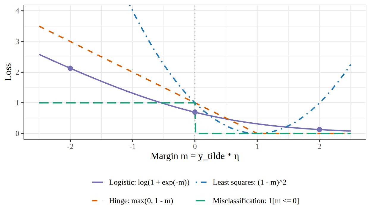
Figure 9: The log loss \(\log(1 + \e{-m})\), the hinge loss \(\max(0, 1 - m)\), the least-squares loss \((1 - m)^2\) and the misclassification loss \(\truthindf{m \le 0}\) as functions of the margin \(m = \signoutvar \logodds\). Dots mark the three log-loss values tabulated in Solution 12: \((-2, 2.13)\), \((0, 0.693)\) and \((2, 0.127)\).

Four loss curves plotted against the margin m from -2.5 to 2.5, with vertical axis from 0 to 4. The misclassification loss is a step at 1 for m at or below 0 and 0 for m above 0. The logistic loss falls smoothly from left to right, passing through marked dots at (-2, 2.13), (0, 0.693) and (2, 0.127), and approaching 0 without reaching it. The hinge loss falls linearly from 3.5 at m = -2.5 through 1 at m = 0 to 0 at m = 1, then stays at 0 for m >= 1. The least-squares parabola (1 - m)^2 touches 0 at m = 1 and rises steeply on both sides, penalizing margins above 1.

Remark 3 (The log loss and least squares, compared through their derivatives)

Remark 3 (The log loss and least squares, compared through their derivatives). Fitting the log-odds \(\logodds\) to \(\signoutvar \in \{-1, +1\}\) by least squares uses the loss \((\signoutvar - \logodds)^2\), which equals \((1 - m)^2\) because \(\signoutvar^2 = 1\). Its derivative with respect to \(\logodds\) is \(2(\logodds - \signoutvar)\). The derivative of the log loss \(\log(1 + \e{-\signoutvar \logodds})\) with respect to \(\logodds\) is \(-\signoutvar\,\sigmoid(-m)\).

Let \(\signoutvar = +1\):

  • at \(\logodds = -4\), a confidently wrong prediction, the log-loss derivative is \(-\sigmoid(4)\), which is -0.982, and the least-squares derivative is \(2(-4 - 1)\), which is -10;
  • at \(\logodds = 4\), a confidently correct prediction, the log-loss derivative is \(-\sigmoid(-4)\), which is -0.018, and the least-squares derivative is \(2(4 - 1)\), which is 6.

Squared error penalizes the prediction \(\logodds = 4\) because \(\logodds \ne \signoutvar\), although it is on the correct side of the decision boundary, and it gives large weight to observations with large negative margins. The log loss does neither. Figure 9 plots the log, hinge, squared-error and zero–one misclassification losses as functions of the margin \(m\).

Exercise 18 (Three names for the same optimization)

Exercise 18 (Three names for the same optimization) The fit of Exercise 3 can be described three ways, and different fields use different ones.

Starting from \(\argmax_{\vcoef}\llik(\vcoef)\), derive the other two formulations:

  • minimizing the negative log-likelihood, \(\argmin_{\vcoef}\ \sb{-\llik(\vcoef)}\);
  • empirical risk minimization, \(\argmin_{\vcoef}\empriskf{\vcoef}\), with \[\emprisk = \tfrac1\nobs\sumto{i}{\nobs} \lossf{\outvar_i, \prob_i}.\]

Solution 18. A point that maximizes \(\llik\) minimizes \(-\llik\), and dividing an objective by the positive constant \(n\) does not change its minimizer:

\[ \begin{aligned} \argmax_{\vcoef}\ \llik(\vcoef) &= \argmin_{\vcoef}\ \sb{-\llik(\vcoef)} && \text{(negate the objective)} \\ &= \argmin_{\vcoef}\ \sb{-\sum_i \paren{y_i\log\prob_i + (1-y_i)\log(1-\prob_i)}} && \text{(log-likelihood of the dataset)} \\ &= \argmin_{\vcoef}\ \sum_i \sb{-y_i\log\prob_i - (1-y_i)\log(1-\prob_i)} && \text{(move the minus sign into the sum)} \\ &= \argmin_{\vcoef}\ \frac1n \sum_i \sb{-y_i\log\prob_i - (1-y_i)\log(1-\prob_i)} && \text{(divide by } n > 0\text{)} \\ &= \argmin_{\vcoef}\ \frac1n \sum_i \lossf{y_i, \prob_i} && \text{(name the per-observation loss)}. \end{aligned} \]

The first line is maximum likelihood, the second and third minimize the negative log-likelihood, and the fourth and fifth are empirical risk minimization.

Exercise 19 (Three names for the same optimization (part 2))

Exercise 19 (Three names for the same optimization (part 2)) Use the setup of Exercise 18.

State the per-observation loss \(\lossf{\outvar_i, \prob_i}\).

Solution 19. The per-observation loss is

\[\lossf{y, \prob} = -y\log\prob - (1-y)\log(1-\prob),\]

the log loss, which equals the cross-entropy loss by Theorem 2. A later exercise in this series shows where the second name comes from.

Exercise 20 (Three names for the same optimization (part 3))

Exercise 20 (Three names for the same optimization (part 3)) Use the setup of Exercise 18.

Identify which step introduces the factor \(\tfrac1\nobs\).

Solution 20. In Solution 18, the factor \(\tfrac1n\) enters at the fourth line, the step that divides by \(n\), and nowhere else.

Exercise 21 (Three names for the same optimization (part 4))

Exercise 21 (Three names for the same optimization (part 4)) Use the setup of Exercise 18.

State what the factor \(\tfrac1\nobs\) changes and what it does not change.

Solution 21. Multiplying by \(\tfrac1n\) does not change the minimizer, because multiplying an objective by a positive constant does not change its argmin. It does not change the solutions of the score equations either, because those equations set a gradient equal to zero, and a gradient multiplied by \(\tfrac1n\) is zero exactly where the original gradient is zero.

The factor does change the scale of the gradient and of the second derivatives:

  • the size of the gradient, and so any step size tuned to it;
  • the second derivatives, and so any standard error computed from them. A standard error computed from the second derivatives of \(\tfrac1n C\) instead of \(C\) is too large by a factor of \(\sqrt n\).

Exercise 22 (Three names for the same optimization (part 5))

Exercise 22 (Three names for the same optimization (part 5)) Use the setup of Exercise 18.

For distributions \(\vp\) and \(\vq\) over the same outcomes, the cross-entropy is \(H(\vp, \vq) = -\sum_j p_j \log q_j\). Let \(\vp = (1 - \outvar,\; \outvar)\) be the distribution that puts all its probability on the observed label \(\outvar \in \{0, 1\}\), and let \(\vq = (1 - \prob,\; \prob)\).

Show that \(H(\vp, \vq)\) equals the per-observation loss of Exercise 18.

Solution 22. The two distributions are over the two outcomes \(\{0, 1\}\), so the sum has two terms:

\[ \begin{aligned} H(\vp, \vq) &= -p_0\log q_0 - p_1 \log q_1 && \text{(definition of cross-entropy)} \\ &= -(1 - y)\log(1 - \prob) - y\log\prob && \text{(substitute } \vp \text{ and } \vq\text{)} \\ &= \lossf{y, \prob} && \text{(the log loss)}. \end{aligned} \]

The log loss is therefore the cross-entropy between the distribution that puts all its probability on the observed label and the distribution that the model predicts, which is why it is also called the cross-entropy loss.

Exercise 23 (Three names for the same optimization (part 6))

Exercise 23 (Three names for the same optimization (part 6)) Use the setup of Exercise 18.

Show that \(H(\vp, \vq) \ge H(\vp, \vp)\) whenever \(q_j > 0\) for every \(j\) with \(p_j > 0\), with equality only when \(\vq = \vp\).

Solution 23. Terms with \(p_j = 0\) contribute \(0\) to both \(H(\vp, \vq)\) and \(H(\vp, \vp)\), by the convention \(0 \log 0 = 0\), so let \(S = \set{j : p_j > 0}\) and sum over \(S\) only. The difference of the two cross-entropies is

\[ \begin{aligned} H(\vp, \vq) - H(\vp, \vp) &= -\sum_{j \in S} p_j \log q_j + \sum_{j \in S} p_j \log p_j && \text{(definition of cross-entropy)} \\ &= \sum_{j \in S} p_j \paren{\log p_j - \log q_j} && \text{(combine the sums)} \\ &= \sum_{j \in S} p_j \log\frac{p_j}{q_j} && \text{(log of a quotient)} \\ &\eqdef \kldivf{\vp}{\vq}. \end{aligned} \]

This difference is the Kullback–Leibler divergence of \(\vq\) from \(\vp\).

To show that it is nonnegative, use \(\log x \le x - 1\) for \(x > 0\), with equality only at \(x = 1\):

\[ \begin{aligned} -\kldivf{\vp}{\vq} &= \sum_{j \in S} p_j \log\frac{q_j}{p_j} && \text{(}\log(a/b) = -\log(b/a)\text{)} \\ &\le \sum_{j \in S} p_j\paren{\frac{q_j}{p_j} - 1} && \text{(}\log x \le x - 1\text{)} \\ &= \sum_{j \in S} q_j - \sum_{j \in S} p_j && \text{(distribute } p_j\text{)} \\ &\le 1 - \sum_{j \in S} p_j && \text{(the } q_j \text{ in } S \text{ sum to at most } 1\text{)} \\ &= 1 - 1 && \text{(the } p_j \text{ in } S \text{ sum to } 1\text{)} \\ &= 0. \end{aligned} \]

So \(\kldivf{\vp}{\vq} \ge 0\), and \(H(\vp, \vq) \ge H(\vp, \vp)\). Equality needs equality in both inequalities. The first needs \(q_j / p_j = 1\) for every \(j \in S\), and the second needs the \(q_j\) in \(S\) to sum to \(1\), so that \(q_j = 0\) outside \(S\). Together these give \(\vq = \vp\).

Exercise 24 (Three names for the same optimization (part 7))

Exercise 24 (Three names for the same optimization (part 7)) Use the setup of Exercise 18.

Evaluate \(H(\vp, \vp)\) for the \(\vp\) of Exercise 22.

Solution 24. Here \(\vp = (1-y, y)\) with \(y \in \{0,1\}\), so one entry of \(\vp\) is \(1\) and the other is \(0\). With the convention \(0\log 0 = 0\), which is the limit of \(p \log p\) as \(p \to 0\),

\[ \begin{aligned} H(\vp, \vp) &= -1\log 1 - 0\log 0 && \text{(definition of cross-entropy)} \\ &= -1 \cdot 0 - 0 && \text{(}\log 1 = 0 \text{ and } 0 \log 0 = 0\text{)} \\ &= 0. \end{aligned} \]

Exercise 25 (Three names for the same optimization (part 8))

Exercise 25 (Three names for the same optimization (part 8)) Use the setup of Exercise 18.

State the smallest achievable per-observation loss and when it is attained.

Solution 25. By Solution 22, the per-observation loss is \(H(\vp, \vq)\). By Solution 23 and Solution 24, \(H(\vp, \vq) \ge H(\vp, \vp) = 0\), with equality only when \(\vq = \vp\), so the smallest per-observation loss is \(0\), and it is attained only when \(\prob = y\).

No fitted model attains it. By part 1b of the sigmoid properties exercise, \(\prob = \sigmoid(\logodds)\) is strictly between \(0\) and \(1\) for every real number \(\logodds\), so the loss is strictly positive on every observation.

Exercise 26 (Three names for the same optimization (part 9))

Exercise 26 (Three names for the same optimization (part 9)) Use the setup of Exercise 18.

Show that a distribution over \(M\) outcomes has \(H(\vp, \vp) \in [0, \log M]\).

Solution 26. Each term \(-p_j \log p_j\) is nonnegative for \(p_j \in [0,1]\), so \(H(\vp, \vp) \ge 0\).

For the upper end, compare \(\vp\) with the uniform distribution \(\vu\), which has \(u_j = 1/M\) for every \(j\), and use the inequality of Solution 23:

\[ \begin{aligned} 0 &\le \kldivf{\vp}{\vu} && \text{(the divergence is nonnegative)} \\ &= \sum_j p_j \log\frac{p_j}{1/M} && \text{(definition of } \kldiv \text{ and } u_j = 1/M\text{)} \\ &= \sum_j p_j \paren{\log p_j + \log M} && \text{(log of a product)} \\ &= \sum_j p_j \log p_j + \log M \sum_j p_j && \text{(split the sum)} \\ &= -H(\vp, \vp) + \log M && \text{(definition of } H \text{ and } \textstyle\sum_j p_j = 1\text{)}. \end{aligned} \]

So \(H(\vp, \vp) \le \log M\).

Exercise 27 (Three names for the same optimization (part 9b))

Exercise 27 (Three names for the same optimization (part 9b)) Use the setup of Exercise 18.

State which distributions attain the minimum and the maximum of \(H(\vp, \vp)\) in Exercise 26.

Solution 27. This continues Solution 26.

Equality in the lower bound of Solution 26 holds only if every term equals \(0\), that is, only if every \(p_j\) is \(0\) or \(1\). The minimum \(0\) is therefore attained exactly at the distributions that put all their probability on one outcome.

Equality in the upper bound holds exactly when \(\kldivf{\vp}{\vu} = 0\), that is, when \(\vp = \vu\), the uniform distribution. A distribution with one certain outcome has entropy \(0\), and the uniform distribution has the largest entropy, \(\log M\).

Theorem 5 (Cross-entropy is smallest at the true distribution)

Theorem 5 (Cross-entropy is smallest at the true distribution) For distributions \(\vp\) and \(\vq\) over the same outcomes with \(q_j > 0\) wherever \(p_j > 0\),

\[ H(\vp, \vq) \ge H(\vp, \vp), \]

with equality only when \(\vq = \vp\). A term with \(p_j = 0\) contributes \(0\), by the convention \(0 \log 0 = 0\). If \(q_j = 0\) for some \(j\) with \(p_j > 0\), then \(H(\vp, \vq) = \infty\) and the inequality holds trivially. The difference is the Kullback–Leibler divergence \(\kldivf{\vp}{\vq} \ge 0\).

Proof

Proof. By Solution 23.

Example 13 (Cross-entropy against a wrong guess)

Example 13 (Cross-entropy against a wrong guess) Let \(\vp = (0.9, 0.1)\) be the true distribution and \(\vq = (0.5, 0.5)\) a guess.

Show code
ce_p <- c(0.9, 0.1)
ce_q <- c(0.5, 0.5)
ce_pq <- -sum(ce_p * log(ce_q))
ce_pp <- -sum(ce_p * log(ce_p))
c(H_pq = ce_pq, H_pp = ce_pp, KL = ce_pq - ce_pp)
     H_pq      H_pp        KL 
0.6931472 0.3250830 0.3680642 

Here \(H(\vp, \vq) = 0.693 \ge H(\vp, \vp) = 0.325\), as Theorem 5 says. The gap \(\kldivf{\vp}{\vq} = 0.368\) is positive because \(\vq \ne \vp\).

Figure 10 plots \(H(\vp, \vq)\) as \(q_1\) varies.

Show code
library(ggplot2)
ce_curve <- data.frame(q1 = seq(0.02, 0.98, length.out = 300))
ce_curve$ce <- -(ce_p[1] * log(ce_curve$q1) + ce_p[2] * log(1 - ce_curve$q1))
ggplot(ce_curve, aes(q1, ce)) +
  geom_line(colour = "#0072B2") +
  geom_vline(xintercept = ce_p[1], linetype = "dashed") +
  geom_point(
    data = data.frame(q1 = ce_q[1], ce = ce_pq),
    colour = "#D55E00", shape = 17, size = 3
  ) +
  labs(x = "Guessed probability of the first outcome", y = "Cross-entropy")
Show code
import matplotlib.pyplot as plt
import numpy as np

p_ce = np.array([0.9, 0.1])
q1_ce = np.linspace(0.02, 0.98, 300)
fig, ax = plt.subplots(figsize=(5, 4), layout="constrained")
ax.plot(q1_ce, -(p_ce[0] * np.log(q1_ce) + p_ce[1] * np.log(1 - q1_ce)), color="#0072B2");
ax.axvline(p_ce[0], color="black", linestyle="--");
ax.plot(0.5, -(p_ce[0] * np.log(0.5) + p_ce[1] * np.log(0.5)), color="#D55E00", marker="^", markersize=9, linestyle="");
ax.set_xlabel("Guessed probability of the first outcome");
ax.set_ylabel("Cross-entropy");
plt.show()
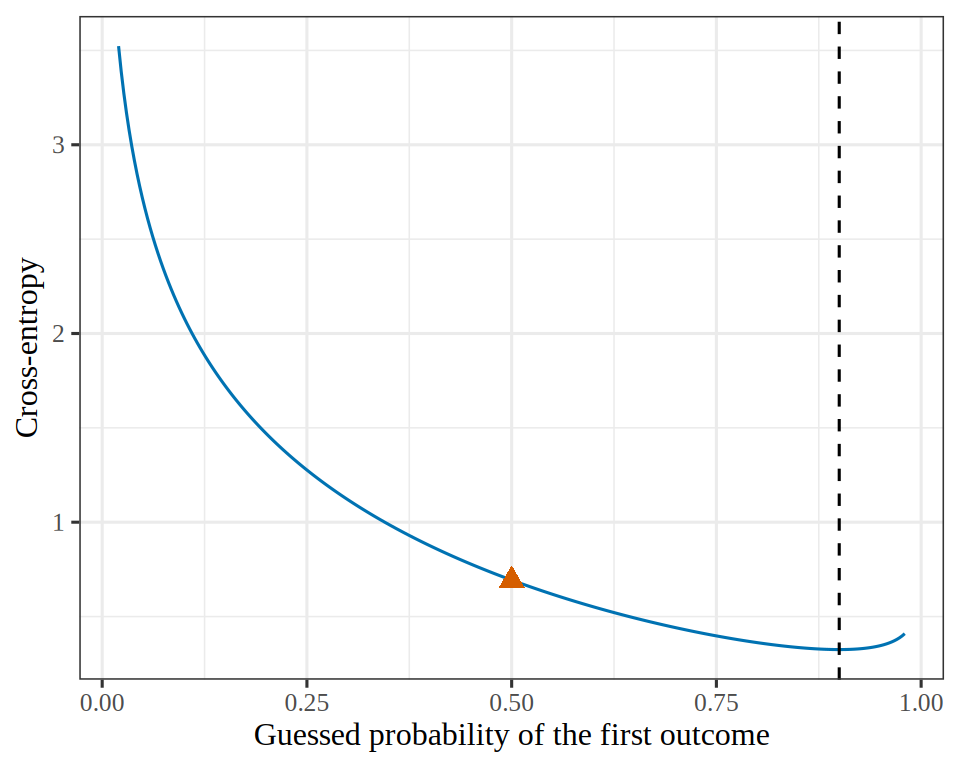
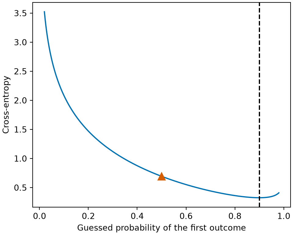
Figure 10: The cross-entropy \(H(\vp, \vq)\) of Example 13 as the guess \(\vq = (q_1, 1 - q_1)\) varies, when the truth is \(\vp = (0.9, 0.1)\). It is lowest where the guess equals the truth (dashed), and the guess \((0.5, 0.5)\) of the example (triangle) lies above that minimum.
(a)
Line plot of the cross-entropy of a two-outcome guess against the guessed probability of the first outcome, for guesses from 0.02 to 0.98, when the true probability of the first outcome is 0.9. The curve falls steeply from the left edge to its lowest point, about 0.33, at a guess of 0.9, marked by a dashed vertical line, then rises slightly toward the right edge. A marked triangle at the guess of 0.5 lies above the minimum.
(b)
Line plot of the cross-entropy of a two-outcome guess against the guessed probability of the first outcome, for guesses from 0.02 to 0.98, when the true probability of the first outcome is 0.9. The curve falls steeply from the left edge to its lowest point, about 0.33, at a guess of 0.9, marked by a dashed vertical line, then rises slightly toward the right edge. A marked triangle at the guess of 0.5 lies above the minimum.

Theorem 6 (The range of the entropy)

Theorem 6 (The range of the entropy) A distribution \(\vp\) over \(M\) outcomes has

\[ 0 \le H(\vp, \vp) \le \log M. \]

The minimum \(0\) holds exactly when one outcome is certain, and the maximum \(\log M\) exactly when \(\vp\) is uniform.

Proof

Proof. By Solution 26 and Solution 27.

Example 14 (Entropy of three distributions over four outcomes)

Example 14 (Entropy of three distributions over four outcomes)  

Show code
en_entropy <- function(p) -sum(ifelse(p > 0, p * log(p), 0))
en_dists <- list(
  certain = c(1, 0, 0, 0),
  skewed = c(0.7, 0.1, 0.1, 0.1),
  uniform = rep(0.25, 4)
)
vapply(en_dists, en_entropy, numeric(1))
 certain   skewed  uniform 
0.000000 0.940448 1.386294 

With \(M = 4\) outcomes, Theorem 6 puts the entropy between \(0\) and \(\log 4 = 1.386\). The certain distribution has entropy \(0\), the uniform distribution has entropy \(\log 4\), and the skewed distribution has entropy 0.94, between the other two.

Figure 11 plots the three cases.

Show code
library(ggplot2)
enf <- do.call(rbind, lapply(names(en_dists), function(nm) {
  data.frame(
    distribution = sprintf("%s (entropy %.2f)", nm, en_entropy(en_dists[[nm]]) + 0),
    outcome = factor(1:4),
    prob = en_dists[[nm]]
  )
}))
enf$distribution <- factor(enf$distribution, levels = unique(enf$distribution))
ggplot(enf, aes(outcome, prob)) +
  geom_col(fill = "#0072B2") +
  facet_wrap(vars(distribution)) +
  labs(x = "Outcome", y = "Probability")
Show code
import matplotlib.pyplot as plt
import numpy as np

def entropy_enf(p):
    p = np.asarray(p, float)
    return -np.sum(np.where(p > 0, p * np.log(np.where(p > 0, p, 1)), 0))

dists_enf = {
    "certain": [1, 0, 0, 0],
    "skewed": [0.7, 0.1, 0.1, 0.1],
    "uniform": [0.25] * 4,
}
fig, axes = plt.subplots(1, 3, figsize=(7, 3.5), sharey=True, layout="constrained")
for ax, (name, p) in zip(axes, dists_enf.items()):
    ax.bar(range(1, 5), p, color="#0072B2");
    ax.set_title(f"{name} (entropy {entropy_enf(p) + 0.0:.2f})", fontsize=9);
    ax.set_xticks(range(1, 5));
    ax.set_xlabel("Outcome");
axes[0].set_ylabel("Probability");
plt.show()
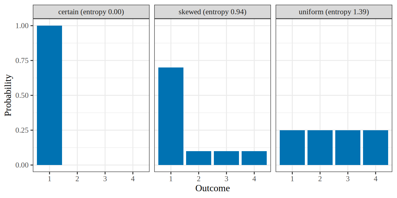
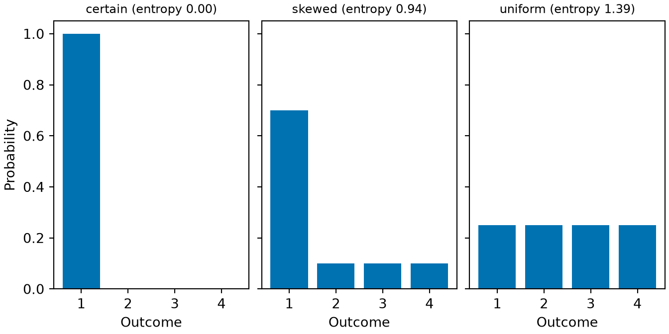
Figure 11: The three distributions of Example 14 put their probability on four outcomes. The entropy rises from \(0\), when one outcome has all of the probability, to \(\log 4\), when the distribution spreads it evenly.
(a)
Three bar charts side by side, each showing a probability distribution over four outcomes. The first, titled certain with entropy 0, has one tall blue bar at 1 for the first outcome and nothing else. The second, titled skewed with entropy 0.94, has a bar of 0.7 for the first outcome and bars of 0.1 for the other three. The third, titled uniform with entropy 1.39, has four equal bars of 0.25.
(b)
Three bar charts side by side, each showing a probability distribution over four outcomes. The first, titled certain with entropy 0, has one tall blue bar at 1 for the first outcome and nothing else. The second, titled skewed with entropy 0.94, has a bar of 0.7 for the first outcome and bars of 0.1 for the other three. The third, titled uniform with entropy 1.39, has four equal bars of 0.25.

2 Cross-entropy as a metric (lower is better)

Definition 5 (Cross-entropy of a classifier)

Definition 5 (Cross-entropy of a classifier) For labels \(\outvar_1, \dots, \outvar_n \in \set{1, \dots, K}\), let \(\vq_i\) be the probability mass function over the \(K\) classes that a classifier gives for observation \(i\), and let \(\vp_i\) be the one that puts probability \(1\) on \(\outvar_i\). The cross-entropy of the classifier in base \(b > 1\) is the sum of its cross-entropy losses, each computed with \(\log_b\) in place of \(\log\),

\[ \crossentropy_b \eqdef \sumin \crossentropyf{\vp_i}{\vq_i}. \tag{1}\]

Lower is better.

Example 15 (The cross-entropy of a logistic regression on the spam emails)

Example 15 (The cross-entropy of a logistic regression on the spam emails) Fit the logistic regression of spam on the percent of words that are “george” and “you” in the spam data of the confusion-matrix exercise. Here \(K = 2\), and the probability \(q_{i \outvar_i}\) that the fit gives to the observed label of email \(i\) is its predicted probability of spam \(\prob_i\) when the email is spam, and \(1 - \prob_i\) otherwise. By Theorem 2, written in base \(2\), the cross-entropy loss of email \(i\) in bits is \(-\log_2 q_{i \outvar_i}\), so the cross-entropy in bits is \(\crossentropy_2 = -\sumin \log_2 q_{i \outvar_i}\).

Show code
spam_data <- readr::read_csv("data/spam-george-you.csv", show_col_types = FALSE)
spam_fit <- glm(spam ~ george + you, family = binomial, data = spam_data)
Warning: glm.fit: fitted probabilities numerically 0 or 1 occurred
Show code
spam_data |>
  dplyr::mutate(
    p_spam = fitted(spam_fit),
    p_true_class = dplyr::if_else(spam == 1, p_spam, 1 - p_spam)
  ) |>
  dplyr::summarize(
    n_emails = dplyr::n(),
    cross_entropy_bits = sum(-log2(p_true_class))
  )

Remark 4 (Units of cross-entropy)

Remark 4 (Units of cross-entropy). The unit of the cross-entropy depends on the base \(b\) of the logarithm:

  • \(b = 2\) gives bits.

  • \(b = e\) gives nats.

  • \(b = 10\) gives hartleys.

Exercise 28 (Reading the cross-entropy sum)

Exercise 28 (Reading the cross-entropy sum) For labels \(\outvar_1, \dots, \outvar_n \in \set{1, \dots, K}\), the cross-entropy of a classifier in base \(b\) is \(\crossentropy_b = \sumin \crossentropyf{\vp_i}{\vq_i}\), where \(p_{ik} = 1\) when \(k = \outvar_i\) and \(p_{ik} = 0\) otherwise. The theorem on the cross-entropy of two mass functions writes each term as a sum over the \(K\) classes:

\[ \crossentropy_b = -\sumin \sumto{k}{K} p_{ik} \log_b q_{ik}. \tag{2}\]

The inner sum runs over all \(K\) classes, but only one of its terms can be nonzero.

Say which term.

Solution 28. Only the term for the observed label can be nonzero. The probability mass function \(\vp_i\) puts probability \(1\) on the observed label \(\outvar_i\), so \(p_{ik} = 0\) for every \(k \ne \outvar_i\). Each of those terms is \(0 \cdot \log_b q_{ik} = 0\), since a term with \(p_{ik} = 0\) is taken to be \(0\) whatever \(q_{ik}\) is.

Exercise 29 (Reading the cross-entropy sum (part 2))

Exercise 29 (Reading the cross-entropy sum (part 2)) Keep \(\vp_i\), \(\vq_i\) and \(\crossentropy_b\) from Exercise 28.

Derive what Equation 2 reduces to once only the term for each observed label is kept.

Solution 29. Only the term for \(k = \outvar_i\) is left, and \(p_{i \outvar_i} = 1\), so

\[ \crossentropy_b = -\sumin \log_b q_{i \outvar_i}. \]

The probabilities that the classifier assigns to the other classes never appear. They matter only because the entries of \(\vq_i\) sum to \(1\), so probability spent on a wrong class is probability taken from the observed one.

Exercise 30 (Reading the cross-entropy sum (part 3))

Exercise 30 (Reading the cross-entropy sum (part 3)) Keep \(\vp_i\), \(\vq_i\) and \(\crossentropy_b\) from Exercise 28.

What is the smallest value \(\crossentropy_b\) can take, and what must the classifier do to reach it?

Solution 30. The smallest value is 0. A probability is at most 1, so \(\log_b q_{i \outvar_i} \le 0\), and each term of the sum in Solution 29 is at least 0. Equality needs \(q_{i \outvar_i} = 1\) for every \(i\): the classifier must put all of its probability on the observed label, every time.

Exercise 31 (Reading the cross-entropy sum (part 4))

Exercise 31 (Reading the cross-entropy sum (part 4)) Keep \(\vp_i\), \(\vq_i\) and \(\crossentropy_b\) from Exercise 28.

What is the largest value \(\crossentropy_b\) can take?

Solution 31. There is no largest value. As \(q_{i \outvar_i} \to 0\), \(-\log_b q_{i \outvar_i} \to \infty\). One confident mistake is enough: a classifier that assigns the observed label a probability of \(10^{-12}\) on a single observation contributes 12 hartleys from that observation alone. This asymmetry is the metric working as intended. A score that only counts mistakes charges 1 for a mistake whether the classifier was hesitant or certain; cross-entropy charges for the certainty.

Exercise 32 (Reading the cross-entropy sum (part 5))

Exercise 32 (Reading the cross-entropy sum (part 5)) Keep \(\vp_i\), \(\vq_i\) and \(\crossentropy_b\) from Exercise 28.

The base \(b\) names the units: 2 gives bits, \(e\) gives nats, 10 gives hartleys. Show that changing \(b\) multiplies \(\crossentropy_b\) by a positive constant, and say what that implies for comparing two classifiers.

Solution 32. The base is a scale factor. By the change-of-base identity, \(\log_b z = \ln z / \ln b\), so

\[ \crossentropy_b = \frac{\crossentropy_e}{\ln b}, \]

and \(\ln b > 0\) for any \(b > 1\). So the three unit choices give three numbers that are positive multiples of each other: 1.386 nats is 2 bits is 0.602 hartleys.

Multiplying every score by the same positive constant leaves their order alone, so a classifier that beats another in bits beats it in nats too, and the base cannot change which model you pick. It changes only the units in which the number is expressed.

Theorem 7 (Cross-entropy of a classifier from the probabilities of the observed labels)

Theorem 7 (Cross-entropy of a classifier from the probabilities of the observed labels) The cross-entropy of a classifier in base \(b\) equals the sum over observations of the negative base-\(b\) logarithm of the probability that the classifier gives to the observed label,

\[ \crossentropy_b = -\sumin \log_b q_{i \outvar_i}. \tag{3}\]

Proof

Proof. Sum Theorem 2, written in base \(b\), over the observations. Solution 29 works the same step from the expanded form in Exercise 28.

Example 16 A classifier with \(K = 3\) classes gives \(\vq_i = (\tfrac12, \tfrac14, \tfrac14)\) for one observation. In bits (\(b = 2\)), Equation 3 gives \(-\log_2 \tfrac12 = 1\) if \(\outvar_i = 1\), and \(-\log_2 \tfrac14 = 2\) if \(\outvar_i\) is \(2\) or \(3\). The probability on the other two classes never enters.

Theorem 8 (Cross-entropy of a classifier is nonnegative)

Theorem 8 (Cross-entropy of a classifier is nonnegative) The cross-entropy of a classifier in base \(b\) is nonnegative,

\[ \crossentropy_b \ge 0, \]

with equality exactly when \(q_{i \outvar_i} = 1\) for every observation \(i\).

Proof

Proof. By Theorem 7, \(\crossentropy_b = -\sumin \log_b q_{i \outvar_i}\). Each \(q_{i \outvar_i}\) is a probability, so \(q_{i \outvar_i} \le 1\), and each term \(-\log_b q_{i \outvar_i}\) is at least \(0\), with equality only when \(q_{i \outvar_i} = 1\). A sum of nonnegative terms is \(0\) exactly when every term is \(0\).

Example 17 (Cross-entropy of two classifiers)

Example 17 (Cross-entropy of two classifiers) On two observations, a classifier assigns the observed labels the probabilities \(0.8\) and \(0.5\). A second classifier assigns them \(1\) and \(1\).

Show code
cn_first <- c(0.8, 0.5)
cn_second <- c(1, 1)
cn_first_terms <- -log2(cn_first)
cn_second_terms <- -log2(cn_second)
cn_first_bits <- sum(cn_first_terms)
cn_second_bits <- sum(cn_second_terms)
cn_bits <- c(first = cn_first_bits, second = cn_second_bits)
cn_bits
   first   second 
1.321928 0.000000 

By Theorem 8 both values are at least \(0\). The first classifier scores 1.322 bits. The second scores exactly \(0\), because it puts all its probability on the observed label every time.

Theorem 9 (Changing the base of cross-entropy rescales it)

Theorem 9 (Changing the base of cross-entropy rescales it) For \(b > 1\), the cross-entropy of a classifier in base \(b\) is its cross-entropy in base \(e\) divided by \(\ln b\),

\[ \crossentropy_b = \frac{\crossentropy_e}{\ln b}. \]

Proof

Proof. The observed-label form is Theorem 7:

\[ \begin{aligned} \crossentropy_b &= -\sumin \log_b q_{i \outvar_i} && \text{(observed-label form)} \\ &= -\sumin \frac{\ln q_{i \outvar_i}}{\ln b} && \text{(change of base, $\log_b z = \ln z / \ln b$)} \\ &= \frac{1}{\ln b} \paren{-\sumin \ln q_{i \outvar_i}} && \text{(factor out the constant $1 / \ln b$)} \\ &= \frac{\crossentropy_e}{\ln b} && \text{(observed-label form in base $e$)}. \end{aligned} \]

Since \(\ln b > 0\), two classifiers are ordered the same way in every base.

Example 18 (One classifier in three units)

Example 18 (One classifier in three units) A classifier assigns the observed labels the probabilities \(0.8\) and \(0.5\) on two observations.

Show code
cb_p <- c(0.8, 0.5)
cb_bits_terms <- -log2(cb_p)
cb_nats_terms <- -log(cb_p)
cb_hartleys_terms <- -log10(cb_p)
cb_bits <- sum(cb_bits_terms)
cb_nats <- sum(cb_nats_terms)
cb_hartleys <- sum(cb_hartleys_terms)
cb_h <- c(bits = cb_bits, nats = cb_nats, hartleys = cb_hartleys)
cb_e <- exp(1)
cb_b <- c(2, cb_e, 10)
cb_ln_b <- log(cb_b)
cb_nats_over_ln_b <- cb_h[["nats"]] / cb_ln_b
names(cb_nats_over_ln_b) <- names(cb_h)
dplyr::bind_rows(
  value = cb_h,
  nats_over_ln_b = cb_nats_over_ln_b,
  .id = "row"
)

The second row is \(\crossentropy_e / \ln b\) for \(b = 2, e, 10\), and by Theorem 9 it matches the first row. Every classifier’s score is multiplied by the same \(1/\ln b\), so the ordering of classifiers does not change with the base.

Other names for cross-entropy, and two conventions to state

Software and statistics each renamed this quantity. Log loss and logistic loss are the same number, and so is the negative log-likelihood of the labels under the model, since Theorem 2 gives each loss as \(-\log q_{i \outvar_i}\), the log-likelihood of label \(\outvar_i\) with its sign reversed. Generalized linear models add deviance, which for one label per observation is twice the summed negative log-likelihood.

Settle two conventions before comparing one of these numbers with another source’s. The notation choices page explains both.

Which base. The definition of \(\crossentropy_b\) leaves the base \(b\) free. Theorem 9 shows the base cannot change which of two classifiers you would pick, but it does change the number itself, so state the base whenever you quote one.

Summed or averaged. The cross-entropy of a classifier \(\crossentropy_b\) sums over all \(n\) observations. Most software reports the mean, \(\avgcrossent_b = \crossentropy_b / n\), under the same name, as Remark 1 says of the log loss. The perplexity is defined from the mean, not from the sum.

Read

GeeksforGeeks explains the cross-entropy loss [3].

3 Tracing the origin of cross-entropy

Cross-entropy comes from Claude Shannon’s 1948 theory of communication [4], where it measures the average number of bits per symbol needed to encode a source with a code designed for another distribution.

A code designed for the source itself needs no more bits per symbol than a code designed for another distribution. The difference is the Kullback–Leibler divergence. The difference is zero only when the code’s distribution equals the source’s. The coding theorems behind these statements are in Source Coding in Information Theory for Data Science.

Minimizing cross-entropy over \(\vq\) moves \(\vq\) toward \(\vp\), and fitting a logistic regression minimizes the sum of these cross-entropies over the observations, with one \(\vq\) for each observation and all of them determined by the shared \(\vcoef\). The reference distribution \(\vp\) puts probability \(1\) on the observed label and \(0\) on the other outcome, and the model’s distribution \(\vq\) is \((1 - \prob, \prob)\). A distribution that puts probability \(1\) on a single outcome has entropy \(0\), so for a labeled training point the cross-entropy equals the Kullback–Leibler divergence.

The base of the logarithm sets the unit of information. Base \(2\) measures information in bits, and the natural logarithm measures it in nats. Because \(\log_2 z = \ln z / \ln 2\), switching between them multiplies every term by a positive constant, so it does not change the minimizer. In this chapter, \(\log\) is the natural logarithm, so the losses are measured in nats.

Watch

Read

GeeksforGeeks explains binary cross-entropy [9].

4 The gradient

In general there is no closed-form expression for \(\hvcoef\), so it is computed iteratively by the methods of the gradient descent chapter. Those methods need the gradient of the total log loss. Exercise 33 shows that the derivative of the logistic function cancels in this gradient, leaving an expression of the same form as the least-squares gradient of linear regression. Later in this section, Figure 18 draws the total log loss on the WCGS data as a bowl over two slopes, with its gradient entries crossing zero at the bottom of the bowl and its Hessian entries measuring how steep the bowl is.

Exercise 33 (The gradient, and the factor that cancels)

Exercise 33 (The gradient, and the factor that cancels) Let \(z_i = \dprod{\vcoef}{\vx_i}\), which is the log-odds of \(\prob_i = \sigmoid(z_i)\). Let \(C_i = -\llik_i\) be observation \(i\)’s contribution to the total log loss of Exercise 3, where \(\llik_i\) is the log-likelihood contribution of one binary outcome in terms of the log-odds: \(\llik_i = \outvar_i z_i + \log(1 - \prob_i)\).

Show that \(\dfrac{\partial C_i}{\partial z_i} = \prob_i - \outvar_i\), using \(\sigmoid' = \sigmoid(1-\sigmoid)\) from part 3 of the sigmoid properties exercise and without splitting into cases.

Solution 33. Write \(\sigmoid'(z_i)\) for the derivative of \(\sigmoid\) at \(z_i\). Then

\[ \begin{aligned} \frac{\partial C_i}{\partial z_i} &= -\frac{\partial}{\partial z_i}\paren{\outvar_i z_i + \log\paren{1 - \sigmoid(z_i)}} && \text{(}C_i = -\llik_i\text{)} \\ &= -\outvar_i - \frac{\partial}{\partial z_i}\log\paren{1 - \sigmoid(z_i)} && \text{(derivative of a sum, and of } \outvar_i z_i\text{)} \\ &= -\outvar_i + \frac{\sigmoid'(z_i)}{1 - \sigmoid(z_i)} && \text{(chain rule)} \\ &= -\outvar_i + \frac{\sigmoid(z_i)\paren{1 - \sigmoid(z_i)}}{1 - \sigmoid(z_i)} && \text{(}\sigmoid' = \sigmoid(1 - \sigmoid)\text{)} \\ &= -\outvar_i + \sigmoid(z_i) && \text{(cancel } 1 - \sigmoid(z_i)\text{)} \\ &= \prob_i - \outvar_i && \text{(}\prob_i = \sigmoid(z_i)\text{)}. \end{aligned} \]

In terms of the log-odds \(z_i\), the label \(\outvar_i\) appears only in the term \(\outvar_i z_i\), which is linear in \(z_i\). That term differentiates to \(\outvar_i\) with no case split.

The derivative of the cost with respect to the log-odds is the predicted probability minus the observed label. It contains no exponential and no factor of \(\sigmoid'\).

Exercise 34 (The gradient, and the factor that cancels (part 2))

Exercise 34 (The gradient, and the factor that cancels (part 2)) Use the setup of Exercise 33.

Hence give \(\grad_{\vcoef} C\) for the whole dataset, first as a sum over observations and then in matrix form, where \(\design(\mx)\) is the \(\nobs \times (\ninputvars+1)\) design matrix and \(\vprob\) is the vector of fitted probabilities.

Solution 34. Because \(z_i = \dprod{\vcoef}{\vx_i}\), the gradient \(\grad_{\vcoef} z_i\) is \(\vx_i\). Then

\[ \begin{aligned} \grad_{\vcoef} C &= \sumin \grad_{\vcoef} C_i && \text{(gradient of a sum)} \\ &= \sumin \frac{\partial C_i}{\partial z_i}\,\grad_{\vcoef} z_i && \text{(chain rule)} \\ &= \sumin \paren{\prob_i - y_i}\,\grad_{\vcoef} z_i && \text{(}\partial C_i / \partial z_i = \prob_i - y_i\text{)} \\ &= \sumin \paren{\prob_i - y_i}\vx_i && \text{(}\grad_{\vcoef} z_i = \vx_i\text{)} \\ &= \tp{\design(\mx)}\paren{\vprob - \vy} && \text{(row } i \text{ of } \design(\mx) \text{ is } \tp{\vx_i}\text{)}. \end{aligned} \]

Least squares has gradient \(\tp{\design(\mx)}\paren{\design(\mx)\vcoef - \vy}\), up to a constant factor, which is the same expression with the fitted values \(\design(\mx)\vcoef\) of least squares in place of \(\vprob\). Both gradients are the transposed design matrix times a vector of fitted values minus labels. Only the map from \(\vcoef\) to the fitted values differs, and because \(\vprob\) is a nonlinear function of \(\vcoef\), setting the logistic gradient to zero gives equations with no closed-form solution in general (the gradient descent chapter’s exercise on why there is no closed form).

One observation at a time, the factor \(\prob_i - y_i\) shows what each observation does to a descent step \(\vcoef \leftarrow \vcoef - \learnrate\,\grad_{\vcoef} C\):

  • If \(y_i = 0\) and \(\prob_i \approx 0\), or \(y_i = 1\) and \(\prob_i \approx 1\), then \(\prob_i - y_i\) is near zero, and the observation changes the gradient very little.
  • If \(y_i = 1\) and \(\prob_i \approx 0\), the observation’s term in the step adds about \(\learnrate\,\vx_i\) to \(\vcoef\). That term raises the log-odds \(\dprod{\vcoef}{\vx_i}\) by about \(\learnrate\norm{\vx_i}^2\), and so raises \(\prob_i\) toward \(1\).
  • If \(y_i = 0\) and \(\prob_i \approx 1\), the observation’s term subtracts about \(\learnrate\,\vx_i\) from \(\vcoef\), which lowers the log-odds and so lowers \(\prob_i\) toward \(0\).

The absolute value \(\abs{\prob_i - \outvar_i}\) is the probability that the model gives to the label \(1 - \outvar_i\), which the observation does not have. Each observation therefore contributes to the gradient in the direction of its feature vector \(\vx_i\), weighted by the probability that the model gives to the wrong label.

Exercise 35 (The gradient, and the factor that cancels (part 3))

Exercise 35 (The gradient, and the factor that cancels (part 3)) Use the setup of Exercise 33.

In Exercise 33, the factor \(\sigmoid'(z_i)\) cancels. Differentiate the squared-error cost \(S_i = \tfrac{1}{2}\paren{\prob_i - \outvar_i}^2\) with respect to \(z_i\) instead.

Solution 35. By the chain rule,

\[ \begin{aligned} \frac{\partial S_i}{\partial z_i} &= \paren{\prob_i - y_i}\sigmoid'(z_i) && \text{(chain rule)} \\ &= \paren{\prob_i - y_i}\prob_i\paren{1 - \prob_i} && \text{(}\sigmoid' = \sigmoid(1 - \sigmoid)\text{)}. \end{aligned} \]

The factor \(\sigmoid'(z_i)\) stays in this derivative, because squared error has no logarithm whose derivative cancels it.

Exercise 36 (The gradient, and the factor that cancels (part 3b))

Exercise 36 (The gradient, and the factor that cancels (part 3b)) Use the setup of Exercise 33.

Compare the derivative of Exercise 33 with the derivative of Exercise 35 at \(z_i = 8\) with \(\outvar_i = 0\), an observation whose predicted probability is close to \(1\) while its observed label is \(0\).

Solution 36. This continues Solution 35.

At \(z_i = 8\) with \(y_i = 0\), the predicted probability \(\prob_i = \sigmoid(8)\) is 0.99966, so

  • the log loss has derivative \(\prob_i - \outvar_i\), which is 0.99966;
  • squared error has derivative \(\prob_i \cdot \prob_i\paren{1 - \prob_i}\), which is 0.0003351.

Exercise 37 (The gradient, and the factor that cancels (part 3c))

Exercise 37 (The gradient, and the factor that cancels (part 3c)) Use the setup of Exercise 33.

Report the ratio of the derivative of Exercise 33 to the derivative of Exercise 35 at \(z_i = 8\) with \(\outvar_i = 0\).

Solution 37. This continues Solution 36.

At \(z_i = 8\) with \(y_i = 0\), the log-loss derivative of Solution 36 is about 2983 times the squared-error derivative of Solution 36, and the ratio \(1 / \paren{\prob_i(1 - \prob_i)}\) grows without bound as \(\abs{z_i}\) increases.

The model gives probability 0.9997 to the wrong class, yet squared error gives a gradient of only 0.000335, so gradient descent on squared error changes \(\vcoef\) very little on this observation. In Solution 33, the factor \(1/(1 - \prob_i)\) from differentiating the logarithm cancels \(\sigmoid'(z_i)\) (here \(y_i = 0\); for \(y_i = 1\) the factor is \(1/\prob_i\)), so the log loss has no such factor.

The solution to part 4c of the sigmoid properties exercise showed that \(\sigmoid\) is nearly constant far from the decision boundary. Under the log loss, that flatness does not shrink the gradient on misclassified observations.

Exercise 38 (The gradient, and the factor that cancels (part 4))

Exercise 38 (The gradient, and the factor that cancels (part 4)) Use the setup of Exercise 33.

Show that \(\norm{\grad_{\vcoef} C_i} < \norm{\vx_i}\) for every \(\vcoef\).

Solution 38. Because \(\grad_{\vcoef} C_i = (\prob_i - y_i)\vx_i\),

\[ \norm{\grad_{\vcoef} C_i} = \abs{\prob_i - y_i} \cdot \norm{\vx_i}. \]

By part 1b of the sigmoid properties exercise, \(\prob_i \in (0,1)\), and \(\outvar_i \in \{0,1\}\), so \(\abs{\prob_i - \outvar_i} < 1\), and the bound follows.

Exercise 39 (The gradient, and the factor that cancels (part 4b))

Exercise 39 (The gradient, and the factor that cancels (part 4b)) Use the setup of Exercise 33.

Explain what the bound of Exercise 38 guarantees.

Solution 39. This continues Solution 38.

Solution 38 guarantees that no single observation can give a gradient larger in norm than \(\norm{\vx_i}\), however wrong the predicted probability is. The contribution of an observation to a gradient step is bounded by the norm of its feature vector, which is one reason to standardize features that are on different scales before fitting.

Exercise 40 (The gradient, and the factor that cancels (part 5))

Exercise 40 (The gradient, and the factor that cancels (part 5)) Use the setup of Exercise 33.

At a minimizer of \(C\), the gradient equals the zero vector, which gives the score equations \(\tp{\design(\mx)}(\vprob - \vy) = \vzero\). Suppose the first column of \(\design(\mx)\) is a column of ones, and the second is a binary indicator \(\predvar_{i} \in \{0, 1\}\) of membership in a group. State in words what each of those two equations implies about the fitted model.

Solution 40. The column of ones gives \(\sum_i \prob_i = \sum_i \outvar_i\): the sum of the fitted probabilities equals the observed number of positive outcomes. For example, if \(30\) of \(100\) training observations have \(y_i = 1\), the fitted probabilities sum to \(30\). A logistic regression with an intercept therefore predicts the right number of positive outcomes on the training set as a whole, which is called being calibrated in aggregate.

The binary indicator gives \(\sum_{i \,:\, x_i = 1} \prob_i = \sum_{i \,:\, x_i = 1} y_i\), so the same equality holds within the group where \(x_i = 1\). Subtracting this equation from the intercept equation shows that it also holds in the complementary group, where \(x_i = 0\).

Each indicator feature therefore makes the fit calibrated in aggregate within the group it defines. A categorical predictor coded with indicator variables, together with an intercept, makes the fitted probabilities sum to the observed number of positive outcomes in every level of the predictor. The score equations impose no condition on groups defined by variables that are not in the design matrix, and the fit can be miscalibrated on those groups.

Exercise 41 (Leaving the intercept unpenalized)

Exercise 41 (Leaving the intercept unpenalized) Use the setup of Exercise 33.

\(\lpnorm{2}\) regularization replaces the empirical risk \(\emprisk\) by \(\emprisk + \regpar\sumto{k}{\ninputvars}\coef{k}^2\), summing from \(k = 1\) so that the intercept \(\coef{0}\) is not penalized. Determine how penalizing \(\coef{0}\) would change the intercept score equation of Exercise 40.

Solution 41. The intercept column of \(\design(\mx)\) is a column of ones, so by Solution 34 the derivative of \(\emprisk = \tfrac1n C\) with respect to \(\coef{0}\) is

\[ \frac{\partial \emprisk}{\partial\coef{0}} = \frac1n\sum_i\paren{\prob_i - y_i}. \]

Without a penalty on \(\coef{0}\), setting this derivative to zero gives the intercept score equation of Exercise 40, \(\sum_i \prob_i = \sum_i y_i\): the fitted probabilities sum to the observed number of positive outcomes.

Now add \(\regpar\coef{0}^2\) to the objective. At the minimizer, the derivative with respect to \(\coef{0}\) is zero:

\[ \begin{aligned} \frac1n\sum_i\paren{\prob_i - y_i} + 2\regpar\hcoef{0} &= 0 && \text{(derivative of the penalized objective)} \\ \frac1n\sum_i\paren{\prob_i - y_i} &= -2\regpar\hcoef{0} && \text{(subtract } 2\regpar\hcoef{0}\text{)} \\ \sum_i\paren{\prob_i - y_i} &= -2n\regpar\hcoef{0} && \text{(multiply by } n\text{)} \\ \sum_i \prob_i - \sum_i y_i &= -2n\regpar\hcoef{0} && \text{(split the sum)} \\ \sum_i \prob_i &= \sum_i y_i - 2n\regpar\hcoef{0} && \text{(add } \textstyle\sum_i y_i\text{)}. \end{aligned} \]

The fitted probabilities no longer sum to the observed count: their sum is too small when \(\hcoef{0} > 0\) and too large when \(\hcoef{0} < 0\).

Exercise 42 (Leaving the intercept unpenalized (part 10b))

Exercise 42 (Leaving the intercept unpenalized (part 10b)) Use the setup of Exercise 33.

Use the result of Exercise 41 to explain why \(\coef{0}\) is left unpenalized.

Solution 42. This continues Solution 41.

Penalizing \(\coef{0}\) moves the fitted probabilities away from the observed count (Solution 41). When the features are centered, \(\coef{0}\) is the log-odds that the model gives an observation with average features, which is usually negative for an outcome with prevalence below \(\tfrac12\). Shrinking \(\coef{0}\) toward \(0\) then moves the average predicted probability toward \(\tfrac12\), so a rare outcome is predicted too often and a common outcome too rarely.

A second reason is that a penalty on \(\coef{0}\) makes the fit depend on where the features’ origin is. A penalty on a slope \(\coef{k}\) penalizes a large rate of change of the log-odds with respect to \(x_k\), but the intercept is not a rate of change. Without a penalty on \(\coef{0}\), centering a feature, \(x_k \mapsto x_k - \bar x_k\), changes \(\hcoef{0}\) and leaves every slope and every fitted probability unchanged. With a penalty on \(\coef{0}\), the penalty depends on the size of \(\coef{0}\), so the fitted probabilities depend on the choice of origin for the features.

Definition 6 (Residual of a logistic regression)

Definition 6 (Residual of a logistic regression) The residual of observation \(i\) in logistic regression is its predicted probability minus its label,

\[ \prob_i - \outvar_i, \qquad \prob_i = \sigmoidf{\dprod{\vcoef}{\vpredvar_i}}. \]

It is the negative of the response residual \(\outvar_i - \prob_i\), and it is in \((-1, 1)\).

Example 19 (Residuals of two men in the WCGS data)

Example 19 (Residuals of two men in the WCGS data) In the model of the logistic function example, the first man in data/wcgs.csv with coronary heart disease has \(\outvar_i = 1\) and fitted probability \(\prob_i = 0.069\), so his residual \(\prob_i - \outvar_i\) is -0.931. The first man without it has \(\outvar_i = 0\) and \(\prob_i = 0.134\), so his residual is \(0.134\).

Figure 12 draws one vertical segment for each man.

Show code
library(ggplot2)
ggplot(lrv_pts) +
  aes(x = man, colour = man) +
  geom_segment(
    aes(xend = man, y = label, yend = prob, linetype = man),
    linewidth = 1
  ) +
  geom_point(aes(y = label, shape = man), size = 3) +
  geom_point(aes(y = prob), shape = 4, size = 3) +
  scale_colour_manual(values = c("#0072B2", "#D55E00")) +
  scale_shape_manual(values = c(16, 17)) +
  scale_linetype_manual(values = c("solid", "dashed")) +
  scale_y_continuous(limits = c(0, 1)) +
  labs(x = NULL, y = "Label (point) and fitted probability (cross)") +
  theme(legend.position = "none")
Show code
import matplotlib.pyplot as plt

pts_lrv = r.lrv_pts
fig, ax = plt.subplots(figsize=(6, 4), layout="constrained")
for i, (colour, marker, style) in enumerate([("#0072B2", "o", "-"), ("#D55E00", "^", "--")]):
    ax.vlines(i, pts_lrv["label"][i], pts_lrv["prob"][i], color=colour, linestyle=style, linewidth=2);
    ax.plot(i, pts_lrv["label"][i], color=colour, marker=marker, markersize=8, linestyle="");
    ax.plot(i, pts_lrv["prob"][i], color=colour, marker="x", markersize=8, linestyle="");
ax.set_xticks([0, 1], ["first man with CHD", "first man without CHD"]);
ax.set_xlim(-0.5, 1.5);
ax.set_ylim(-0.05, 1.05);
ax.set_ylabel("Label (point) and fitted probability (cross)");
plt.show()
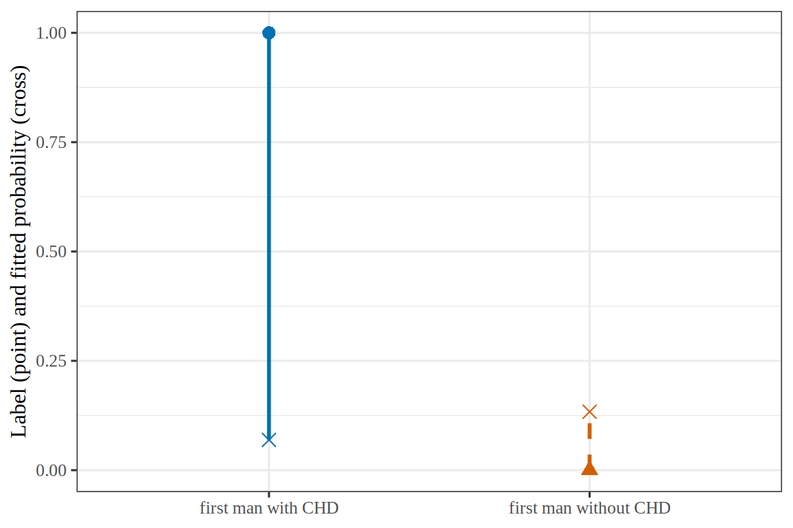
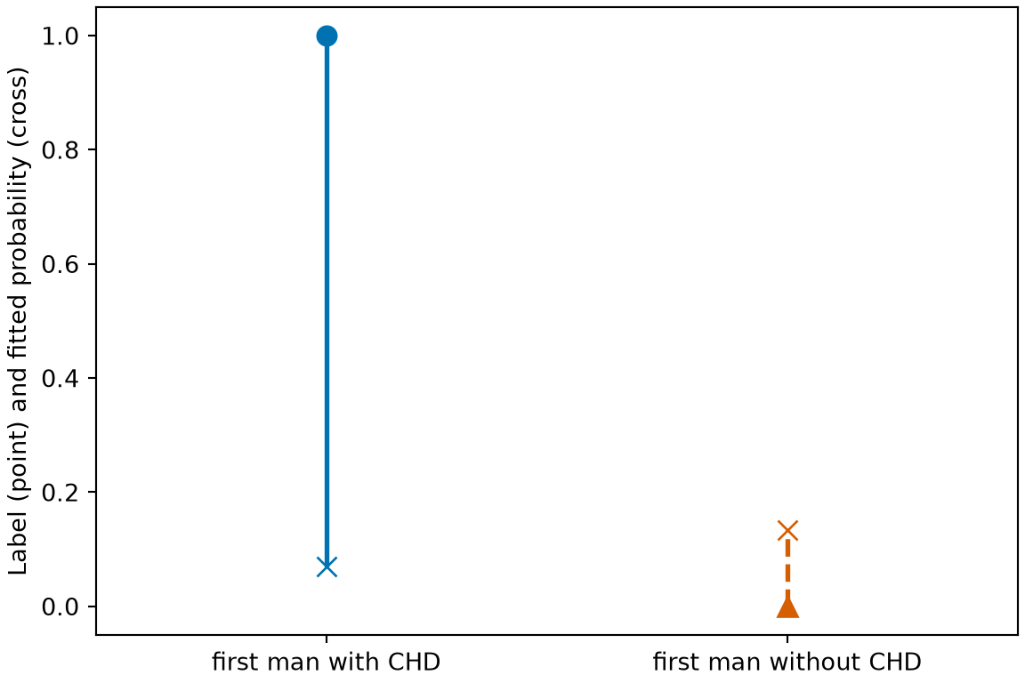
Figure 12: The two men of Example 19, with each man’s label and the probability that the model gives to a label of \(1\). The vertical distance between them is the size of his residual.
(a)
Plot of two men from the WCGS data. For the first man with coronary heart disease, a blue circle at his label 1 is joined by a solid vertical segment to a cross at his fitted probability, 0.069. For the first man without it, a vermilion triangle at his label 0 is joined by a dashed vertical segment to a cross at his fitted probability, 0.134. The segment for the man with the disease is much longer.
(b)
lrv_alt

Theorem 10 (Derivative of the log loss with respect to the log-odds)

Theorem 10 (Derivative of the log loss with respect to the log-odds) Let \(z_i = \dprod{\vcoef}{\vpredvar_i}\) and \(\prob_i = \sigmoidf{z_i}\). The log loss \(C_i\) of observation \(i\) has derivative

\[ \derivf{C_i}{z_i} = \prob_i - \outvar_i, \]

the residual of Definition 6.

Proof

Proof. By Solution 33.

Example 20 (The residual of a man with a body mass index of 25)

Example 20 (The residual of a man with a body mass index of 25) In the model of the logistic function example, the man with \(\text{bmi} = 25\) of the logistic symmetry example has \(\prob_i = 0.083\). If he has coronary heart disease, then \(\outvar_i = 1\), and \(\derivf{C_i}{z_i} = \prob_i - 1\), which is -0.917. If he does not, then \(\outvar_i = 0\), and the derivative is \(\prob_i\), which is 0.083. The derivative is about 11 times as large in magnitude when the label is \(1\), because the model gives his disease a low probability.

Figure 13 plots the derivative under each of the two cases.

Show code
library(ggplot2)
ggplot(lrf_bars) +
  aes(label, derivative, fill = label, linetype = label) +
  geom_hline(yintercept = 0, colour = "grey40") +
  geom_col(colour = "black", width = 0.6) +
  scale_fill_manual(values = c("label 1" = "#0072B2", "label 0" = "#D55E00")) +
  scale_linetype_manual(values = c("label 1" = "solid", "label 0" = "dashed")) +
  labs(x = NULL, y = "Derivative of the loss", fill = NULL, linetype = NULL)
Show code
import matplotlib.pyplot as plt

deriv_lrf = r.lr25_deriv
fig, ax = plt.subplots(figsize=(6, 4), layout="constrained")
ax.axhline(0, color="grey");
ax.bar(["label 1"], [deriv_lrf[0]], color="#0072B2", edgecolor="black", width=0.6);
ax.bar(["label 0"], [deriv_lrf[1]], color="#D55E00", edgecolor="black", linestyle="--", width=0.6);
ax.set_ylabel("Derivative of the loss");
plt.show()
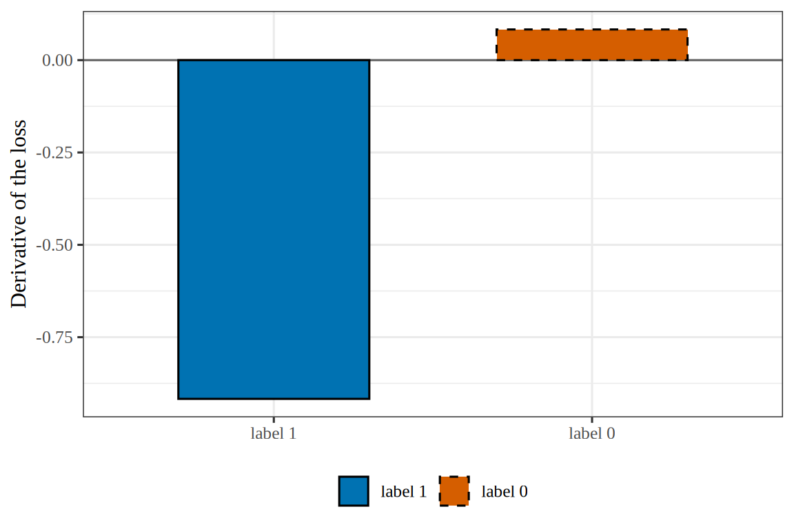
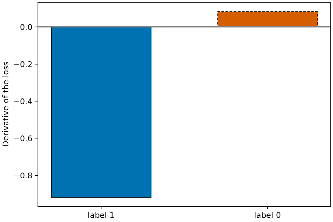
Figure 13: The derivative of the loss with respect to the log-odds for the man of Example 20, under each of the two labels. The label \(1\) is much farther from the probability that the model gives him, so its derivative is much larger in magnitude.
(a)
Bar chart of the derivative of the loss with respect to the log-odds for the man with a body mass index of 25, under each of the two labels. The blue bar for the label 1 extends down to -0.917. The vermilion bar with a dashed outline for the label 0 extends up to 0.083. A solid grey horizontal line marks 0.
(b)
lrf_alt

Theorem 11 (Gradient of the total log loss)

Theorem 11 (Gradient of the total log loss) The gradient of the total log loss with respect to \(\vcoef\) is

\[ \begin{aligned} \grad C(\vcoef) &= \sumin \paren{\prob_i - \outvar_i} \vpredvar_i \\ &= \tp{\design} \paren{\vprob - \voutvar}, \end{aligned} \]

where \(\design\) is the design matrix, with the column of ones that holds the intercept, and \(\vprob\) is the vector of fitted probabilities.

Proof

Proof. By Theorem 10 and the chain rule, as in Solution 34.

Example 21 (The gradient at zero coefficients)

Example 21 (The gradient at zero coefficients) Consider six points with predictor values \(1, \dots, 6\) and labels \(0, 0, 1, 0, 1, 1\), at \(\vcoef = \vzero\). Every fitted probability is then \(\prob_i = \sigmoidf{0}\), which is \(1/2\). The intercept entry of \(\tp{\design} \paren{\vprob - \voutvar}\) is \(\sumin \paren{1/2 - \outvar_i}\), which is 0. The slope entry is \(\sumin \paren{1/2 - \outvar_i} \predvar_i\), which is -3.5. Because the slope entry is negative, the loss decreases as the slope increases from \(0\), so a first step of gradient descent increases the slope.

Figure 14 draws one vertical segment for each of the six points.

Show code
library(ggplot2)
lgg_pts <- data.frame(
  x = 1:6,
  label = factor(c(0, 0, 1, 0, 1, 1), levels = c(1, 0))
)
ggplot(lgg_pts, aes(x, as.numeric(as.character(label)), colour = label)) +
  geom_hline(yintercept = 0.5, linetype = "dashed", colour = "grey50") +
  geom_segment(
    aes(xend = x, yend = 0.5, linetype = label), linewidth = 1
  ) +
  geom_point(aes(shape = label), size = 3) +
  scale_colour_manual(values = c("1" = "#0072B2", "0" = "#D55E00")) +
  scale_shape_manual(values = c("1" = 16, "0" = 17)) +
  scale_linetype_manual(values = c("1" = "solid", "0" = "dashed")) +
  scale_x_continuous(breaks = 1:6) +
  labs(x = "Predictor", y = "Label", colour = "Label", shape = "Label", linetype = "Label")
Show code
import matplotlib.pyplot as plt
import numpy as np

x_lgg = np.arange(1, 7)
y_lgg = np.array([0, 0, 1, 0, 1, 1])
fig, ax = plt.subplots(figsize=(6, 4), layout="constrained")
ax.axhline(0.5, color="grey", linestyle="--");
for label_lgg, colour, marker, style in [(1, "#0072B2", "o", "-"), (0, "#D55E00", "^", "--")]:
    keep_lgg = y_lgg == label_lgg
    ax.vlines(x_lgg[keep_lgg], 0.5, y_lgg[keep_lgg], color=colour, linestyle=style, linewidth=2);
    ax.plot(x_lgg[keep_lgg], y_lgg[keep_lgg], color=colour, marker=marker, markersize=8,
            linestyle="", label=f"label {label_lgg}");
ax.set_xticks(x_lgg);
ax.set_xlabel("Predictor");
ax.set_ylabel("Label");
fig.legend(loc="outside lower center", ncol=2);
plt.show()
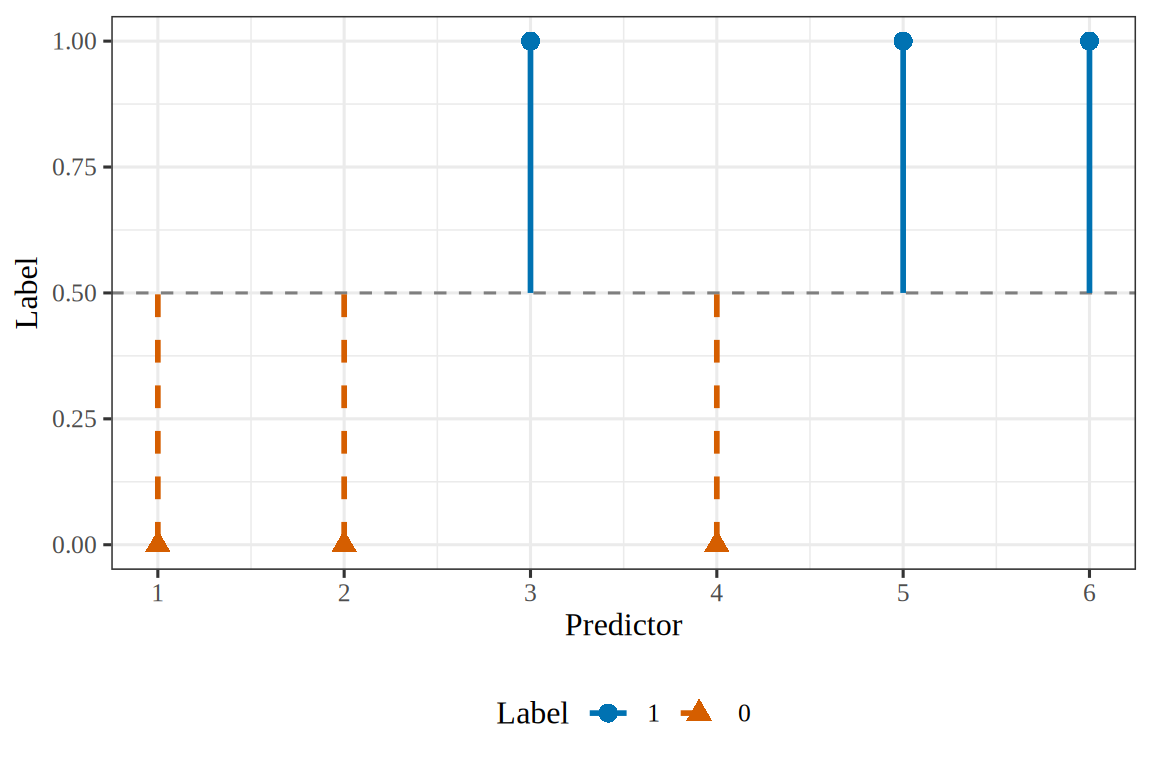
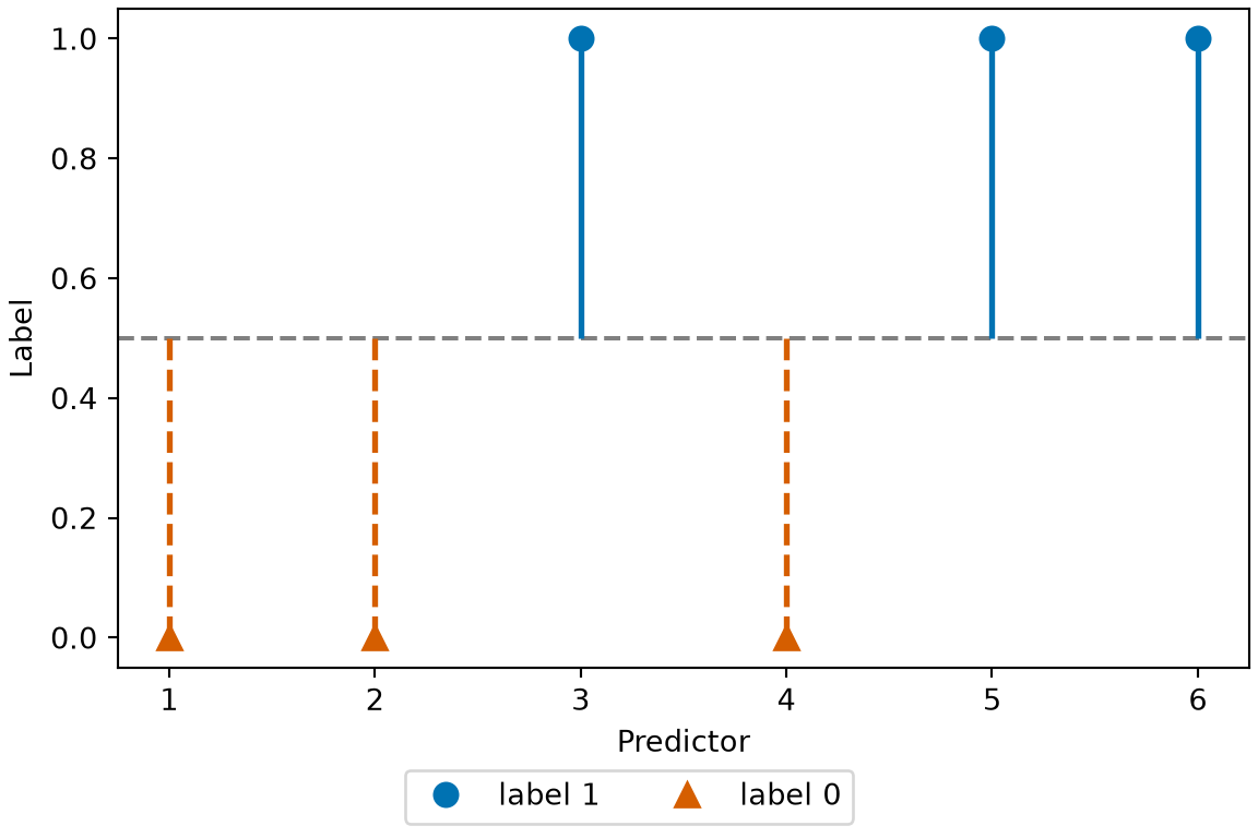
Figure 14: The six points of Example 21, with the fitted probability \(1/2\) that they all have at zero coefficients (dashed line). Each vertical segment is the distance between a point’s label and that probability, which is the size of its residual.
(a)
Plot of the label of six points against their predictor value, 1 to 6, with a dashed grey horizontal line at 0.5, the fitted probability at zero coefficients. Blue circles at the label 1 mark the points at 3, 5 and 6, and vermilion triangles at the label 0 mark the points at 1, 2 and 4. A vertical segment joins each point to the line at 0.5, each of length 0.5. The segments of the three points at the label 1 are solid and the segments of the three points at the label 0 are dashed.
(b)
Plot of the label of six points against their predictor value, 1 to 6, with a dashed grey horizontal line at 0.5, the fitted probability at zero coefficients. Blue circles at the label 1 mark the points at 3, 5 and 6, and vermilion triangles at the label 0 mark the points at 1, 2 and 4. A vertical segment joins each point to the line at 0.5, each of length 0.5. The segments of the three points at the label 1 are solid and the segments of the three points at the label 0 are dashed.

Theorem 12 (Hessian of the total log loss)

Theorem 12 (Hessian of the total log loss) The Hessian of the total log loss with respect to \(\vcoef\) is

\[ \begin{aligned} \grad^2 C(\vcoef) &= \sumin \prob_i \paren{1 - \prob_i} \vpredvar_i \tp{\vpredvar_i} \\ &= \tp{\design} W \design, \end{aligned} \]

where \(W\) is the diagonal matrix with entries \(\prob_i \paren{1 - \prob_i}\). Because each \(\prob_i \paren{1 - \prob_i} > 0\), \(\tp{\design} W \design\) is positive semidefinite for every \(\vcoef\), so \(C(\vcoef)\) is convex and therefore a friendly loss.

Proof

Proof. By Theorem 11, \(\grad C(\vcoef) = \sumin \paren{\prob_i - \outvar_i} \vpredvar_i\). Only \(\prob_i\) depends on \(\vcoef\), and by the logistic derivative theorem and the chain rule the gradient of \(\prob_i\) is \(\grad \prob_i = \prob_i \paren{1 - \prob_i} \vpredvar_i\). Differentiating each term of the sum gives \(\prob_i \paren{1 - \prob_i} \vpredvar_i \tp{\vpredvar_i}\), and the sum of these is \(\tp{\design} W \design\).

Example 22 (The Hessian at zero coefficients)

Example 22 (The Hessian at zero coefficients) For the six points of Example 21 at \(\vcoef = \vzero\), every \(\prob_i = 1/2\), so \(W = \tfrac14 I\).

# the six points, with the column of ones for the intercept
x_six <- 1:6
design_six <- cbind(1, x_six)
# fitted probabilities at zero coefficients, and their weights p (1 - p)
p_zero <- rep(1 / 2, 6)
w_zero <- p_zero * (1 - p_zero)
# the Hessian: design' W design
crossprod(design_six, w_zero * design_six)
           x_six
      1.50  5.25
x_six 5.25 22.75
import numpy as np

# the six points, with the column of ones for the intercept
x_six = np.arange(1, 7)
design_six = np.column_stack([np.ones(6), x_six])
# fitted probabilities at zero coefficients, and their weights p (1 - p)
p_zero = np.full(6, 0.5)
w_zero = p_zero * (1 - p_zero)
# the Hessian: design' W design
print(design_six.T @ (w_zero[:, None] * design_six))
[[ 1.5   5.25]
 [ 5.25 22.75]]

The intercept entry is \(\tfrac14 \cdot 6\), which is 1.5. The off-diagonal entry is \(\tfrac14 \sum_i \predvar_i\), which is 5.25. The slope entry is \(\tfrac14 \sum_i \predvar_i^2\), which is 22.75.

Figure 15 displays the entries.

Show code
library(ggplot2)
hsf_x <- 1:6
hsf_design <- cbind(1, hsf_x)
hsf_h <- crossprod(hsf_design, (1 / 4) * hsf_design)
hsf_cells <- expand.grid(row = c("intercept", "slope"), col = c("intercept", "slope"))
hsf_cells$value <- as.vector(hsf_h)
ggplot(hsf_cells, aes(col, row, fill = value)) +
  geom_tile(colour = "white") +
  geom_text(aes(label = value), colour = "black", size = 5) +
  scale_fill_gradient(low = "#F0E442", high = "#56B4E9") +
  scale_y_discrete(limits = c("slope", "intercept")) +
  labs(x = "Column", y = "Row", fill = "Entry")
Show code
import matplotlib.pyplot as plt
from matplotlib.colors import LinearSegmentedColormap
import numpy as np

x_hsf = np.arange(1, 7)
design_hsf = np.column_stack([np.ones(6), x_hsf])
h_hsf = design_hsf.T @ (0.25 * design_hsf)
fig, ax = plt.subplots(figsize=(6, 4), layout="constrained")
im = ax.imshow(h_hsf, cmap=LinearSegmentedColormap.from_list("hsf", ["#F0E442", "#56B4E9"]))
for i in range(2):
    for j in range(2):
        ax.text(j, i, f"{h_hsf[i, j]:g}", ha="center", va="center", fontsize=14);
ax.set_xticks([0, 1], ["intercept", "slope"]);
ax.set_yticks([0, 1], ["intercept", "slope"]);
ax.set_xlabel("Column");
ax.set_ylabel("Row");
fig.colorbar(im, ax=ax, label="Entry");
plt.show()
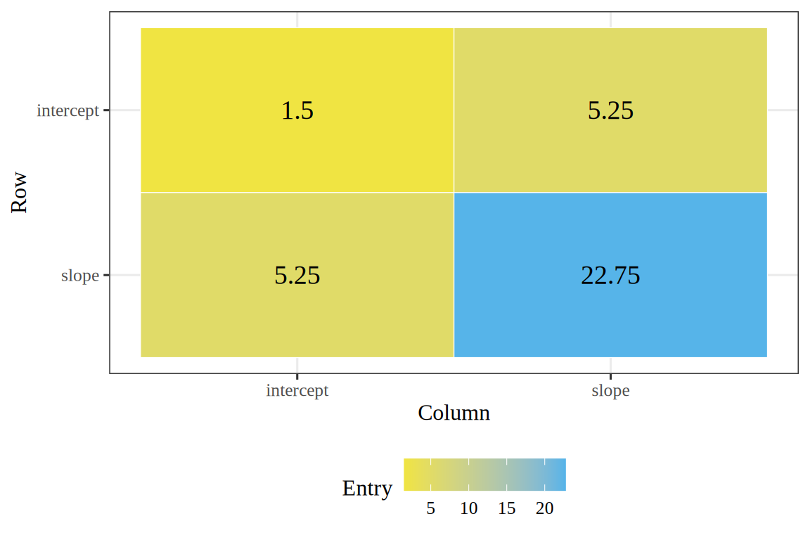
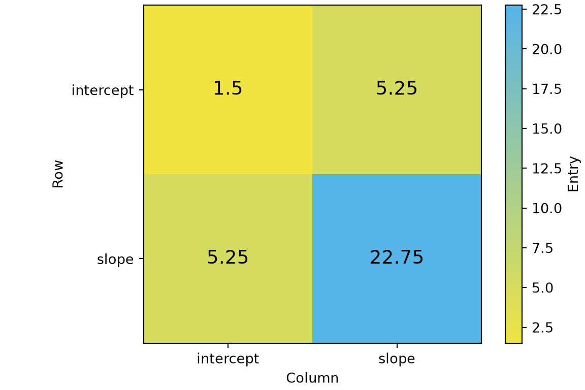
Figure 15: The Hessian of Example 22 at zero coefficients. The slope entry is far larger than the intercept entry because it sums the squared values of the feature.
(a)
Heat map of the two by two Hessian matrix at zero coefficients, with the entries printed in the cells. The intercept entry in the top left is 1.5, the two off-diagonal entries are both 5.25, and the slope entry in the bottom right is 22.75. The cells shade from yellow for 1.5 to blue for 22.75.
(b)
Heat map of the two by two Hessian matrix at zero coefficients, with the entries printed in the cells. The intercept entry in the top left is 1.5, the two off-diagonal entries are both 5.25, and the slope entry in the bottom right is 22.75. The cells shade from yellow for 1.5 to blue for 22.75.

The Hessian changes with the coefficients. Figure 16 shows its smallest eigenvalue, after subtracting 3.5 from every predictor value, over the intercept and the slope.

Show code
x_six <- 1:6 - 3.5
y_six <- c(0, 0, 1, 0, 1, 1)
# nolint next: undesirable_function_linter.
design_six <- cbind(1, x_six)
intercepts_six <- seq(-3, 3, length.out = 150)
slopes_six <- seq(-0.5, 3, length.out = 150)
grid_six <- tidyr::expand_grid(intercept = intercepts_six, slope = slopes_six)
# nolint next: undesirable_function_linter.
coef_mat <- rbind(grid_six$intercept, grid_six$slope)
prob_mat <- stats::plogis(design_six %*% coef_mat)
weight_mat <- prob_mat * (1 - prob_mat)
entry_top_left <- colSums(weight_mat)
entry_off_diag <- colSums(weight_mat * x_six)
entry_bottom_right <- colSums(weight_mat * x_six^2)
determinant <- entry_top_left * entry_bottom_right - entry_off_diag^2
half_gap <- (entry_top_left - entry_bottom_right) / 2
eigen_mean <- (entry_top_left + entry_bottom_right) / 2
eigen_max <- eigen_mean + sqrt(half_gap^2 + entry_off_diag^2)
hessian_six <- dplyr::mutate(
  grid_six,
  log_eigen_min = log10(determinant / eigen_max)
)
fit_six <- stats::glm(y_six ~ x_six, family = stats::binomial)
fit_coef <- stats::coef(fit_six)
mle_six <- tibble::tibble(
  intercept = fit_coef[1],
  slope = fit_coef[2]
)
hessian_six |>
  ggplot2::ggplot() +
  ggplot2::aes(intercept, slope, fill = log_eigen_min) +
  ggplot2::geom_raster() +
  ggplot2::geom_point(
    data = mle_six,
    mapping = ggplot2::aes(intercept, slope),
    inherit.aes = FALSE,
    shape = 18,
    size = 4
  ) +
  ggplot2::scale_fill_viridis_c() +
  ggplot2::labs(
    x = "Intercept",
    y = "Slope",
    fill = "log10 of the\nsmallest\neigenvalue"
  )
Show code
import matplotlib.pyplot as plt
import numpy as np
import statsmodels.api as sm

x_six = np.arange(1, 7) - 3.5
y_six = np.array([0, 0, 1, 0, 1, 1])
design_six = sm.add_constant(x_six.astype(float))
intercepts = np.linspace(-3, 3, 300)
slopes = np.linspace(-0.5, 3, 300)
grid_intercept, grid_slope = np.meshgrid(intercepts, slopes)
coef_grid = np.stack([grid_intercept.ravel(), grid_slope.ravel()])
prob_grid = 1 / (1 + np.exp(-(design_six @ coef_grid)))
weight_grid = prob_grid * (1 - prob_grid)
entry_top_left = weight_grid.sum(axis=0)
entry_off_diag = (weight_grid * x_six[:, None]).sum(axis=0)
entry_bottom_right = (weight_grid * x_six[:, None] ** 2).sum(axis=0)
determinant = entry_top_left * entry_bottom_right - entry_off_diag**2
half_gap = (entry_top_left - entry_bottom_right) / 2
eigen_max = (entry_top_left + entry_bottom_right) / 2 + np.sqrt(half_gap**2 + entry_off_diag**2)
log_eigen_min = np.log10(determinant / eigen_max).reshape(grid_intercept.shape)
fit_six = sm.GLM(y_six, design_six, family=sm.families.Binomial()).fit()
fig, ax = plt.subplots(figsize=(6, 4), layout="constrained")
image = ax.pcolormesh(
    grid_intercept, grid_slope, log_eigen_min, cmap="viridis", shading="auto"
)
ax.plot(fit_six.params[0], fit_six.params[1], "kD", markersize=8);
ax.set_xlabel("Intercept");
ax.set_ylabel("Slope");
fig.colorbar(image, ax=ax, label="log10 of the smallest eigenvalue");
plt.show()
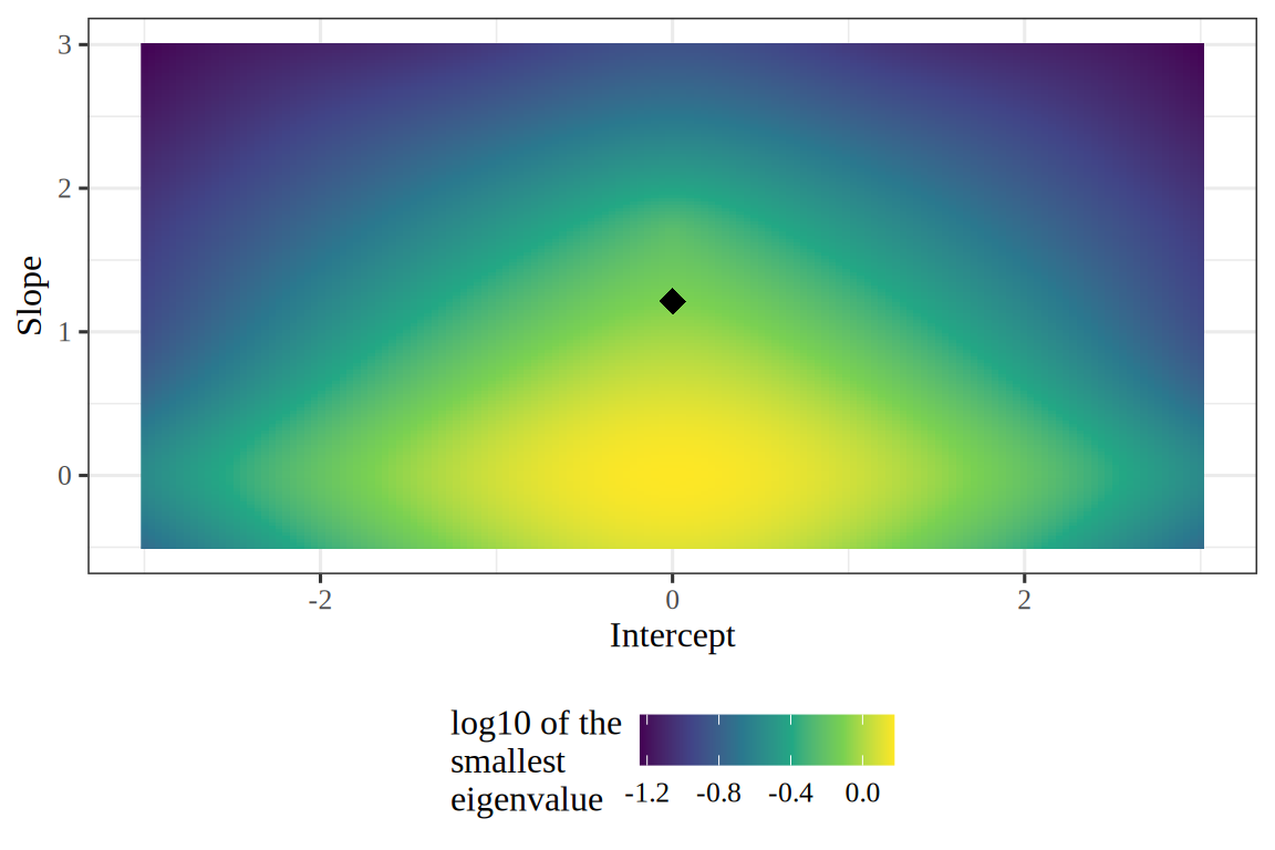
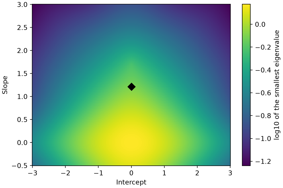
Figure 16: The smallest eigenvalue of the Hessian of the total log loss for the six points of Example 21, over the intercept and the slope. The maximum likelihood estimate is in black. The smallest eigenvalue is above 0 at every vector of coefficients shown. It is largest at the zero coefficients, where every fitted probability is 1/2, and shrinks as any of them approaches 0 or 1.
(a)
Heat map of the base 10 logarithm of the smallest eigenvalue of the Hessian, over the intercept from -3 to 3 and the slope from -0.5 to 3. The values range from about -1.24 to 0.18, so the smallest eigenvalue is positive everywhere in the plane. The shading is lightest, with a value near 0.18, an eigenvalue of 1.5, around the origin, where every fitted probability is one half, and darkens in every direction away from it, most in the upper corners. A black diamond marks the maximum likelihood estimate, at an intercept of 0 and a slope of about 1.21.
(b)
Heat map of the base 10 logarithm of the smallest eigenvalue of the Hessian, over the intercept from -3 to 3 and the slope from -0.5 to 3. The values range from about -1.24 to 0.18, so the smallest eigenvalue is positive everywhere in the plane. The shading is lightest, with a value near 0.18, an eigenvalue of 1.5, around the origin, where every fitted probability is one half, and darkens in every direction away from it, most in the upper corners. A black diamond marks the maximum likelihood estimate, at an intercept of 0 and a slope of about 1.21.

Figure 17 draws the same smallest eigenvalue as a surface, so its height shows the curvature.

Show code
x_six <- 1:6 - 3.5
y_six <- c(0, 0, 1, 0, 1, 1)
# nolint next: undesirable_function_linter.
design_six <- cbind(1, x_six)
intercepts_six <- seq(-3, 3, length.out = 61)
slopes_six <- seq(-0.5, 3, length.out = 61)
grid_six <- tidyr::expand_grid(slope = slopes_six, intercept = intercepts_six)
# nolint next: undesirable_function_linter.
coef_mat <- rbind(grid_six$intercept, grid_six$slope)
prob_mat <- stats::plogis(design_six %*% coef_mat)
weight_mat <- prob_mat * (1 - prob_mat)
entry_top_left <- colSums(weight_mat)
entry_off_diag <- colSums(weight_mat * x_six)
entry_bottom_right <- colSums(weight_mat * x_six^2)
determinant <- entry_top_left * entry_bottom_right - entry_off_diag^2
half_gap <- (entry_top_left - entry_bottom_right) / 2
eigen_mean <- (entry_top_left + entry_bottom_right) / 2
eigen_max <- eigen_mean + sqrt(half_gap^2 + entry_off_diag^2)
n_intercepts <- length(intercepts_six)
eigen_min <- matrix(determinant / eigen_max, ncol = n_intercepts, byrow = TRUE)
fit_six <- stats::glm(y_six ~ x_six, family = stats::binomial)
fit_coef <- stats::coef(fit_six)
fit_weight <- stats::fitted(fit_six) * (1 - stats::fitted(fit_six))
fit_hessian <- crossprod(design_six, fit_weight * design_six)
fit_eigen <- eigen(fit_hessian, symmetric = TRUE, only.values = TRUE)
mle_height <- min(fit_eigen$values)
mle_six <- tibble::tibble(
  intercept = fit_coef[1],
  slope = fit_coef[2],
  z = mle_height
)
mle_marker <- list(color = "#D55E00", size = 6, symbol = "diamond")
scale_stops <- c(0, 1)
grey_cols <- c("#E5E5E5", "#808080")
grey_scale <- list(scale_stops, grey_cols)
eye_six <- list(x = 1.7, y = -1.7, z = 0.9)
xaxis_six <- list(title = "Intercept")
yaxis_six <- list(title = "Slope")
zaxis_six <- list(title = "Smallest eigenvalue")
camera_six <- list(eye = eye_six)
scene_six <- list(
  xaxis = xaxis_six,
  yaxis = yaxis_six,
  zaxis = zaxis_six,
  camera = camera_six
)
legend_six <- list(orientation = "h")
plotly::plot_ly() |>
  plotly::add_surface(
    x = intercepts_six,
    y = slopes_six,
    z = eigen_min,
    colorscale = grey_scale,
    showscale = FALSE,
    opacity = 0.7
  ) |>
  plotly::add_markers(
    data = mle_six,
    x = ~intercept,
    y = ~slope,
    z = ~z,
    marker = mle_marker,
    name = "MLE"
  ) |>
  plotly::layout(scene = scene_six, legend = legend_six)
Show code
import html
import numpy as np
import plotly.graph_objects as go
import statsmodels.api as sm

fig_alt = r.hd3_alt_sf

x_six = np.arange(1, 7) - 3.5
y_six = np.array([0, 0, 1, 0, 1, 1])
design_six = sm.add_constant(x_six)
intercepts_six = np.linspace(-3, 3, 61)
slopes_six = np.linspace(-0.5, 3, 61)
grid_intercept, grid_slope = np.meshgrid(intercepts_six, slopes_six)
coef_grid = np.stack([grid_intercept.ravel(), grid_slope.ravel()])
prob_grid = 1 / (1 + np.exp(-(design_six @ coef_grid)))
weight_grid = prob_grid * (1 - prob_grid)
entry_top_left = weight_grid.sum(axis=0)
entry_off_diag = (weight_grid * x_six[:, None]).sum(axis=0)
entry_bottom_right = (weight_grid * x_six[:, None] ** 2).sum(axis=0)
determinant = entry_top_left * entry_bottom_right - entry_off_diag**2
half_gap = (entry_top_left - entry_bottom_right) / 2
eigen_mean = (entry_top_left + entry_bottom_right) / 2
eigen_max = eigen_mean + np.sqrt(half_gap**2 + entry_off_diag**2)
eigen_min = (determinant / eigen_max).reshape(grid_intercept.shape)
fit_six = sm.GLM(y_six, design_six, family=sm.families.Binomial()).fit()
fit_weight = fit_six.fittedvalues * (1 - fit_six.fittedvalues)
fit_hessian = design_six.T @ (fit_weight[:, None] * design_six)
mle_height = np.linalg.eigvalsh(fit_hessian).min()
fig = go.Figure(data=[
    go.Surface(x=intercepts_six, y=slopes_six, z=eigen_min,
               colorscale=[[0, "#E5E5E5"], [1, "#808080"]],
               showscale=False, opacity=0.7, showlegend=False),
    go.Scatter3d(x=[fit_six.params[0]], y=[fit_six.params[1]],
                 z=[mle_height], mode="markers", name="MLE",
                 marker=dict(color="#D55E00", size=4, symbol="diamond")),
])
fig.update_layout(
    scene=dict(
        xaxis_title="Intercept",
        yaxis_title="Slope",
        zaxis_title="Smallest eigenvalue",
        camera=dict(eye=dict(x=1.7, y=-1.7, z=0.9)),
    ),
    legend=dict(orientation="h"),
);
print(
    "```{=html}\n"
    + f'<div role="group" aria-label="{html.escape(fig_alt)}">\n'
    + fig.to_html(full_html=False, include_plotlyjs="cdn")
    + "\n</div>\n```"
)
Figure 17: The smallest eigenvalue of the Hessian of the total log loss for the six points of Example 21, as a surface over the intercept and the slope. The maximum likelihood estimate is in vermilion.
(a)

Example 23 (The total log loss, its gradient and its Hessian on the WCGS data)

Example 23 (The total log loss, its gradient and its Hessian on the WCGS data) Consider a logistic regression model of coronary heart disease (chd) in the WCGS data with two features, age and body mass index (BMI). The earlier examples on this page use age alone or BMI alone, and this one uses both. Center each feature at its sample mean, 46.28 years and 24.52 kg/m\(^2\), so that \(\prob_\iobs = \sigmoidf{\coef{0} + \coef{\text{age}} \predvar_{\iobs,\text{age}} + \coef{\text{BMI}} \predvar_{\iobs,\text{BMI}}}\), where \(\predvar_{\iobs,\text{age}}\) and \(\predvar_{\iobs,\text{BMI}}\) are man \(\iobs\)’s centered age and BMI. Centering makes \(\coef{0}\) the log-odds of a man whose age and BMI are both at their sample means. It also keeps the surfaces below readable. They hold the intercept fixed and vary the two slopes. With uncentered ages, a change of \(0.1\) in \(\coef{\text{age}}\) would move every man’s log-odds by about 4.6, and the total log loss \(C\) would rise steeply on either side of one narrow valley. The maximum likelihood fit is \(\hcoef{0} = -2.514\), \(\hcoef{\text{age}} = 0.0739\) and \(\hcoef{\text{BMI}} = 0.0815\).

Figure 18 starts at that fit. Its top three panels compare the fitted curve at the sample mean BMI with the proportion of men with the disease at each age. The curve rises with age on the probability scale (Figure 18 (a)) and curves upward on the odds scale (Figure 18 (b)), and on the log-odds scale (Figure 18 (c)) it is a straight line with slope \(\coef{\text{age}}\). Its bottom three panels draw \(C\) over the two slopes, the two slope entries of its gradient from Theorem 11, and the three distinct slope entries of its Hessian from Theorem 12.

  • The total log loss is a bowl (Figure 18 (d)). The sliders start at the maximum likelihood fit, so the black marker starts at the bottom of the bowl. There both gradient surfaces cross the gray plane at height \(0\) (Figure 18 (e)): both gradient entries round to 0 at four decimal places.
  • The bowl is steeper along \(\coef{\text{age}}\). The slope of each gradient surface along its own coefficient is the matching diagonal Hessian entry, 8672 for age and 1739 for BMI at the fit (Figure 18 (f)). Each entry is a weighted sum of a squared centered feature, and the sample standard deviation of age, in years, is 2.2 times that of BMI, in kg/m\(^2\).
  • The cross entry is small. At the fit \(\xderivf{C}{\coef{\text{age}}}{\coef{\text{BMI}}} = 241\), because the sample correlation of age and BMI in the WCGS men is only 0.027.

Each surface depends on all three coefficients, so moving the intercept slider changes every surface, while moving a slope slider moves only the black markers.

Figure 18: The logistic regression model of Example 23, for coronary heart disease with centered age and BMI as features. The top three panels show, at each age, the proportion of men with the disease, as dots, and the fitted curve at the sample mean BMI, in vermilion, on the probability, odds and log-odds scales. The bottom three panels show, over the two slopes at a fixed intercept, the total log loss \(C\), the two slope entries of its gradient (age in blue, BMI in vermilion), and the three distinct slope entries of its Hessian (age twice in blue, BMI twice in vermilion, one of each in green). The sliders between the top and bottom panels choose the three coefficients and start at the maximum likelihood fit; black markers show their values on each surface, and turning any surface turns the others with it.
(a) The probability scale
(b) The odds scale
(c) The log-odds scale
(d) The total log loss
(e) The gradient
(f) The Hessian

Theorem 13 (The Hessian of the total log loss has bounded eigenvalues)

Theorem 13 (The Hessian of the total log loss has bounded eigenvalues) For every \(\vcoef\), every eigenvalue of the Hessian of the total log loss is at most

\[ \tfrac{1}{4}\eigvalmaxf{\stprod{\design}}. \]

Proof

Proof. By Theorem 12, the Hessian is \(\tp{\design} W \design\), with \(W = \diagf{\prob_i(1-\prob_i)}\). Part 4d of the sigmoid properties exercise showed that every \(\prob_i(1-\prob_i) \le 1/4\).

Let \(\vv\) be a unit eigenvector of \(\tp{\design} W \design\) for the eigenvalue \(\eigval\). Then \(\eigval = \tp{\vv} \tp{\design} W \design \vv\). Write \(z_i\) for the \(i\)th entry of \(\design \vv\). Then

\[ \eigval = \sumin \prob_i(1-\prob_i) z_i^2 \le \tfrac{1}{4} \sumin z_i^2 = \tfrac{1}{4} \tp{\vv} \stprod{\design} \vv \le \tfrac{1}{4}\eigvalmaxf{\stprod{\design}}. \]

The last step holds because \(\tp{\vv} \stprod{\design} \vv\) is at most the largest eigenvalue of \(\stprod{\design}\).

Example 24 (The eigenvalue bound for the six points)

Example 24 (The eigenvalue bound for the six points) Take the six points of Example 21, and the coefficients \(\vcoef = (-3.5, 1)\), which put \(\prob_1\) and \(\prob_6\) away from \(1/2\). The code compares the largest eigenvalue of the Hessian with \(\tfrac14 \eigvalmaxf{\stprod{\design}}\).

# the six points, with the column of ones for the intercept
x_six <- 1:6
design_six <- cbind(1, x_six) # nolint
# the bound: a quarter of the largest eigenvalue of design' design
gram_six <- crossprod(design_six)
gram_eigen <- eigen(gram_six, symmetric = TRUE, only.values = TRUE)
gram_max <- max(gram_eigen$values)
# the Hessian at the coefficients (-3.5, 1)
coef_far <- c(-3.5, 1)
linear_mat <- design_six %*% coef_far
linear_far <- drop(linear_mat)
p_far <- plogis(linear_far)
w_far <- p_far * (1 - p_far)
hessian_far <- crossprod(design_six, w_far * design_six)
hessian_eigen <- eigen(hessian_far, symmetric = TRUE, only.values = TRUE)
hessian_max <- max(hessian_eigen$values)
c(hessian_max = hessian_max, bound = gram_max / 4)
hessian_max       bound 
   13.59139    23.97629 
import numpy as np

# the six points, with the column of ones for the intercept
x_six = np.arange(1, 7)
design_six = np.column_stack([np.ones(6), x_six])
# the bound: a quarter of the largest eigenvalue of design' design
gram_six = design_six.T @ design_six
gram_max = np.linalg.eigvalsh(gram_six).max()
# the Hessian at the coefficients (-3.5, 1)
coef_far = np.array([-3.5, 1.0])
linear_far = design_six @ coef_far
p_far = 1 / (1 + np.exp(-linear_far))
w_far = p_far * (1 - p_far)
hessian_far = design_six.T @ (w_far[:, None] * design_six)
hessian_max = np.linalg.eigvalsh(hessian_far).max()
print(hessian_max, gram_max / 4)
13.591392199129405 23.976292123646264

The largest eigenvalue of the Hessian is 13.591, which is below 23.976. At \(\vcoef = \vzero\) every \(\prob_i = 1/2\), so the Hessian is \(\tfrac14 \stprod{\design}\) and the two are equal.

Corollary 1 (A step size that is safe for every coefficient vector)

Corollary 1 (A step size that is safe for every coefficient vector) Gradient descent on the total log loss with the step size

\[\learnrate < \frac{8}{\eigvalmaxf{\stprod{\design}}}\]

lowers the loss at every step that starts from a \(\vcoef\) with a nonzero gradient.

Proof

Proof. Write \(C\) for the total log loss and \(L = \tfrac{1}{4}\eigvalmaxf{\stprod{\design}}\), so that \(\learnrate < 2/L\) is the condition \(\learnrate < 8/\eigvalmaxf{\stprod{\design}}\). Let \(\vg = \grad C(\vcoef)\) be nonzero, and take the step \(\vd = -\learnrate \vg\).

The Taylor expansion of \(C\) to second order, with a remainder, says that for some \(\vcoef'\) on the segment from \(\vcoef\) to \(\vcoef + \vd\),

\[C(\vcoef + \vd) = C(\vcoef) + \tp{\vg}\vd + \tfrac{1}{2}\tp{\vd}\paren{\grad^2 C(\vcoef')}\vd.\]

By Theorem 12 the Hessian is positive semidefinite, and by Theorem 13 its eigenvalues are at most \(L\), so \(\tfrac{1}{2}\tp{\vd}\paren{\grad^2 C(\vcoef')}\vd \le \tfrac{L}{2}\tp{\vd}\vd\). Substituting \(\vd = -\learnrate \vg\) gives

\[C(\vcoef + \vd) \le C(\vcoef) - \learnrate\paren{1 - \tfrac{L\learnrate}{2}}\tp{\vg}\vg.\]

Because \(\learnrate < 2/L\), the factor \(1 - L\learnrate/2\) is greater than zero, and \(\tp{\vg}\vg > 0\), so \(C\) falls.

Example 25 (The safe step size for the six points)

Example 25 (The safe step size for the six points) For the six points of Example 21, the step-size condition of Corollary 1 is \(\learnrate < 8/\eigvalmaxf{\stprod{\design}}\).

# the six points, with the column of ones for the intercept
x_six <- 1:6
design_six <- cbind(1, x_six) # nolint
# the largest eigenvalue of design' design
gram_six <- crossprod(design_six)
gram_eigen <- eigen(gram_six, symmetric = TRUE, only.values = TRUE)
gram_max <- max(gram_eigen$values)
# the safe step-size limit
8 / gram_max
[1] 0.08341573
import numpy as np

# the six points, with the column of ones for the intercept
x_six = np.arange(1, 7)
design_six = np.column_stack([np.ones(6), x_six])
# the largest eigenvalue of design' design
gram_max = np.linalg.eigvalsh(design_six.T @ design_six).max()
# the safe step-size limit
print(8 / gram_max)
0.08341573374590017

The largest eigenvalue of \(\stprod{\design}\) is 95.91, so every \(\learnrate\) below 0.0834 is safe at every \(\vcoef\).

Remark 5 (The safe step size is often too small)

Remark 5 (The safe step size is often too small). The condition of Corollary 1 holds for every \(\vcoef\), so it is often smaller than needed. In practice, a line search chooses step sizes adaptively without computing \(\eigvalmaxf{\stprod{\design}}\).

Theorem 14 (The residuals are orthogonal to every column of the design matrix at a minimizer)

Theorem 14 (The residuals are orthogonal to every column of the design matrix at a minimizer) At any finite minimizer \(\hat{\vcoef}\) of the total log loss, the gradient equals the zero vector:

\[ \tp{\design} \paren{\vprob - \voutvar} = \vzero. \]

Each column of \(\design\) is orthogonal to the vector of residuals, and the column of ones makes the residuals sum to zero.

Proof

Proof. The log loss is differentiable and \(\hat{\vcoef}\) minimizes it over all coefficient vectors, so its gradient vanishes there. By Theorem 11, \(\grad C(\hat{\vcoef}) = \tp{\design} \paren{\vprob - \voutvar}\). The \(j\)th entry of this vector is the dot product of the \(j\)th column of \(\design\) with the residuals, and the entry for the column of ones is \(\sumin \paren{\prob_i - \outvar_i}\).

Example 26 (Residuals at the fitted coefficients)

Example 26 (Residuals at the fitted coefficients) Fit a logistic regression with an intercept to the six points of Example 21, and compute \(\tp{\design} \paren{\vprob - \voutvar}\).

# the six points
x_six <- 1:6
y_six <- c(0, 0, 1, 0, 1, 1)
# the fit, and its design matrix with the column of ones
fit_six <- glm(y_six ~ x_six, family = binomial)
design_six <- model.matrix(fit_six)
# the residuals: fitted probabilities minus labels
residual_six <- fitted(fit_six) - y_six
# the gradient, rounded to six decimals
round(drop(crossprod(design_six, residual_six)), 6)
(Intercept)       x_six 
          0           0 
import numpy as np
import statsmodels.api as sm

# the six points
x_six = np.arange(1, 7)
y_six = np.array([0, 0, 1, 0, 1, 1])
# the fit, and its design matrix with the column of ones
design_six = sm.add_constant(x_six.astype(float))
fit_six = sm.GLM(y_six, design_six, family=sm.families.Binomial()).fit()
# the residuals: fitted probabilities minus labels
residual_six = fit_six.fittedvalues - y_six
# the gradient, rounded to six decimals
# adding 0.0 turns a negative zero into 0, so the output prints 0. rather than -0.
print((design_six.T @ residual_six).round(6) + 0.0)
[0. 0.]

Both entries are zero to six decimals, as Theorem 14 requires.

Figure 19 draws one vertical segment for each of the six points.

Show code
library(ggplot2)
lst_pts <- data.frame(
  x = x_six,
  label = factor(y_six, levels = c(1, 0)),
  y = y_six,
  fitted = fitted(fit_six)
)
lst_curve <- data.frame(x = seq(1, 6, length.out = 100))
lst_curve$prob <- predict(
  fit_six,
  newdata = data.frame(x_six = lst_curve$x),
  type = "response"
)
ggplot(lst_pts, aes(x, y, colour = label)) +
  geom_line(data = lst_curve, aes(y = prob), colour = "grey50") +
  geom_segment(aes(xend = x, yend = fitted, linetype = label), linewidth = 1) +
  geom_point(aes(shape = label), size = 3) +
  scale_colour_manual(values = c("1" = "#0072B2", "0" = "#D55E00")) +
  scale_shape_manual(values = c("1" = 16, "0" = 17)) +
  scale_linetype_manual(values = c("1" = "solid", "0" = "dashed")) +
  scale_x_continuous(breaks = 1:6) +
  labs(x = "Predictor", y = "Label and fitted probability", colour = "Label", shape = "Label",
       linetype = "Label")
Show code
import matplotlib.pyplot as plt

points_lst = r.lst_pts
curve_lst = r.lst_curve
fig, ax = plt.subplots(figsize=(6, 4), layout="constrained")
ax.plot(curve_lst["x"], curve_lst["prob"], color="grey");
for label_lst, colour, marker, style in [(1, "#0072B2", "o", "-"), (0, "#D55E00", "^", "--")]:
    keep_lst = points_lst["y"] == label_lst
    sub_lst = points_lst[keep_lst]
    ax.vlines(sub_lst["x"], sub_lst["fitted"], sub_lst["y"], color=colour, linestyle=style,
              linewidth=2);
    ax.plot(sub_lst["x"], sub_lst["y"], color=colour, marker=marker, markersize=8,
            linestyle="", label=f"label {label_lst}");
ax.set_xticks(range(1, 7));
ax.set_xlabel("Predictor");
ax.set_ylabel("Label and fitted probability");
fig.legend(loc="outside lower center", ncol=2);
plt.show()
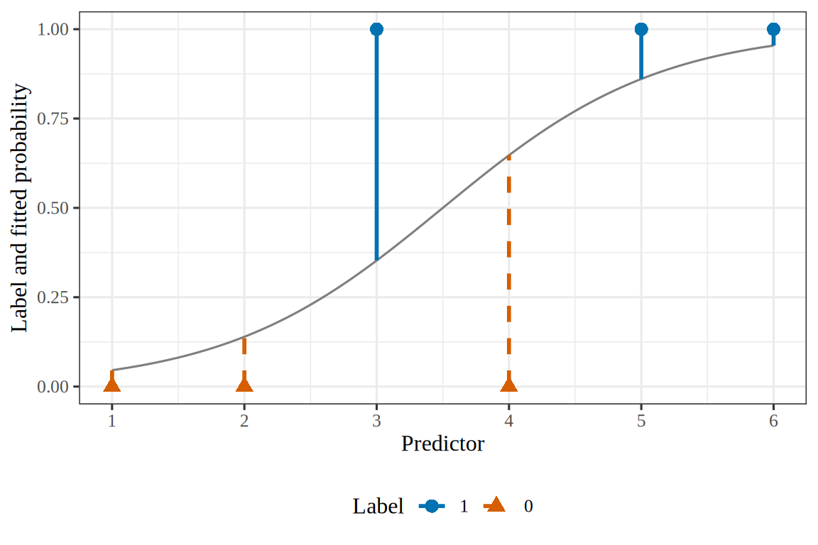
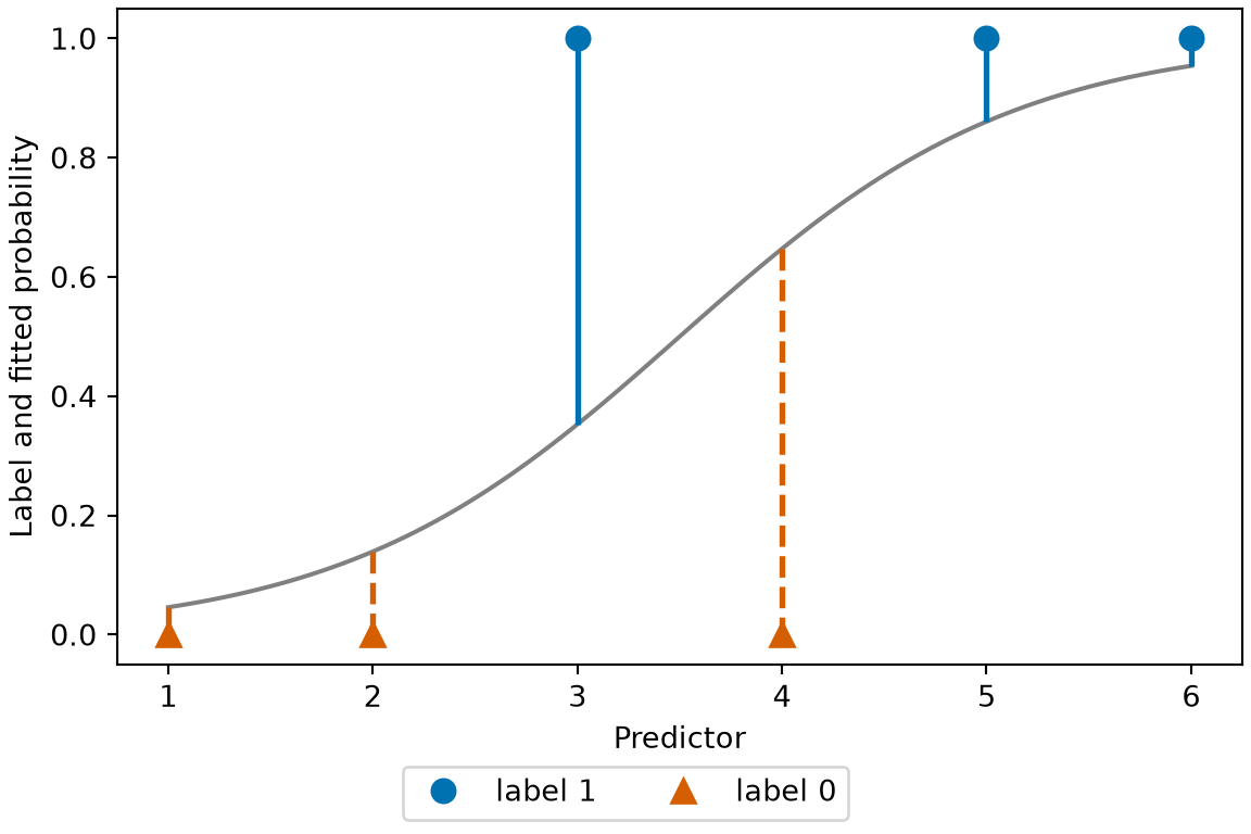
Figure 19: The six points of Example 26 and their fitted probability (curve). Each vertical segment is the residual of one point. The solid segments and the dashed segments have the same total length, because the intercept entry of the gradient is zero.
(a)
Plot of the label of six points against their predictor value, 1 to 6, with a grey S-shaped curve, the fitted probability, rising from about 0.05 at 1 to about 0.95 at 6. Blue circles at the label 1 mark the points at 3, 5 and 6, and vermilion triangles at the label 0 mark the points at 1, 2 and 4. A vertical segment joins each point to the curve. The segments of the points at the label 1 are solid and those of the points at the label 0 are dashed. The two longest segments, both about 0.65, belong to the points at 3 and 4, which the curve misses by the most.
(b)
Plot of the label of six points against their predictor value, 1 to 6, with a grey S-shaped curve, the fitted probability, rising from about 0.05 at 1 to about 0.95 at 6. Blue circles at the label 1 mark the points at 3, 5 and 6, and vermilion triangles at the label 0 mark the points at 1, 2 and 4. A vertical segment joins each point to the curve. The segments of the points at the label 1 are solid and those of the points at the label 0 are dashed. The two longest segments, both about 0.65, belong to the points at 3 and 4, which the curve misses by the most.

The score is this gradient with its sign reversed. Figure 20 draws the coefficients where each entry of the score is zero. It first subtracts 3.5 from every predictor value. This leaves the slope unchanged and moves the intercept to 0, the fitted log-odds at the predictor value 3.5. Without it, the two curves nearly coincide and are hard to tell apart. The two curves cross only at the fitted coefficients.

Show code
x_six <- 1:6 - 3.5
y_six <- c(0, 0, 1, 0, 1, 1)
# nolint next: undesirable_function_linter.
design_six <- cbind(1, x_six)
intercepts_six <- seq(-3, 3, length.out = 150)
slopes_six <- seq(-0.5, 3, length.out = 150)
grid_six <- tidyr::expand_grid(intercept = intercepts_six, slope = slopes_six)
# nolint next: undesirable_function_linter.
coef_mat <- rbind(grid_six$intercept, grid_six$slope)
prob_mat <- stats::plogis(design_six %*% coef_mat)
score_mat <- crossprod(design_six, y_six - prob_mat)
score_six <- dplyr::mutate(
  grid_six,
  score_intercept = score_mat[1, ],
  score_slope = score_mat[2, ]
)
fit_six <- stats::glm(y_six ~ x_six, family = stats::binomial)
fit_coef <- stats::coef(fit_six)
mle_six <- tibble::tibble(
  intercept = fit_coef[1],
  slope = fit_coef[2]
)
colours_six <- c("intercept" = "#0072B2", "slope" = "#D55E00")
linetypes_six <- c("intercept" = "solid", "slope" = "dashed")
score_six |>
  ggplot2::ggplot() +
  ggplot2::aes(intercept, slope) +
  ggplot2::geom_contour(
    ggplot2::aes(
      z = score_intercept,
      colour = "intercept",
      linetype = "intercept"
    ),
    breaks = 0 # check-unexplained-choices: allow
  ) +
  ggplot2::geom_contour(
    ggplot2::aes(z = score_slope, colour = "slope", linetype = "slope"),
    breaks = 0 # check-unexplained-choices: allow
  ) +
  ggplot2::geom_point(
    data = mle_six,
    shape = 18,
    size = 4
  ) +
  ggplot2::scale_colour_manual(values = colours_six) +
  ggplot2::scale_linetype_manual(values = linetypes_six) +
  ggplot2::labs(
    x = "Intercept",
    y = "Slope",
    colour = "Score component\nequal to zero",
    linetype = "Score component\nequal to zero"
  )
Show code
import matplotlib.pyplot as plt
import numpy as np
import statsmodels.api as sm
from matplotlib.lines import Line2D

x_six = np.arange(1, 7) - 3.5
y_six = np.array([0, 0, 1, 0, 1, 1])
design_six = sm.add_constant(x_six.astype(float))
intercepts = np.linspace(-3, 3, 300)
slopes = np.linspace(-0.5, 3, 300)
grid_intercept, grid_slope = np.meshgrid(intercepts, slopes)
coef_grid = np.stack([grid_intercept.ravel(), grid_slope.ravel()])
prob_grid = 1 / (1 + np.exp(-(design_six @ coef_grid)))
score_grid = design_six.T @ (y_six[:, None] - prob_grid)
fit_six = sm.GLM(y_six, design_six, family=sm.families.Binomial()).fit()
fig, ax = plt.subplots(figsize=(6, 4), layout="constrained")
for row, colour, style in [(0, "#0072B2", "-"), (1, "#D55E00", "--")]:
    ax.contour(
        grid_intercept,
        grid_slope,
        score_grid[row].reshape(grid_intercept.shape),
        levels=[0],
        colors=colour,
        linestyles=style,
    );
ax.plot(fit_six.params[0], fit_six.params[1], "kD", markersize=8);
ax.set_xlabel("Intercept");
ax.set_ylabel("Slope");
handles = [
    Line2D([], [], color="#0072B2", linestyle="-", label="intercept"),
    Line2D([], [], color="#D55E00", linestyle="--", label="slope"),
]
fig.legend(
    handles=handles,
    title="Score component equal to zero",
    loc="outside lower center",
    ncol=2,
);
plt.show()
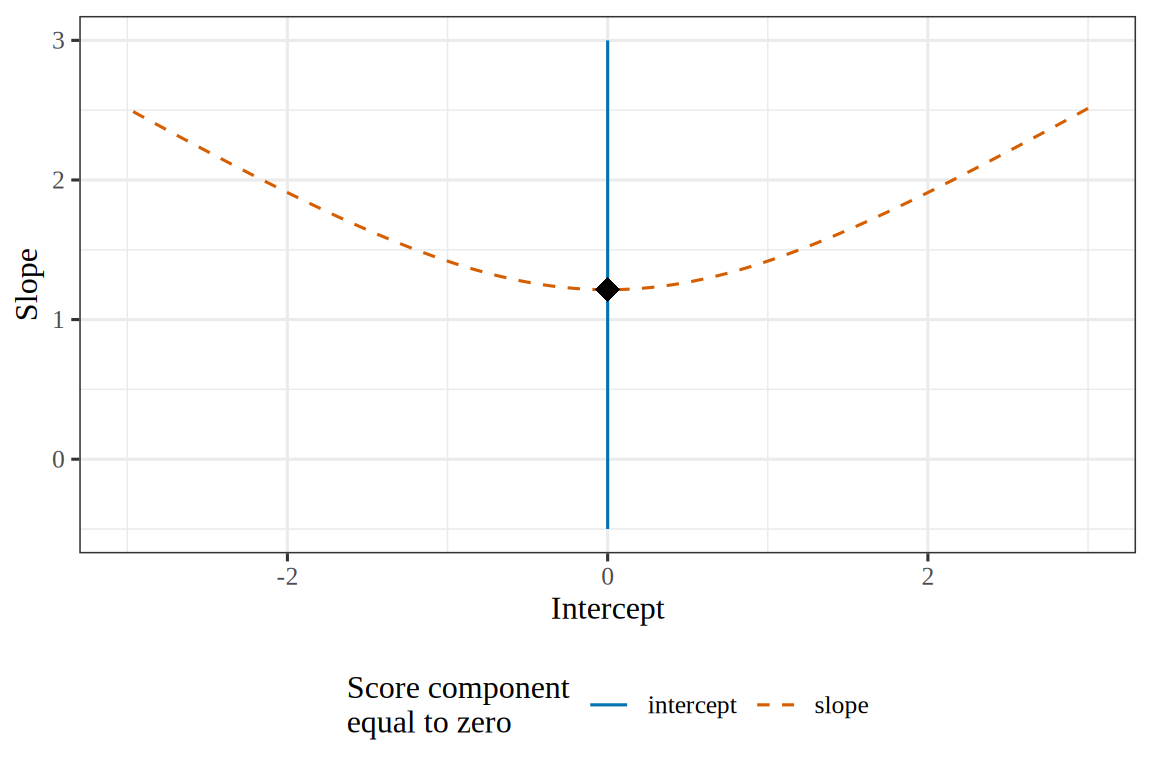
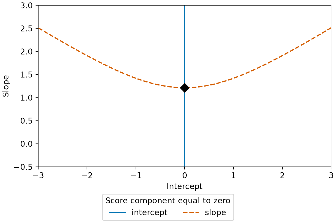
Figure 20: The score of the log-likelihood for the six points of Example 21, over the intercept and the slope. Each curve marks the coefficients where one entry of the score is zero. The maximum likelihood estimate, in black, is the one point where both entries are zero.
(a)
Plot of the slope against the intercept, with two curves. The solid blue curve marks the coefficients where the intercept component of the score is zero, and the dashed vermilion curve marks the coefficients where the slope component is zero. The curves cross at one black diamond, the maximum likelihood estimate, at an intercept of 0 and a slope of about 1.21.
(b)
Plot of the slope against the intercept, with two curves. The solid blue curve marks the coefficients where the intercept component of the score is zero, and the dashed vermilion curve marks the coefficients where the slope component is zero. The curves cross at one black diamond, the maximum likelihood estimate, at an intercept of 0 and a slope of about 1.21.

Figure 21 draws both entries of the score as surfaces, so the curves of Figure 20 are where the surfaces cross height 0.

Show code
x_six <- 1:6 - 3.5
y_six <- c(0, 0, 1, 0, 1, 1)
# nolint next: undesirable_function_linter.
design_six <- cbind(1, x_six)
intercepts_six <- seq(-3, 3, length.out = 61)
slopes_six <- seq(-0.5, 3, length.out = 61)
grid_six <- tidyr::expand_grid(slope = slopes_six, intercept = intercepts_six)
# nolint next: undesirable_function_linter.
coef_mat <- rbind(grid_six$intercept, grid_six$slope)
prob_mat <- stats::plogis(design_six %*% coef_mat)
score_mat <- crossprod(design_six, y_six - prob_mat)
n_intercepts <- length(intercepts_six)
score_intercept <- matrix(score_mat[1, ], ncol = n_intercepts, byrow = TRUE)
score_slope <- matrix(score_mat[2, ], ncol = n_intercepts, byrow = TRUE)
fit_six <- stats::glm(y_six ~ x_six, family = stats::binomial)
fit_coef <- stats::coef(fit_six)
mle_six <- tibble::tibble(
  intercept = fit_coef[1],
  slope = fit_coef[2],
  z = 0
)
mle_marker <- list(color = "black", size = 6, symbol = "diamond")
scale_stops <- c(0, 1)
blue_cols <- c("#0072B2", "#0072B2")
blue_scale <- list(scale_stops, blue_cols)
vermilion_cols <- c("#D55E00", "#D55E00")
vermilion_scale <- list(scale_stops, vermilion_cols)
eye_six <- list(x = 1.7, y = -1.7, z = 0.9)
xaxis_six <- list(title = "Intercept")
yaxis_six <- list(title = "Slope")
zaxis_six <- list(title = "Score component")
camera_six <- list(eye = eye_six)
scene_six <- list(
  xaxis = xaxis_six,
  yaxis = yaxis_six,
  zaxis = zaxis_six,
  camera = camera_six
)
legend_six <- list(orientation = "h")
plotly::plot_ly() |>
  plotly::add_surface(
    x = intercepts_six,
    y = slopes_six,
    z = score_intercept,
    colorscale = blue_scale,
    showscale = FALSE,
    opacity = 0.6,
    showlegend = TRUE,
    name = "intercept component"
  ) |>
  plotly::add_surface(
    x = intercepts_six,
    y = slopes_six,
    z = score_slope,
    colorscale = vermilion_scale,
    showscale = FALSE,
    opacity = 0.6,
    showlegend = TRUE,
    name = "slope component"
  ) |>
  plotly::add_markers(
    data = mle_six,
    x = ~intercept,
    y = ~slope,
    z = ~z,
    marker = mle_marker,
    name = "MLE"
  ) |>
  plotly::layout(scene = scene_six, legend = legend_six)
Show code
import html
import numpy as np
import plotly.graph_objects as go
import statsmodels.api as sm

fig_alt = r.sc3_alt_sf

x_six = np.arange(1, 7) - 3.5
y_six = np.array([0, 0, 1, 0, 1, 1])
design_six = sm.add_constant(x_six)
intercepts_six = np.linspace(-3, 3, 61)
slopes_six = np.linspace(-0.5, 3, 61)
grid_intercept, grid_slope = np.meshgrid(intercepts_six, slopes_six)
coef_grid = np.stack([grid_intercept.ravel(), grid_slope.ravel()])
prob_grid = 1 / (1 + np.exp(-(design_six @ coef_grid)))
score_grid = design_six.T @ (y_six[:, None] - prob_grid)
fit_six = sm.GLM(y_six, design_six, family=sm.families.Binomial()).fit()
fig = go.Figure(data=[
    go.Surface(x=intercepts_six, y=slopes_six,
               z=score_grid[0].reshape(grid_intercept.shape),
               colorscale=[[0, "#0072B2"], [1, "#0072B2"]],
               showscale=False, opacity=0.6, name="intercept component",
               showlegend=True),
    go.Surface(x=intercepts_six, y=slopes_six,
               z=score_grid[1].reshape(grid_intercept.shape),
               colorscale=[[0, "#D55E00"], [1, "#D55E00"]],
               showscale=False, opacity=0.6, name="slope component",
               showlegend=True),
    go.Scatter3d(x=[fit_six.params[0]], y=[fit_six.params[1]], z=[0],
                 mode="markers", name="MLE",
                 marker=dict(color="black", size=4, symbol="diamond")),
])
fig.update_layout(
    scene=dict(
        xaxis_title="Intercept",
        yaxis_title="Slope",
        zaxis_title="Score component",
        camera=dict(eye=dict(x=1.7, y=-1.7, z=0.9)),
    ),
    legend=dict(orientation="h"),
);
print(
    "```{=html}\n"
    + f'<div role="group" aria-label="{html.escape(fig_alt)}">\n'
    + fig.to_html(full_html=False, include_plotlyjs="cdn")
    + "\n</div>\n```"
)
Figure 21: The score of the log-likelihood for the six points of Example 21, as surfaces over the intercept and the slope. The maximum likelihood estimate, in black, is the one point where both surfaces are at height 0.
(a)

Exercise 43 (Fitting by gradient descent, in code)

Exercise 43 (Fitting by gradient descent, in code) Simulate \(n = 400\) observations with two standard normal features \(x_1, x_2\) and labels drawn from \(\Pr[Y = 1 \mid \vx] = \sigmoid(-0.5 + 2x_1 - 1.5x_2)\), so the coefficients that generated the data are \(\vcoef = (-0.5, 2, -1.5)\).

In Python, R or Julia, minimize the mean log loss \(J(\vcoef) = \tfrac1\nobs\sum_i C_i\) by gradient descent from \(\vcoef = \vzero\), with step size \(\learnrate = 0.5\) for \(10{,}000\) steps, using the gradient of Exercise 34. Explain how the sign and scale of the gradient of \(J\) relate to the gradient \(\tp{\design(\mx)}(\vy - \vprob)\) of the log-likelihood of Exercise 3.

Solution 43. The gradient of \(J\) is \(\tp{\design(\mx)}(\vprob - \vy)/n\). It is the log-likelihood’s gradient \(\tp{\design(\mx)}(\vy - \vprob)\) with its sign reversed, because \(J\) is the negative log-likelihood, and divided by \(n\), because \(J\) is a mean. Dividing by \(\nobs\) does not change the minimizer (Exercise 21), and it makes a good step size depend less on how many observations there are.

import numpy as np

sigmoid = lambda z: 0.5 * (1 + np.tanh(0.5 * z))

rng = np.random.default_rng(0)
n = 400
x1, x2 = rng.normal(size=n), rng.normal(size=n)
X = np.column_stack([np.ones(n), x1, x2])
y = (rng.random(n) < sigmoid(-0.5 + 2 * x1 - 1.5 * x2)).astype(float)

def J(b):
    p = sigmoid(X @ b)
    return -np.mean(y * np.log(p) + (1 - y) * np.log(1 - p))

def grad_J(b):
    return X.T @ (sigmoid(X @ b) - y) / n

beta = np.zeros(3)
for _ in range(10_000):
    beta = beta - 0.5 * grad_J(beta)

print(beta.round(2))          # true values: [-0.5, 2, -1.5]
[-0.54  1.95 -1.18]
print(J(beta).round(4))
0.4294
sigmoid <- function(z) 0.5 * (1 + tanh(0.5 * z))

set.seed(0)
n <- 400
x1 <- rnorm(n)
x2 <- rnorm(n)
X <- cbind(1, x1, x2) # nolint: object_name_linter. X matches the prose.
y <- as.numeric(runif(n) < sigmoid(-0.5 + 2 * x1 - 1.5 * x2))

J <- function(b) { # nolint: object_name_linter.
  p <- sigmoid(drop(X %*% b))
  -mean(y * log(p) + (1 - y) * log(1 - p))
}

grad_J <- function(b) drop(t(X) %*% (sigmoid(drop(X %*% b)) - y) / n) # nolint

beta <- c(0, 0, 0)
for (step in seq_len(10000)) beta <- beta - 0.5 * grad_J(beta)

round(beta, 2)                # true values: c(-0.5, 2, -1.5)
         x1    x2 
-0.53  1.98 -1.46 
round(J(beta), 4)
[1] 0.4201
using Random, LinearAlgebra, Statistics

sigmoid(z) = 0.5 .* (1 .+ tanh.(0.5 .* z));

Random.seed!(0);
n = 400;
x1, x2 = randn(n), randn(n);
X = [ones(n) x1 x2];
y = Float64.(rand(n) .< sigmoid(-0.5 .+ 2 .* x1 .- 1.5 .* x2));

function J(b)
    p = sigmoid(X * b)
    -mean(y .* log.(p) .+ (1 .- y) .* log.(1 .- p))
end;

grad_J(b) = X' * (sigmoid(X * b) .- y) ./ n;

beta = zeros(3);
for _ in 1:10_000
    global beta = beta - 0.5 .* grad_J(beta)
end

println(round.(beta, digits = 2))   # true values: [-0.5, 2, -1.5]
[-0.48, 1.97, -1.62]
println(round(J(beta), digits = 4))
0.4069

Figure 22 plots \(J\) at each step, for the simulated data of this solution.

Show code
set.seed(0)
gdl_n <- 400
gdl_x1 <- rnorm(gdl_n)
gdl_x2 <- rnorm(gdl_n)
gdl_ones <- rep(1, gdl_n)
gdl_cols <- c(gdl_ones, gdl_x1, gdl_x2)
gdl_x <- matrix(gdl_cols, ncol = 3)
gdl_score <- -0.5 + 2 * gdl_x1 - 1.5 * gdl_x2
gdl_u <- runif(gdl_n)
gdl_y <- as.numeric(gdl_u < plogis(gdl_score))
gdl_beta <- c(0, 0, 0)
gdl_loss <- numeric(10000)
for (gdl_s in seq_along(gdl_loss)) {
  gdl_eta <- drop(gdl_x %*% gdl_beta)
  gdl_p <- plogis(gdl_eta)
  gdl_terms <- gdl_y * log(gdl_p) + (1 - gdl_y) * log(1 - gdl_p)
  gdl_loss[gdl_s] <- -mean(gdl_terms)
  gdl_resid <- gdl_p - gdl_y
  gdl_cross <- crossprod(gdl_x, gdl_resid)
  gdl_grad <- drop(gdl_cross) / gdl_n
  gdl_beta <- gdl_beta - 0.5 * gdl_grad
}
gdl_step <- seq_along(gdl_loss)
gdl_curve <- tibble::tibble(step = gdl_step, loss = gdl_loss)
gdl_start <- log(2)
gdl_curve |>
  ggplot2::ggplot(ggplot2::aes(step, loss)) +
  ggplot2::geom_hline(
    yintercept = gdl_start,
    linetype = "dashed",
    colour = "grey50"
  ) +
  ggplot2::geom_line(colour = "#0072B2") +
  ggplot2::scale_x_log10() +
  ggplot2::labs(x = "Step", y = "Mean log loss")
Show code
import matplotlib.pyplot as plt
import numpy as np
from scipy.special import expit

rng_gdl = np.random.default_rng(0)
n_gdl = 400
x1_gdl = rng_gdl.normal(size=n_gdl)
x2_gdl = rng_gdl.normal(size=n_gdl)
x_gdl = np.column_stack([np.ones(n_gdl), x1_gdl, x2_gdl])
score_gdl = -0.5 + 2 * x1_gdl - 1.5 * x2_gdl
y_gdl = (rng_gdl.random(n_gdl) < expit(score_gdl)).astype(float)
beta_gdl = np.zeros(3)
loss_gdl = np.zeros(10000)
for s in range(10000):
    p_gdl = expit(x_gdl @ beta_gdl)
    terms_gdl = y_gdl * np.log(p_gdl) + (1 - y_gdl) * np.log(1 - p_gdl)
    loss_gdl[s] = -np.mean(terms_gdl)
    beta_gdl = beta_gdl - 0.5 * x_gdl.T @ (p_gdl - y_gdl) / n_gdl

fig, ax = plt.subplots(figsize=(5, 3.5), layout="constrained")
ax.axhline(np.log(2), color="grey", linestyle="--");
ax.plot(np.arange(1, 10001), loss_gdl, color="#0072B2");
ax.set_xscale("log");
ax.set_xlabel("Step");
ax.set_ylabel("Mean log loss");
plt.show()
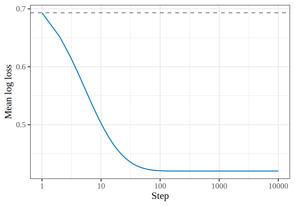
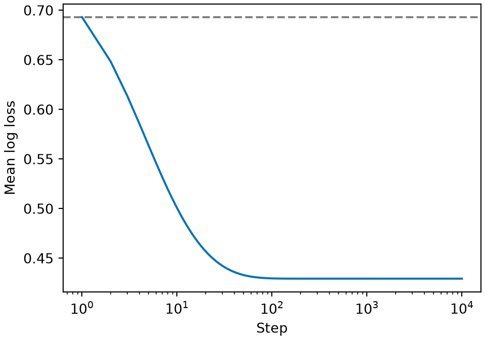
Figure 22: The mean log loss falls quickly at first and then stays at its minimum, as gradient descent converges.
(a)
Line plot of the mean log loss against the gradient descent step, on a logarithmic horizontal axis from step 1 to step 10,000. A blue curve starts at 0.69 at step 1, falls to about 0.5 at step 10, is below 0.44 by step 100, and stays flat from there to step 10,000. A dashed grey horizontal line marks 0.69, the loss at the starting coefficients.
(b)
Line plot of the mean log loss against the gradient descent step, on a logarithmic horizontal axis from step 1 to step 10,000. A blue curve starts at 0.69 at step 1, falls to about 0.5 at step 10, is below 0.44 by step 100, and stays flat from there to step 10,000. A dashed grey horizontal line marks 0.69, the loss at the starting coefficients.

Exercise 44 (Fitting by gradient descent, in code (part 2))

Exercise 44 (Fitting by gradient descent, in code (part 2)) Use the setup of Exercise 43.

Compare the fitted coefficients with \((-0.5, 2, -1.5)\).

Solution 44.

Show code
# the Python estimate, the size of its gradient and its standard error,
# and the R estimate
py_beta <- py$beta
py_grad <- max(abs(py$grad_J(py_beta)))
py_fit <- glm(py$y ~ py$X[, 2] + py$X[, 3], family = binomial)
py_se <- summary(py_fit)$coefficients[3, "Std. Error"]
py_z <- abs(py_beta[3] - (-1.5)) / py_se
r_beta <- beta
fmt <- function(v, d = 2) formatC(v, format = "e", digits = d)

The Python version gives \((-0.54, 1.95, -1.18)\), against the \((-0.5, 2, -1.5)\) from which the data were generated.

Exercise 45 (Fitting by gradient descent, in code (part 2c))

Exercise 45 (Fitting by gradient descent, in code (part 2c)) Use the setup of Exercise 43.

Explain how to check whether the optimizer stopped before converging.

Solution 45. This continues Solution 44.

To check, evaluate the gradient at the final iterate. At a converged iterate it is close to \(\vzero\).

Exercise 46 (Fitting by gradient descent, in code (part 2b))

Exercise 46 (Fitting by gradient descent, in code (part 2b)) Use the setup of Exercise 43.

If one of the coefficients is farther from the true value than you anticipated, determine whether the optimizer stopped before converging or whether the difference has another source.

Solution 46. This continues Solution 44.

By the check of Solution 45, the largest entry of the gradient at the final iterate of Solution 44 is 2.22e-16, so the iteration of Exercise 43 has converged. The third coefficient, -1.18, is the maximum likelihood estimate for this sample of \(400\) points.

The standard error of that coefficient is 0.164, so -1.18 is 1.96 standard errors from \(-1.5\). If the estimate were approximately normal about \(-1.5\) with that standard error, an estimate at least that far from \(-1.5\) would occur with probability about 0.05, so the difference is large but can arise from sampling alone. The R tab draws an independent sample of \(400\) observations from R’s random number generator, and its estimate of the same coefficient is -1.46. The difference between the Python estimate and \(-1.5\) comes from the random sample, not from the optimizer.

Exercise 47 (Fitting by gradient descent, in code (part 3))

Exercise 47 (Fitting by gradient descent, in code (part 3)) Use the setup of Exercise 43.

The code computes the logistic function as \(\tfrac12\paren{1 + \tanh(\logodds/2)}\) rather than \(1/(1 + \e{-\logodds})\). Part 5 of the sigmoid properties exercise shows that these two expressions are the same mathematical function. State whether they are the same floating-point computation.

Solution 47. They are not the same floating-point computation. One form applies tanh and then an addition, and the other applies the exponential function and then a division, and each operation rounds its result to the nearest floating-point number, so the two forms can return different values for the same \(\logodds\).

Exercise 48 (Fitting by gradient descent, in code (part 4))

Exercise 48 (Fitting by gradient descent, in code (part 4)) Use the setup of Exercise 43.

Compare the numerical behavior of the two forms of Exercise 47 for large negative \(\logodds\).

Solution 48.

Show code
# the two forms of the logistic function in double precision
sig_tanh <- function(z) 0.5 * (1 + tanh(0.5 * z))
sig_exp <- function(z) 1 / (1 + exp(-z))
far <- seq(-60, 0, by = 0.01)
tanh_far <- sig_tanh(far)
tanh_floor <- min(tanh_far[tanh_far > 0])
tanh_zero_from <- max(far[tanh_far == 0])
exp_at_700 <- sig_exp(-700)
near <- seq(-10, 10, by = 0.001)
abs_gap <- max(abs(sig_tanh(near) - sig_exp(near)))
rel_gap <- abs(sig_tanh(near) - sig_exp(near)) / sig_exp(near)
worst_z <- near[which.max(rel_gap)]
worst_p <- sig_exp(worst_z)
worst_ulps <- abs(sig_tanh(worst_z) - worst_p) / 2^(floor(log2(worst_p)) - 52)
# the largest absolute log-odds in the R simulation, at the fitted coefficients
max_score <- max(abs(drop(X %*% beta)))

For negative \(\logodds\), the relative error of the tanh form grows much sooner than that of the exponential form.

The exponential form evaluates \(\e{-\logodds}\), which overflows to \(+\infty\) below about \(\logodds = -709\), and dividing \(1\) by \(+\infty\) returns \(0\). The tanh form never overflows, but its relative error grows for negative \(\logodds\). For very negative \(\logodds\), \(\tanh(\logodds/2)\) is close to \(-1\), where neighboring floating-point numbers are about \(10^{-16}\) apart, so \(1 + \tanh(\logodds/2)\) is a multiple of that spacing. The smallest positive value that the tanh form returns is 5.55e-17, and for \(\logodds \le -38.13\) it returns \(0\). The exponential form evaluates to 9.9e-305 at \(\logodds = -700\).

The log loss evaluates \(\log \prob\), so a probability rounded to \(0\) gives the loss \(-\log 0 = \infty\), although the exact value of \(-\log \prob\) at \(\logodds = -700\) is about \(700\). That rounding does not occur in the R simulation, where the largest \(\abs{\logodds}\) at the fitted coefficients is 6.97, but the two forms still differ. In absolute terms the two forms differ by at most 2.22e-16 over \(\abs{\logodds} \le 10\). In relative terms, which set how many correct digits \(\log \prob\) has, the difference grows as \(\prob\) approaches \(0\). The largest relative difference over \(\abs{\logodds} \le 10\) is 5.81e-13, at \(\logodds = -9.987\), where \(\prob\) is 4.60e-05, and the two floating-point values differ by 3941 units in the last place. The tanh form loses these significant digits when it adds \(1\) to \(\tanh(\logodds/2)\), which is close to \(-1\), but it keeps more than enough digits over \(\abs{\logodds} \le 10\).

For very negative log-odds, neither form of the probability should be computed at all. Evaluating the log-likelihood directly from \(\logodds\), for example \(\log \prob = \logodds - \log(1 + \e{\logodds})\) for \(\logodds < 0\), avoids computing \(\prob\).

Exercise 49 (Fitting by gradient descent, in code (part 5))

Exercise 49 (Fitting by gradient descent, in code (part 5)) Use the setup of Exercise 43.

Name the library function that you would use instead in each language.

Solution 49. In practice you would call a library function:

  • in R, glm(y ~ x1 + x2, family = binomial);
  • in Python, LogisticRegression from scikit-learn, or sm.GLM(y, X, family=sm.families.Binomial()) from statsmodels;
  • in Julia, glm(@formula(y ~ x1 + x2), data, Binomial(), LogitLink()) from GLM.jl.

Exercise 50 (Fitting by gradient descent, in code (part 5b))

Exercise 50 (Fitting by gradient descent, in code (part 5b)) Use the setup of Exercise 43.

Check whether each function named in Exercise 49 fits the same objective by default.

Solution 50. This continues Solution 49.

Of the functions of Solution 49, R’s glm, statsmodels’ GLM and GLM.jl maximize the unpenalized likelihood, so they give the estimates that gradient descent converged to. scikit-learn’s LogisticRegression [10] adds an \(\lpnorm{2}\) penalty by default, with C=1.0, so it fits a regularized problem like that of Exercise 41, and it gives different estimates until the penalty is turned off. In scikit-learn 1.9 (checked 2026-10-28), C=np.inf turns the penalty off; the older argument penalty=None is deprecated.

5 A fit small enough to do by hand

For a dataset of six patients in two groups, the maximum likelihood estimate can be found by hand. Its value found by hand is a benchmark for the step sizes, Newton’s method, standard errors, and likelihood ratio test in the exercises that follow.

Exercise 51 (A logistic regression you can fit by hand)

Exercise 51 (A logistic regression you can fit by hand) We randomize six patients to control or treatment, and record whether each recovers. Code the group as \(x_i = -1\) for control and \(x_i = +1\) for treatment, and let \(y_i = 1\) mean recovery.

Table 1: The number of patients and recoveries in each group.
group \(x\) \(n\) recovered
control \(-1\) \(3\) \(1\)
treatment \(+1\) \(3\) \(2\)

Model the probability of recovery as \(\Pr[Y = 1 \mid x] = \sigmoid(\coef{0} + \coef{1} x)\).

Give the design matrix \(\design(\mx)\).

Figure 23 plots the counts.

Show code
wf_groups <- c("control", "treatment")
wf_statuses <- c("not recovered", "recovered")
wf_group <- rep(wf_groups, each = 2)
wf_status <- rep(wf_statuses, times = 2)
wf_count <- c(2, 1, 1, 2)
wf_fig <- tibble::tibble(group = wf_group, status = wf_status, n = wf_count)
wf_fills <- c("not recovered" = "#0072B2", recovered = "#D55E00")
wf_fig |>
  ggplot2::ggplot(ggplot2::aes(group, n, fill = status)) +
  ggplot2::geom_col(width = 0.6) +
  ggplot2::scale_fill_manual(values = wf_fills) +
  ggplot2::labs(x = "Group", y = "Patients", fill = NULL)
Show code
import matplotlib.pyplot as plt

fig, ax = plt.subplots(figsize=(4, 2.8), layout="constrained")
groups_wf = ["control", "treatment"]
ax.bar(groups_wf, [2, 1], color="#0072B2", width=0.6, label="not recovered");
ax.bar(groups_wf, [1, 2], bottom=[2, 1], color="#D55E00", width=0.6,
       label="recovered");
ax.set_xlabel("Group");
ax.set_ylabel("Patients");
ax.legend();
plt.show()
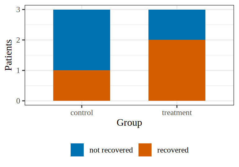
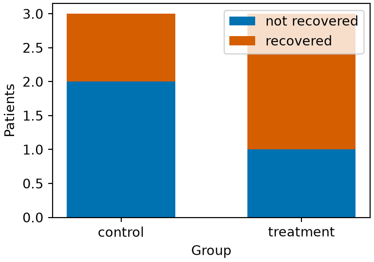
Figure 23: The six patients by group and recovery. Each group has three patients. One recovers in the control group, and two recover in the treatment group.
(a)
Stacked bar chart with two bars, control and treatment, each of height 3 patients. In the control bar, 1 patient recovered, in vermilion, and 2 did not, in blue. In the treatment bar, 2 patients recovered and 1 did not.
(b)
Stacked bar chart with two bars, control and treatment, each of height 3 patients. In the control bar, 1 patient recovered, in vermilion, and 2 did not, in blue. In the treatment bar, 2 patients recovered and 1 did not.

Solution 51. Order the patients control-first, and let the three control outcomes be \(y = 0, 0, 1\) and the three treatment outcomes \(y = 0, 1, 1\):

\[\design(\mx) = \begin{bmatrix} 1 & -1 \\ 1 & -1 \\ 1 & -1 \\ 1 & 1 \\ 1 & 1 \\ 1 & 1 \end{bmatrix}, \qquad \vy = \begin{bmatrix} 0 \\ 0 \\ 1 \\ 0 \\ 1 \\ 1\end{bmatrix}\]

Exercise 52 (A logistic regression you can fit by hand (part 1b))

Exercise 52 (A logistic regression you can fit by hand (part 1b)) Use the setup of Exercise 51.

Evaluate \(\grad_{\vcoef}\,\ell = \tp{\design(\mx)}\paren{\vy - \vprob}\) at \(\vcoef = \vzero\).

Solution 52. This continues Solution 51.

At \(\vcoef = \vzero\), every \(\prob_i = \sigmoid(0)\), which is \(1/2\), so \(\vy - \vprob = \pt{-\tfrac12, -\tfrac12, \tfrac12, -\tfrac12, \tfrac12, \tfrac12}\).

The intercept component of \(\tp{\design(\mx)}\paren{\vy - \vprob}\) is the sum of the entries of \(\vy - \vprob\):

\[ \begin{aligned} \sumin (y_i - \prob_i) &= \sumin y_i - \sumin \prob_i && \text{(split the sum)} \\ &= 3 - 6 \times \tfrac12 && \text{(three recoveries, six probabilities of } \tfrac12\text{)} \\ &= 0. \end{aligned} \]

The slope component multiplies each entry by \(x_i\) before summing:

\[ \begin{aligned} \sumin x_i(y_i - \prob_i) &= -\paren{-\tfrac12 - \tfrac12 + \tfrac12} + \paren{-\tfrac12 + \tfrac12 + \tfrac12} && \text{(control rows, then treatment rows)} \\ &= -\paren{-\tfrac12} + \tfrac12 && \text{(add within each group)} \\ &= 1. \end{aligned} \]

Exercise 53 (A logistic regression you can fit by hand (part 1c))

Exercise 53 (A logistic regression you can fit by hand (part 1c)) Use the setup of Exercise 51.

Interpret each of the two components of the gradient of Exercise 52.

Solution 53. This continues Solution 51 and Solution 52.

Three of the six patients recovered, and the probabilities at \(\vcoef = \vzero\) also sum to three, so the starting point is already calibrated in aggregate, in the sense of Solution 40.

The slope component is positive: the group coded \(+1\) has more recoveries than the probabilities at \(\vcoef = \vzero\) predict, and the group coded \(-1\) has fewer. Increasing \(\coef{1}\) from \(0\) therefore increases the log-likelihood \(\llik\).

Exercise 54 (A logistic regression you can fit by hand (part 2))

Exercise 54 (A logistic regression you can fit by hand (part 2)) Use the setup of Exercise 51.

Give the total log loss at \(\vcoef = \vzero\), exactly and to four significant figures. Why is this the value for any dataset of six observations at \(\vcoef = \vzero\)?

Solution 54. Every \(\prob_i = 1/2\), so every observation contributes \(-\log \tfrac12\), which equals \(\log 2\), whatever its label. The total log loss at \(\vcoef = \vzero\) is therefore

\[ -\llik(\vzero) = 6\log 2, \]

which is 4.159 to four significant figures.

The value does not depend on the data. At \(\vcoef = \vzero\) the model predicts \(1/2\) for every observation, so it scores \(\log 2\) per observation whatever the outcomes are, and the total for \(n\) observations is \(n \log 2\). That makes \(n\log 2\) a reference point: the coefficients \(\vcoef = \vzero\) attain it without using the data, and the fitted model’s improvement can be measured against it.

Exercise 55 (A logistic regression you can fit by hand (part 3))

Exercise 55 (A logistic regression you can fit by hand (part 3)) Use the setup of Exercise 51.

Use the symmetry of the design and the intercept score equation to show that \(\hcoef{0} = 0\).

Solution 55. In the trial of Exercise 51, the control and treatment groups have the same size, and their codes \(x = \pm 1\) are negatives of each other. Let \(\prob_+ = \sigmoid(\coef{0} + \coef{1})\) be the probability for the treatment group and \(\prob_- = \sigmoid(\coef{0} - \coef{1})\) the probability for the control group.

The intercept score equation \(\sum_i \prob_i = \sum_i y_i\) is

\[ \begin{aligned} 3\prob_- + 3\prob_+ &= 1 + 2 && \text{(three patients per group; one and two recoveries)} \\ 3\prob_- + 3\prob_+ &= 3 && \text{(add)} \\ \prob_- + \prob_+ &= 1 && \text{(divide by } 3\text{)}. \end{aligned} \]

By part 2 of the sigmoid properties exercise, \(1 - \prob_+ = \sigmoid(-\coef{0} - \coef{1})\), so the last equation is equivalent to \(\sigmoid(\coef{0} - \coef{1}) = \sigmoid(-\coef{0} - \coef{1})\). The logistic function is strictly increasing, so its arguments are equal:

\[ \begin{aligned} \coef{0} - \coef{1} &= -\coef{0} - \coef{1} && \text{(equal arguments)} \\ 2\coef{0} - \coef{1} &= -\coef{1} && \text{(add } \coef{0}\text{)} \\ 2\coef{0} &= 0 && \text{(add } \coef{1}\text{)} \\ \coef{0} &= 0 && \text{(divide by } 2\text{)}. \end{aligned} \]

So \(\hcoef{0} = 0\), and \(\prob_- = 1 - \prob_+\).

Theorem 15 (The intercept of a balanced two-group fit)

Theorem 15 (The intercept of a balanced two-group fit) Let two groups of \(n\) patients each be coded \(x = -1\) and \(x = +1\), with \(n\) recoveries altogether. Fit \(\condPr{\Outvar = 1}{x} = \sigmoid(\coef{0} + \coef{1} x)\) by maximum likelihood, and write \(\prob_- = \sigmoid(\coef{0} - \coef{1})\) and \(\prob_+ = \sigmoid(\coef{0} + \coef{1})\) for the fitted probabilities of the two groups. Every solution of the score equations has \(\hcoef{0} = 0\), and then \(\prob_- = 1 - \prob_+\).

Proof

Proof. The intercept score equation \(\sum_i \prob_i = \sum_i y_i\) reads \(n\prob_- + n\prob_+ = n\), so

\[ \sigmoid(\coef{0} - \coef{1}) = \prob_- = 1 - \prob_+ = \sigmoid(-\coef{0} - \coef{1}), \]

by the symmetry of the logistic function. The logistic function is strictly increasing, so \(\coef{0} - \coef{1} = -\coef{0} - \coef{1}\), which gives \(\coef{0} = 0\).

Exercise 56 (A logistic regression you can fit by hand (part 3b))

Exercise 56 (A logistic regression you can fit by hand (part 3b)) Use the setup of Exercise 51.

Use the score equation for \(\coef{1}\) and the result of Exercise 55 to find \(\hcoef{1}\) exactly.

Solution 56. This continues Solution 55.

With \(\hcoef{0} = 0\) and \(\prob_- = 1 - \prob_+\) from Solution 55, the slope score equation \(\sumin x_i\paren{y_i - \prob_i} = 0\) is

\[ \begin{aligned} -\paren{1 - 3\prob_-} + \paren{2 - 3\prob_+} &= 0 && \text{(control rows have } x = -1\text{, treatment rows } x = 1\text{)} \\ -1 + 3\prob_- + 2 - 3\prob_+ &= 0 && \text{(remove the parentheses)} \\ 1 + 3\prob_- - 3\prob_+ &= 0 && \text{(}-1 + 2 = 1\text{)} \\ 1 + 3\paren{1 - \prob_+} - 3\prob_+ &= 0 && \text{(}\prob_- = 1 - \prob_+\text{)} \\ 1 + 3 - 3\prob_+ - 3\prob_+ &= 0 && \text{(distribute } 3\text{)} \\ 4 - 6\prob_+ &= 0 && \text{(collect terms)} \\ \prob_+ &= \tfrac{2}{3} && \text{(solve for } \prob_+\text{)}. \end{aligned} \]

Then \(\prob_- = \tfrac13\). Because \(\hcoef{0} = 0\), \(\prob_+ = \sigmoid(\hcoef{1})\), and

\[ \begin{aligned} \hcoef{1} &= \logit\paren{\tfrac{2}{3}} && \text{(invert } \sigmoid\text{)} \\ &= \log\frac{2/3}{1/3} && \text{(definition of } \logit\text{)} \\ &= \log 2 && \text{(simplify the fraction)}, \end{aligned} \]

which is 0.6931.

Exercise 57 (A logistic regression you can fit by hand (part 4))

Exercise 57 (A logistic regression you can fit by hand (part 4)) Use the setup of Exercise 51.

Give the fitted probabilities.

Solution 57. The fitted probability vector is \(\hat{\vprob} = \paren{\tfrac13, \tfrac13, \tfrac13, \tfrac23, \tfrac23, \tfrac23}\).

Exercise 58 (A logistic regression you can fit by hand (part 4b))

Exercise 58 (A logistic regression you can fit by hand (part 4b)) Use the setup of Exercise 51.

Verify both score equations at the fitted probabilities of Exercise 57.

Solution 58. This continues Solution 57.

At the fitted probabilities of Solution 57, for the intercept equation,

\[ \begin{aligned} \sumin \prob_i &= 3 \times \tfrac13 + 3 \times \tfrac23 \\ &= 1 + 2 \\ &= 3, \end{aligned} \]

which equals \(\sumin \outvar_i\).

For the slope equation,

\[ \begin{aligned} \sumin \predvar_i \prob_i &= -3 \times \tfrac13 + 3 \times \tfrac23 \\ &= -1 + 2 \\ &= 1, \end{aligned} \]

and \(\sumin \predvar_i \outvar_i = -1 + 2\), which is also \(1\), so their difference is zero.

Here \(\prob_- = 1/3\) equals the proportion of recoveries in the control group (\(1\) of \(3\)), and \(\prob_+ = 2/3\) equals the proportion in the treatment group (\(2\) of \(3\)): the fitted probabilities equal the observed group proportions. With one binary predictor and an intercept, the two score equations make the fitted probabilities sum to the observed count in each group. The model has two parameters and the data have two groups, so the model can match both group proportions exactly, and it does.

Exercise 59 (A logistic regression you can fit by hand (part 5))

Exercise 59 (A logistic regression you can fit by hand (part 5)) Use the setup of Exercise 51.

The treatment group’s odds of recovery are \(2:1\) and the control group’s are \(1:2\), so the odds ratio between the groups is \(4\). But \(\e{\hcoef{1}} = 2\). Explain the difference between \(\e{\hcoef{1}}\) and the odds ratio.

Solution 59. The slope \(\coef{1}\) is the change in log-odds per one-unit increase in \(\predvar\), and under the coding \(\predvar \in \{-1, +1\}\) the two groups are two units apart. The treatment-versus-control odds ratio is therefore

\[ \begin{aligned} \e{2\hcoef{1}} &= \e{2\log 2} && \text{(}\hcoef{1} = \log 2\text{)} \\ &= \paren{\e{\log 2}}^2 && \text{(power of a power)} \\ &= 2^2 && \text{(}\e{\log a} = a\text{)} \\ &= 4, \end{aligned} \]

whereas \(\e{\hcoef{1}} = 2\) is the odds ratio for a one-unit increase, from \(x = -1\) to \(x = 0\) or from \(x = 0\) to \(x = +1\).

Exercise 60 (A logistic regression you can fit by hand (part 5b))

Exercise 60 (A logistic regression you can fit by hand (part 5b)) Use the setup of Exercise 51.

State what \(\hcoef{1}\) would have been under the coding \(\predvar \in \{0, 1\}\).

Solution 60. This continues Solution 59.

Under the indicator coding \(x \in \{0, 1\}\), the two groups are one unit apart, so \(\hcoef{1} = \log 4\), which is 1.386, and \(\e{\hcoef{1}} = 4\) is the between-group odds ratio itself. The intercept changes to \(\logit(1/3) = -\log 2\), so that the fitted probability for the control group (\(\predvar = 0\)) is still \(1/3\).

The fitted probabilities are the same under this coding and under the \(\pm 1\) coding of Solution 59; only the parameterization differs. Coding a two-level predictor as a \(\{0,1\}\) indicator makes \(\e{\hcoef{1}}\) equal to the between-group odds ratio.

Exercise 61 (A logistic regression you can fit by hand (part 6))

Exercise 61 (A logistic regression you can fit by hand (part 6)) Use the setup of Exercise 51.

Give the total log loss at \(\hvcoef\).

Solution 61. Four observations have outcomes equal to the majority outcome in their group, the two treated patients who recovered and the two control patients who did not, and each contributes \(-\log\tfrac23\), which equals \(\log\tfrac32\). The other two observations each contribute \(-\log\tfrac13\), which equals \(\log 3\):

\[ \begin{aligned} -\llikf{\hvcoef} &= 4\log\tfrac32 + 2\log 3 && \text{(sum the contributions)} \\ &= 4\log 3 - 4\log 2 + 2\log 3 && \text{(log of a quotient)} \\ &= 6\log 3 - 4\log 2 && \text{(collect the } \log 3 \text{ terms)}, \end{aligned} \]

which is 3.819.

Exercise 62 (A logistic regression you can fit by hand (part 6b))

Exercise 62 (A logistic regression you can fit by hand (part 6b)) Use the setup of Exercise 51.

Use the drop in total log loss from Exercise 54 (at \(\vcoef = \vzero\)) to Exercise 61 (at \(\hvcoef\)) to test \(H_0: \coef{1} = 0\) with a likelihood ratio test.

Solution 62. This continues Solution 61.

The decrease in negative log-likelihood from Solution 54 is

\[ \begin{aligned} 6\log 2 - \paren{6\log 3 - 4\log 2} &= 6\log 2 - 6\log 3 + 4\log 2 && \text{(remove the parentheses)} \\ &= 10\log 2 - 6\log 3 && \text{(collect the } \log 2 \text{ terms)}, \end{aligned} \]

which is 0.3398, so the likelihood ratio between the fitted model and the model with \(\coef{1} = 0\) is \(\e{0.3398}\), which is 1.405. The fitted model with \(\coef{1} = 0\) has \(\hcoef{0} = \logit(3/6)\), which is \(0\), so its negative log-likelihood is the \(6 \log 2\) of Solution 54.

The likelihood ratio test statistic is twice the change in log-likelihood, \(G^2 = 2 \times 0.3398\), which is 0.6796. Against the chi-square distribution \(\chi^2_1\), it gives \(p = 0.41\).

Exercise 63 (A logistic regression you can fit by hand (part 6c))

Exercise 63 (A logistic regression you can fit by hand (part 6c)) Use the setup of Exercise 51.

Explain what the result of the test of Exercise 62 implies for the trial.

Solution 63. This continues Solution 61.

The test of Solution 62 shows that the six-patient trial gives very little evidence against the null hypothesis \(\coef{1} = 0\). A fourfold odds ratio (\(\e{2\hcoef{1}} = 4\)) is a large point estimate, but six observations are too few to distinguish it from chance variation. The estimate \(\hcoef{1} = \log 2\) has a standard error of \(\sqrt{3}/2\), which is 0.866, larger than the estimate itself. That standard error comes from the observed information matrix. Every observation has \(W_{ii} = \tfrac13 \times \tfrac23\), which is \(\tfrac29\), and \(\stprod{\design(\mx)} = 6I\), so

\[ \begin{aligned} \tp{\design(\mx)} W \design(\mx) &= \tfrac{2}{9}\stprod{\design(\mx)} && \text{(}W = \tfrac29 I\text{)} \\ &= \tfrac{2}{9} \cdot 6I && \text{(}\stprod{\design(\mx)} = 6I\text{)} \\ &= \tfrac{4}{3}I, \end{aligned} \]

and the standard error of \(\hcoef{1}\) is \(\sqrt{\paren{\tfrac43}^{-1}}\), which equals \(\sqrt{3}/2\).

Exercise 64 (Choosing the step size for the fit you just did by hand)

Exercise 64 (Choosing the step size for the fit you just did by hand) The fit of Exercise 51 has an exact solution, \(\hvcoef = (0, \log 2)\) (Exercise 55 and Exercise 56), so the exact error of gradient ascent can be computed at every step. Run gradient ascent on the log-likelihood,

\[\iterpoint{\vcoef}{\iter+1} = \iterpoint{\vcoef}{\iter} + \learnrate\,\tp{\design(\mx)}\devof{\vy}{\iterpoint{\vprob}{\iter}},\]

starting from \(\iterpoint{\vcoef}{0} = \vzero\).

Show that \(\coef{0}\) stays at \(0\) for every step, whatever \(\learnrate\) is, so that the iteration changes only \(\coef{1}\).

Solution 64. The intercept column of \(\design(\mx)\) is all ones, so \(\sum_i (y_i - \prob_i)\) is the first component of the gradient. Suppose \(\coef{0} = 0\) at some step. Then \(z_i = \coef{1} x_i\), so the three controls all have \(\prob = \sigmoid(-\coef{1})\), and the three treated patients all have \(\prob = \sigmoid(\coef{1})\). By part 2 of the sigmoid properties exercise, \(\sigmoid(-\coef{1}) + \sigmoid(\coef{1}) = 1\), so

\[ \begin{aligned} \sum_i \prob_i &= 3\sigmoid(-\coef{1}) + 3\sigmoid(\coef{1}) && \text{(three patients per group)} \\ &= 3\sb{\sigmoid(-\coef{1}) + \sigmoid(\coef{1})} && \text{(factor out } 3\text{)} \\ &= 3 && \text{(}\sigmoid(-a) + \sigmoid(a) = 1\text{)}, \end{aligned} \]

which equals \(\sum_i y_i\), the three recoveries. The first component of the gradient is therefore zero, and the step does not change the intercept. The intercept starts at \(0\), so it stays at \(0\) for every step and every \(\learnrate\).

Exercise 55 used the same symmetry to show that \(\hcoef{0} = 0\); here it applies at every step, not only at the maximizer.

Exercise 65 (Choosing the step size for the fit you just did by hand (part 2))

Exercise 65 (Choosing the step size for the fit you just did by hand (part 2)) Use the setup of Exercise 64.

Show that the remaining component of the gradient satisfies

\[g(\coef{1}) = 4 - 6\,\sigmoid(\coef{1}).\]

Solution 65. In the iteration of Exercise 64, the slope component of the gradient has the form \(g(\coef{1}) = \sum_i x_i (y_i - \prob_i)\). With \(\coef{0} = 0\), the controls have \(x_i = -1\) and \(\prob_i = \sigmoid(-\coef{1})\), and the treated patients have \(x_i = 1\) and \(\prob_i = \sigmoid(\coef{1})\), so

\[ \begin{aligned} g(\coef{1}) &= -\sb{1 - 3\sigmoid(-\coef{1})} + \sb{2 - 3\sigmoid(\coef{1})} && \text{(sum each group)} \\ &= -1 + 3\sigmoid(-\coef{1}) + 2 - 3\sigmoid(\coef{1}) && \text{(remove the brackets)} \\ &= 1 + 3\sigmoid(-\coef{1}) - 3\sigmoid(\coef{1}) && \text{(}-1 + 2 = 1\text{)} \\ &= 1 + 3\sb{1 - \sigmoid(\coef{1})} - 3\sigmoid(\coef{1}) && \text{(}\sigmoid(-a) = 1 - \sigmoid(a)\text{)} \\ &= 1 + 3 - 3\sigmoid(\coef{1}) - 3\sigmoid(\coef{1}) && \text{(distribute } 3\text{)} \\ &= 4 - 6\,\sigmoid(\coef{1}) && \text{(collect terms)}. \end{aligned} \]

Exercise 66 (Choosing the step size for the fit you just did by hand (part 3))

Exercise 66 (Choosing the step size for the fit you just did by hand (part 3)) Use the setup of Exercise 64.

Check \(g(0)\) against the value that Exercise 52 found at \(\vcoef = \vzero\).

Solution 66. At \(\coef{1} = 0\),

\[ \begin{aligned} g(0) &= 4 - 6 \cdot \tfrac12 && \text{(}\sigmoid(0) = \tfrac12\text{)} \\ &= 1, \end{aligned} \]

which is the slope component that Solution 52 found.

Exercise 67 (Choosing the step size for the fit you just did by hand (part 3b))

Exercise 67 (Choosing the step size for the fit you just did by hand (part 3b)) Use the setup of Exercise 64.

Check \(g(\log 2)\) against the score equation of Exercise 56.

Solution 67. This continues Solution 66.

At \(\coef{1} = \log 2\),

\[ \begin{aligned} g(\log 2) &= 4 - 6 \cdot \tfrac23 && \text{(}\sigmoid(\log 2) = \tfrac23\text{)} \\ &= 0, \end{aligned} \]

which agrees with the slope score equation of Solution 56. The whole run is the one-variable iteration \(\coef{1} \leftarrow \coef{1} + \learnrate\sb{4 - 6\sigmoid(\coef{1})}\).

Exercise 68 (Choosing the step size for the fit you just did by hand (part 4))

Exercise 68 (Choosing the step size for the fit you just did by hand (part 4)) Use the setup of Exercise 64.

Let \(\learnrate = \tfrac12\), and give \(\coef{1}\) after each of five steps, to six decimal places. Tabulate the error \(\coef{1} - \log 2\) alongside, and the ratio of each error to the one before it. What value does that ratio approach?

Solution 68. With \(\learnrate = \tfrac12\):

Show code
# the one-variable iteration beta_1 <- beta_1 + rate * (4 - 6 * sigmoid(beta_1))
ascent_steps <- function(rate, steps, start = 0) {
  b <- numeric(steps)
  current <- start
  for (t in seq_len(steps)) {
    current <- current + rate * (4 - 6 * plogis(current))
    b[t] <- current
  }
  b
}
half_b <- ascent_steps(rate = 1 / 2, steps = 5)
half_err <- half_b - log(2)
knitr::kable(
  data.frame(
    step = 1:5,
    b = sprintf("%.6f", half_b),
    err = sprintf("%.6f", half_err),
    ratio = c("---", sprintf("%.4f", half_err[-1] / half_err[-5]))
  ),
  col.names = c(
    "step", "$\\coef{1}$", "$\\coef{1} - \\log 2$", "ratio to previous"
  )
)
step \(\coef{1}\) \(\coef{1} - \log 2\) ratio to previous
1 0.500000 -0.193147 —
2 0.632622 -0.060525 0.3134
3 0.673371 -0.019776 0.3267
4 0.686598 -0.006549 0.3312
5 0.690969 -0.002178 0.3326
Show code
import numpy as np
from scipy.special import expit

def ascent_steps(rate, steps, start=0.0):
    b, current = [], start
    for _ in range(steps):
        current = current + rate * (4 - 6 * expit(current))
        b.append(current)
    return np.array(b)

half_b = ascent_steps(0.5, 5)
half_err = half_b - np.log(2)
for t in range(5):
    ratio = "---" if t == 0 else f"{half_err[t] / half_err[t - 1]:.4f}"
    print(f"{t + 1}  {half_b[t]:.6f}  {half_err[t]:.6f}  {ratio}")
1  0.500000  -0.193147  ---
2  0.632622  -0.060525  0.3134
3  0.673371  -0.019776  0.3267
4  0.686598  -0.006549  0.3312
5  0.690969  -0.002178  0.3326

Every error is negative, so every iterate is below \(\log 2\), which is 0.693147, and the error shrinks by a factor that approaches \(1/3\).

Exercise 69 (Choosing the step size for the fit you just did by hand (part 5))

Exercise 69 (Choosing the step size for the fit you just did by hand (part 5)) Use the setup of Exercise 64.

Now let \(\learnrate = 2\), and give \(\coef{1}\) after each of five steps.

Solution 69.

Show code
two_b <- ascent_steps(rate = 2, steps = 5)
sprintf("%.6f", two_b)
[1] "2.000000"  "-0.569565" "3.094388"  "-0.385540" "2.756962" 

With \(\learnrate = 2\), the five iterates are \(2.000000\), \(-0.569565\), \(3.094388\), \(-0.385540\), \(2.756962\). They alternate between values below and above \(\log 2\), and they do not approach it.

Exercise 70 (Choosing the step size for the fit you just did by hand (part 6))

Exercise 70 (Choosing the step size for the fit you just did by hand (part 6)) Use the setup of Exercise 64.

Do the iterates grow without bound? Prove your answer, using the bound on \(\norm{\grad C_i}\) from Exercise 38.

Solution 70. With \(\learnrate = 2\), the iterates overshoot the maximizer at each step, but they stay bounded.

Exercise 38 bounds each observation’s gradient by \(\norm{\vx_i}\), and here that bound makes the one-variable gradient bounded. Because \(\sigmoid(\coef{1})\) is strictly between \(0\) and \(1\),

\[g(\coef{1}) = 4 - 6\sigmoid(\coef{1}) \in (-2, 4)\]

for every \(\coef{1} \in \reals\). A single step therefore changes \(\coef{1}\) by more than \(-2\learnrate\) and less than \(4\learnrate\), whatever the current value.

That bound keeps the iterates in a closed, bounded interval. Let \(K = [\log 2 - 2\learnrate,\; \log 2 + 4\learnrate]\), and consider any \(\coef{1} \in K\).

  • If \(\coef{1} \ge \log 2\), then \(\sigmoid(\coef{1}) \ge \tfrac23\), so \(g(\coef{1}) \le 0\), and the step moves \(\coef{1}\) down or not at all. The new value is at most \(\coef{1}\), which is at most \(\log 2 + 4\learnrate\), and more than \(\coef{1} - 2\learnrate\), which is at least \(\log 2 - 2\learnrate\).
  • If \(\coef{1} \le \log 2\), then \(g(\coef{1}) \ge 0\), and the step moves \(\coef{1}\) up or not at all. The new value is at least \(\coef{1}\), which is at least \(\log 2 - 2\learnrate\), and less than \(\coef{1} + 4\learnrate\), which is at most \(\log 2 + 4\learnrate\).

In both cases the next iterate is in \(K\).

The iteration starts at \(\coef{1} = 0\), which is in \(K\) whenever \(2\learnrate \ge \log 2\). For \(\learnrate = 2\), the sequence therefore stays in \([-3.307, 8.693]\) for every \(t\), and all five iterates of Solution 69 are in this interval.

Exercise 71 (Choosing the step size for the fit you just did by hand (part 7))

Exercise 71 (Choosing the step size for the fit you just did by hand (part 7)) Use the setup of Exercise 64.

Linearize the update map of Exercise 64 about \(\hcoef{1} = \log 2\) and find its derivative there.

Solution 71. Let the update map be \(T(\coef{1}) = \coef{1} + \learnrate\sb{4 - 6\sigmoid(\coef{1})}\). Its derivative is

\[ \begin{aligned} T'(\coef{1}) &= 1 - 6\learnrate\,\sigmoid'(\coef{1}) && \text{(differentiate term by term)} \\ &= 1 - 6\learnrate\,\sigmoid(\coef{1})\sb{1 - \sigmoid(\coef{1})} && \text{(}\sigmoid' = \sigmoid(1-\sigmoid)\text{)}. \end{aligned} \]

The second line uses the derivative of \(\sigmoid\) from part 3 of the sigmoid properties exercise.

At the fixed point \(\coef{1} = \log 2\), \(\sigmoid(\coef{1}) = \tfrac23\), so

\[ \begin{aligned} \sigmoid'(\log 2) &= \tfrac23 \cdot \tfrac13 \\ &= \tfrac29 \end{aligned} \]

and

\[ \begin{aligned} T'(\log 2) &= 1 - 6\learnrate \cdot \tfrac29 \\ &= 1 - \tfrac43 \learnrate. \end{aligned} \]

Near \(\log 2\), the linearized map is \(T(\coef{1}) \approx \log 2 + T'(\log 2)\paren{\coef{1} - \log 2}\), so each step multiplies the error \(\coef{1} - \log 2\) by about \(1 - \tfrac43 \learnrate\).

Exercise 72 (Choosing the step size for the fit you just did by hand (part 8))

Exercise 72 (Choosing the step size for the fit you just did by hand (part 8)) Use the setup of Exercise 64.

For which \(\learnrate\) does the iteration converge?

Solution 72. Near \(\log 2\), each step multiplies the error by about \(1 - \tfrac43 \learnrate\), so the iteration converges to \(\log 2\) from starting points near it when \(\abs{1 - \tfrac43 \learnrate} < 1\). That inequality holds when

\[0 < \learnrate < \tfrac32.\]

Exercise 73 (Choosing the step size for the fit you just did by hand (part 9))

Exercise 73 (Choosing the step size for the fit you just did by hand (part 9)) Use the setup of Exercise 64.

Check that your answer accounts for both Exercise 68 and Exercise 69.

Solution 73. Both earlier parts follow from the multiplier \(1 - \tfrac43 \learnrate\).

  • At \(\learnrate = \tfrac12\), the multiplier is \(1 - \tfrac23\), which is \(\tfrac13\). It is positive, so the error keeps its sign, and it equals the ratio \(1/3\) that the errors approach in Solution 68.
  • At \(\learnrate = 2\), the multiplier is \(1 - \tfrac83\), which is \(-\tfrac53\). It is negative, so the error changes sign at every step, and its absolute value is greater than \(1\), so iterates near \(\log 2\) move away from it.

With Solution 70, this result determines the behavior at \(\learnrate = 2\): the sequence does not converge to \(\log 2\), and it does not leave the interval \(K\).

Exercise 74 (Choosing the step size for the fit you just did by hand (part 10))

Exercise 74 (Choosing the step size for the fit you just did by hand (part 10)) Use the setup of Exercise 64.

The step-size condition of Corollary 1 is \(\learnrate < 8 / \eigval_{\max}(\tp{\design(\mx)} \design(\mx))\). Evaluate it here.

Solution 74. The columns of \(\design(\mx)\) are the intercept column of ones and the \(\predvar\) column \((-1,-1,-1,+1,+1,+1)\). These two columns are orthogonal, and each has squared length \(6\), so

\[\stprod{\design(\mx)} = \begin{pmatrix} 6 & 0 \\ 0 & 6 \end{pmatrix}, \qquad \eigval_{\max}\paren{\stprod{\design(\mx)}} = 6,\]

and the bound gives \(\learnrate < 8/6\), which is \(4/3\).

Exercise 75 (Choosing the step size for the fit you just did by hand (part 10b))

Exercise 75 (Choosing the step size for the fit you just did by hand (part 10b)) Use the setup of Exercise 64.

Compare the bound of Exercise 74 with the exact threshold from Exercise 72.

Solution 75. This continues Solution 74.

The bound of Solution 74 is \(4/3\), and the exact threshold of Solution 72 is \(3/2\), so the bound is smaller than the threshold by a factor of \(\tfrac{3}{2} \div \tfrac{4}{3}\), which is \(\tfrac98\).

Exercise 76 (Choosing the step size for the fit you just did by hand (part 10c))

Exercise 76 (Choosing the step size for the fit you just did by hand (part 10c)) Use the setup of Exercise 64.

Explain the difference between the bound of Exercise 74 and the exact threshold from Exercise 72.

Solution 76. This continues Solution 74.

The difference between the bound and the exact threshold (Solution 75) comes from the inequality \(W_{ii} \le 1/4\). Equality holds only where \(\prob_i = 1/2\), but at the maximum likelihood estimate the fitted probabilities are \(1/3\) and \(2/3\), so every \(W_{ii}\) is \(\tfrac13 \cdot \tfrac23\), which is \(\tfrac29\). The Hessian at the maximum is therefore \(\tfrac29 \stprod{\design(\mx)}\), which is \(\tfrac43 I\), rather than the bound \(\tfrac14 \stprod{\design(\mx)}\), which is \(\tfrac32 I\). For the Hessian at the maximum, \(2/\eigval_{\max}\) is \(3/2\), the exact threshold. The ratio \(\tfrac98\) equals \(\tfrac14 \div \tfrac29\).

The bound holds for every \(\vcoef\), and it is smaller than the exact threshold by the factor by which \(\prob_i(1 - \prob_i)\) at the maximum is below \(1/4\). A fit that separates the classes well has fitted probabilities near \(0\) and \(1\), so it has small curvature at the maximum and a larger stable step size.

Exercise 77 (Choosing the step size for the fit you just did by hand (part 11))

Exercise 77 (Choosing the step size for the fit you just did by hand (part 11)) Use the setup of Exercise 64.

Run the iteration with \(\learnrate = 2\) for a few thousand steps.

Solution 77.

Show code
long_two <- ascent_steps(rate = 2, steps = 4000)
last_two <- tail(long_two, 2)
cycle_two <- sort(last_two)
cycle_two
[1] -0.4689554  2.9126825

The last two values of \(\coef{1}\) after \(4000\) steps are -0.468955 and 2.912682.

Exercise 78 (Choosing the step size for the fit you just did by hand (part 11b))

Exercise 78 (Choosing the step size for the fit you just did by hand (part 11b)) Use the setup of Exercise 64.

Describe the behavior of \(\coef{1}\) after many steps of the iteration of Exercise 77.

Solution 78. This continues Solution 77.

For \(\learnrate = 2\), the iterates approach a cycle of period \(2\), a pair of points that the update map \(T\) sends to each other. The sequence does not converge to a single point, and it does not grow without bound.

The two points of the cycle are on either side of \(\log 2\), where the update map \(T\) has its fixed point. The multiplier of Solution 71 at that fixed point is \(1 - \tfrac43 \learnrate\), which equals \(-\tfrac53\) for \(\learnrate = 2\). That is below \(-1\), so the iterates leave the fixed point.

Figure 24 plots the iterates for \(\learnrate = 2\) and, for comparison, for \(\learnrate = \tfrac12\).

Show code
asp_n <- 21
asp_steps <- seq_len(asp_n) - 1
asp_half <- numeric(asp_n)
asp_two <- numeric(asp_n)
for (asp_i in 2:asp_n) {
  asp_prev <- asp_half[asp_i - 1]
  asp_grad <- 4 - 6 * plogis(asp_prev)
  asp_half[asp_i] <- asp_prev + 0.5 * asp_grad
  asp_prev2 <- asp_two[asp_i - 1]
  asp_grad2 <- 4 - 6 * plogis(asp_prev2)
  asp_two[asp_i] <- asp_prev2 + 2 * asp_grad2
}
asp_names <- c("step size 1/2", "step size 2")
asp_step <- rep(asp_steps, 2)
asp_value <- c(asp_half, asp_two)
asp_rate <- rep(asp_names, each = asp_n)
asp_curves <- tibble::tibble(
  step = asp_step,
  value = asp_value,
  rate = asp_rate
)
asp_colours <- c("step size 1/2" = "#0072B2", "step size 2" = "#D55E00")
asp_types <- c("step size 1/2" = "solid", "step size 2" = "dashed")
asp_shapes <- c("step size 1/2" = 16, "step size 2" = 17)
asp_target <- log(2)
asp_curves |>
  ggplot2::ggplot(ggplot2::aes(step, value, colour = rate)) +
  ggplot2::geom_hline(
    yintercept = asp_target,
    linetype = "dotted",
    colour = "grey50"
  ) +
  ggplot2::geom_line(ggplot2::aes(linetype = rate)) +
  ggplot2::geom_point(ggplot2::aes(shape = rate)) +
  ggplot2::scale_colour_manual(values = asp_colours) +
  ggplot2::scale_linetype_manual(values = asp_types) +
  ggplot2::scale_shape_manual(values = asp_shapes) +
  ggplot2::labs(
    x = "Step",
    y = "Slope coefficient",
    colour = NULL,
    linetype = NULL,
    shape = NULL
  )
Show code
import matplotlib.pyplot as plt
import numpy as np
from scipy.special import expit

steps_asp = np.arange(21)
half_asp = np.zeros(21)
two_asp = np.zeros(21)
for i in range(1, 21):
    half_asp[i] = half_asp[i - 1] + 0.5 * (4 - 6 * expit(half_asp[i - 1]))
    two_asp[i] = two_asp[i - 1] + 2 * (4 - 6 * expit(two_asp[i - 1]))

fig, ax = plt.subplots(figsize=(5, 3.5), layout="constrained")
ax.axhline(np.log(2), color="grey", linestyle=":");
ax.plot(steps_asp, half_asp, color="#0072B2", marker="o", label="step size 1/2");
ax.plot(steps_asp, two_asp, color="#D55E00", linestyle="--", marker="^",
        label="step size 2");
ax.set_xlabel("Step");
ax.set_ylabel("Slope coefficient");
fig.legend(loc="outside lower center", ncol=2, frameon=False);
plt.show()
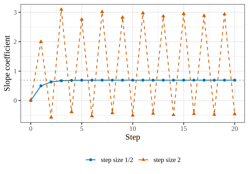
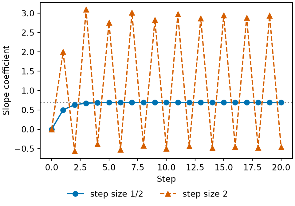
Figure 24: The iterates of \(\coef{1}\) for a step size of \(1/2\) and of \(2\), with the dotted line at \(\log 2\).
(a)
Line plot of the slope coefficient against the gradient ascent step, from step 0 to step 20. A dotted grey horizontal line marks log 2, about 0.69. A solid blue line with circles, for step size one half, rises from 0 at step 0 to 0.5 at step 1 and is within 0.01 of 0.69 from step 4 on. A dashed vermilion line with triangles, for step size 2, jumps from 0 to 2 at step 1 and then alternates between values near -0.5 and near 3, never settling.
(b)
Line plot of the slope coefficient against the gradient ascent step, from step 0 to step 20. A dotted grey horizontal line marks log 2, about 0.69. A solid blue line with circles, for step size one half, rises from 0 at step 0 to 0.5 at step 1 and is within 0.01 of 0.69 from step 4 on. A dashed vermilion line with triangles, for step size 2, jumps from 0 to 2 at step 1 and then alternates between values near -0.5 and near 3, never settling.

Exercise 79 (Choosing the step size for the fit you just did by hand (part 12))

Exercise 79 (Choosing the step size for the fit you just did by hand (part 12)) Use the setup of Exercise 64.

State what happens instead when the step size is too large for the least-squares cost, whose step-size bound the chapter on gradient descent derives.

Solution 79. Least squares behaves differently. Its objective is quadratic, so the update is linear, and each step multiplies the error component along an eigenvector by \(1 - 2\learnrate\eigval\), with no higher-order terms. When \(\abs{1 - 2\learnrate\eigval} > 1\) for some eigenvalue \(\eigval\), that component of the error is multiplied by the same factor at every step, so it grows geometrically and the iterates grow without bound.

In this one-variable logistic regression, the total log loss does not lead to this growth, for the reason shown in Solution 70. The fitted probabilities are in \((0, 1)\), so the gradient is bounded on \(\reals\), and a step size that is too large gives bounded iterates that do not converge, such as the cycle of period \(2\) at \(\learnrate = 2\). A step size that is too large therefore shows up differently in the two problems: the least-squares iterates grow until they overflow, and these logistic regression iterates stay bounded without converging. The bounded gradient bounds each step, not the iterates, so this argument does not carry over to every logistic regression: when the classes can be separated, the iterates grow without bound at any step size.

6 Newton’s method

Gradient ascent uses the first derivative of the log-likelihood, and needs a step size chosen by the user. Newton’s method also uses the second derivative, which sets both the direction and the length of each step. When the maximum likelihood estimate exists and the model has a modest number of coefficients, Newton’s method started at \(\vzero\) usually reaches the maximizer, up to rounding error, in a few iterations, and R’s glm() fits logistic regression with it.

Exercise 80 (Newton’s method, and why it is a weighted least squares fit)

Exercise 80 (Newton’s method, and why it is a weighted least squares fit) In Exercise 68, the error of gradient ascent shrank by a factor of about \(3\) per step, at a step size that had to be chosen. Newton’s method uses the second derivative of \(\llik\) as well as the first, and has no step size to choose.

Write the second-order Taylor expansion of \(\llik(\iterpoint{\vcoef}{\iter} + \vd)\) about the current iterate \(\iterpoint{\vcoef}{\iter}\), as a function of the step \(\vd\).

Solution 80. By Proposition 1, \(\llik = -C\), so Theorem 11 and Theorem 12 give the gradient and Hessian of \(\llik\):

\[ \grad \llik(\vcoef) = \tp{\design} \paren{\voutvar - \vprob}, \qquad \grad^2 \llik(\vcoef) = -\tp{\design} W \design. \]

Write \(\iterpoint{\vprob}{\iter}\) and \(\iterpoint{W}{\iter}\) for \(\vprob\) and \(W\) evaluated at \(\iterpoint{\vcoef}{\iter}\). Write \(q(\vd)\) for the second-order Taylor expansion of \(\llik\) about \(\iterpoint{\vcoef}{\iter}\):

\[ \llik(\iterpoint{\vcoef}{\iter} + \vd) \approx q(\vd) = \llik(\iterpoint{\vcoef}{\iter}) + \tp{\paren{\design \vd}} \devof{\voutvar}{\iterpoint{\vprob}{\iter}} - \tfrac12 \tp{\vd} \qform{\iterpoint{W}{\iter}}{\design} \vd . \]

Exercise 81 (Newton’s method, and why it is a weighted least squares fit (part 1b))

Exercise 81 (Newton’s method, and why it is a weighted least squares fit (part 1b)) Use the setup of Exercise 80.

Find the equation that the step \(\vd\) maximizing the expansion of Exercise 80 satisfies.

Solution 81. This continues Solution 80.

Let \(q\) be the expansion of Solution 80. By Theorem 12, the matrix \(\qform{\iterpoint{W}{\iter}}{\design}\) is positive semidefinite, so \(q\) is a concave quadratic in \(\vd\), and a step \(\vd\) maximizes \(q\) exactly when \(\grad q(\vd) = \vzero\):

\[ \begin{aligned} \grad q(\vd) &= \tp{\design} \devof{\voutvar}{\iterpoint{\vprob}{\iter}} - \qform{\iterpoint{W}{\iter}}{\design} \vd && \text{(differentiate each term of } q \text{)} \\ &= \vzero && \text{(stationarity)} \\ \Longrightarrow \quad \qform{\iterpoint{W}{\iter}}{\design} \vd &= \tp{\design} \devof{\voutvar}{\iterpoint{\vprob}{\iter}}. && \text{(move the second term to the right)} \end{aligned} \]

Exercise 82 (Newton’s method, and why it is a weighted least squares fit (part 2))

Exercise 82 (Newton’s method, and why it is a weighted least squares fit (part 2)) Use the setup of Exercise 80.

Assume that \(\design\) has full column rank. Show that the Newton update \(\iterpoint{\vcoef}{\iter+1} = \iterpoint{\vcoef}{\iter} + \vd\) is

\[ \iterpoint{\vcoef}{\iter+1} = \iterpoint{\vcoef}{\iter} + \inv{\qform{\iterpoint{W}{\iter}}{\design}} \tp{\design} \devof{\voutvar}{\iterpoint{\vprob}{\iter}}, \]

where \(\iterpoint{W}{\iter}\) is the weight matrix from Theorem 12 evaluated at \(\iterpoint{\vcoef}{\iter}\).

Solution 82. Every diagonal entry \(\prob_i \paren{1 - \prob_i}\) of \(\iterpoint{W}{\iter}\) is positive, so \(\tp{\vd} \qform{\iterpoint{W}{\iter}}{\design} \vd = \sumin \prob_i \paren{1 - \prob_i} \paren{\dprod{\vx_i}{\vd}}^2\) is \(0\) only when \(\design \vd = \vzero\), which for a full-column-rank \(\design\) requires \(\vd = \vzero\). So \(\qform{\iterpoint{W}{\iter}}{\design}\) is positive definite and invertible. Multiplying the equation of Solution 81 on the left by its inverse gives

\[ \vd = \inv{\qform{\iterpoint{W}{\iter}}{\design}} \tp{\design} \devof{\voutvar}{\iterpoint{\vprob}{\iter}}, \]

and adding \(\vd\) to \(\iterpoint{\vcoef}{\iter}\) gives the stated update.

Theorem 16 (The logistic log-likelihood is strictly concave)

Theorem 16 (The logistic log-likelihood is strictly concave) Let \(\llik = -C\) be the log-likelihood, the negative of the total log loss \(C\), and let \(W\) be the diagonal matrix of Theorem 12. If the design matrix \(\design\) has full column rank, then \(\grad^2 \llik(\vcoef) = -\tp{\design} W \design\) is negative definite for every \(\vcoef\). So \(\llik\) is strictly concave, and has at most one maximizer.

Proof

Proof. For any \(\vd \ne \vzero\), the diagonal entries \(\prob_i \paren{1 - \prob_i}\) of \(W\) are positive, so

\[ \begin{aligned} \tp{\vd} \tp{\design} W \design \vd &= \sumin \prob_i \paren{1 - \prob_i} \paren{\dprod{\vx_i}{\vd}}^2 && \text{(expand the quadratic form)} \\ &> 0. && \text{(} \design \vd \ne \vzero \text{ for a full-column-rank } \design \text{)} \end{aligned} \]

So \(\tp{\design} W \design\) is positive definite, and the Hessian \(-\tp{\design} W \design\) of \(\llik\) (Theorem 12) is negative definite. Then \(-\llik\) is strictly convex by the second-derivative test, and so has at most one global minimizer.

Example 27 (The six-patient study is strictly concave)

Example 27 (The six-patient study is strictly concave) In Exercise 51, the columns of \(\design\) are the ones vector and \(\vx = \tp{(-1, -1, -1, 1, 1, 1)}\). They are orthogonal, each with squared length \(6\), so \(\design\) has full column rank. At \(\vcoef = \vzero\), every \(\prob_i = \tfrac12\), so \(W = \tfrac14 \idmat\) and

\[ \begin{aligned} \grad^2 \llik(\vzero) &= -\tfrac14 \tp{\design} \design \\ &= -\tfrac32 \idmat, \end{aligned} \]

which is negative definite. At any other \(\vcoef\), the entries of \(W\) change, but by Theorem 16 the Hessian stays negative definite.

Figure 25 plots the function.

Show code
llc_x <- c(-1, -1, -1, 1, 1, 1)
llc_y <- c(1, 0, 0, 1, 1, 0)
llc_patients <- tibble::tibble(x = llc_x, y = llc_y)
llc_b0 <- seq(-2, 2, length.out = 121)
llc_b1 <- seq(-1, 2, length.out = 121)
llc_grid <- tidyr::expand_grid(b0 = llc_b0, b1 = llc_b1, llc_patients)
llc_terms <- llc_grid |>
  dplyr::mutate(z = b0 + b1 * x, ez = exp(z), term = y * z - log1p(ez))
llc_surface <- llc_terms |>
  dplyr::group_by(b0, b1) |>
  dplyr::summarise(llik = sum(term), .groups = "drop")
llc_where <- c("origin", "maximum")
llc_slope_max <- log(2)
llc_pts_b1 <- c(0, llc_slope_max)
llc_pts_b0 <- c(0, 0)
llc_pts <- tibble::tibble(b0 = llc_pts_b0, b1 = llc_pts_b1, where = llc_where)
llc_colours <- c(origin = "#D55E00", maximum = "#0072B2")
llc_shapes <- c(origin = 17, maximum = 16)
llc_surface |>
  ggplot2::ggplot(ggplot2::aes(b0, b1)) +
  ggplot2::geom_contour(ggplot2::aes(z = llik), colour = "grey50", bins = 12) +
  ggplot2::geom_point(
    data = llc_pts,
    ggplot2::aes(colour = where, shape = where),
    size = 3
  ) +
  ggplot2::scale_colour_manual(values = llc_colours) +
  ggplot2::scale_shape_manual(values = llc_shapes) +
  ggplot2::labs(x = "Intercept", y = "Slope", colour = NULL, shape = NULL)
Show code
import matplotlib.pyplot as plt
import numpy as np

x_llc = np.array([-1, -1, -1, 1, 1, 1])
y_llc = np.array([1, 0, 0, 1, 1, 0])
b0_llc, b1_llc = np.meshgrid(np.linspace(-2, 2, 121), np.linspace(-1, 2, 121))
z_llc = b0_llc[..., None] + b1_llc[..., None] * x_llc
llik_llc = (y_llc * z_llc - np.log1p(np.exp(z_llc))).sum(axis=-1)
fig, ax = plt.subplots(figsize=(6, 4), layout="constrained")
ax.contour(b0_llc, b1_llc, llik_llc, levels=12, colors="grey");
ax.plot(0, 0, color="#D55E00", marker="^", markersize=8, linestyle="", label="origin");
ax.plot(0, np.log(2), color="#0072B2", marker="o", markersize=8, linestyle="", label="maximum");
ax.set_xlabel("Intercept");
ax.set_ylabel("Slope");
ax.legend();
plt.show()
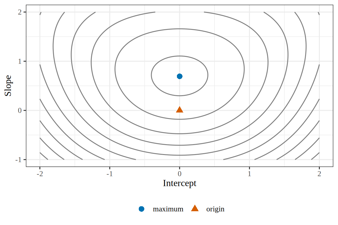
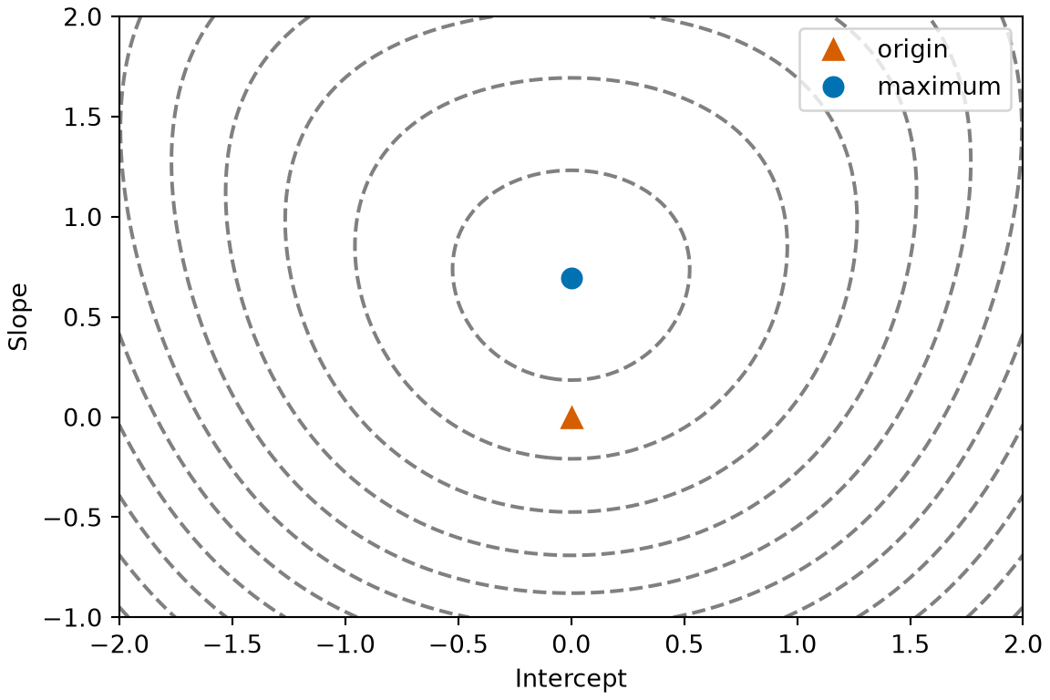
Figure 25: The log-likelihood of Exercise 51, drawn as nested curves around a single peak at the maximum (blue), as strict concavity requires.
(a)
Contour plot of the log-likelihood of the six-patient study over the intercept from -2 to 2 on the horizontal axis and the slope from -1 to 2 on the vertical axis. The contours are nested curves around a single peak. A vermilion triangle marks the origin and a blue circle marks the maximum at an intercept of 0 and a slope of 0.693.
(b)
Contour plot of the log-likelihood of the six-patient study over the intercept from -2 to 2 on the horizontal axis and the slope from -1 to 2 on the vertical axis. The contours are nested curves around a single peak. A vermilion triangle marks the origin and a blue circle marks the maximum at an intercept of 0 and a slope of 0.693.
Show code
llc3_x <- c(-1, -1, -1, 1, 1, 1)
llc3_y <- c(1, 0, 0, 1, 1, 0)
llc3_patients <- tibble::tibble(x = llc3_x, y = llc3_y)
# The grid holds the origin and the maximum, so both lie on the surface.
llc3_slope_max <- log(2)
llc3_b0 <- seq(-40, 40) / 20
llc3_b1_steps <- seq(-30, 60) / 30
llc3_b1_all <- c(llc3_b1_steps, llc3_slope_max)
llc3_b1 <- sort(llc3_b1_all)
llc3_n_b1 <- length(llc3_b1)
llc3_grid <- tidyr::expand_grid(b0 = llc3_b0, b1 = llc3_b1, llc3_patients)
llc3_terms <- llc3_grid |>
  dplyr::mutate(z = b0 + b1 * x, term = y * z - log1p(exp(z)))
llc3_surface <- llc3_terms |>
  dplyr::group_by(b0, b1) |>
  dplyr::summarise(llik = sum(term), .groups = "drop")
llc3_z <- matrix(llc3_surface$llik, nrow = llc3_n_b1)
llc3_at_zero <- dplyr::filter(llc3_surface, b0 == 0)
llc3_origin <- dplyr::filter(llc3_at_zero, b1 == 0)
llc3_peak <- dplyr::filter(llc3_at_zero, b1 == llc3_slope_max)
llc3_origin$z <- llc3_origin$llik
llc3_peak$z <- llc3_peak$llik
llc3_origin_marker <- list(color = "#D55E00", size = 6, symbol = "diamond")
llc3_peak_marker <- list(color = "#0072B2", size = 6)
llc3_stops <- c(0, 1)
llc3_cols <- c("#E5E5E5", "#808080")
llc3_scale <- list(llc3_stops, llc3_cols)
llc3_eye <- list(x = 1.7, y = -1.7, z = 0.9)
llc3_camera <- list(eye = llc3_eye)
llc3_xaxis <- list(title = "Intercept")
llc3_yaxis <- list(title = "Slope")
llc3_zaxis <- list(title = "Log-likelihood")
llc3_scene <- list(
  xaxis = llc3_xaxis,
  yaxis = llc3_yaxis,
  zaxis = llc3_zaxis,
  camera = llc3_camera
)
llc3_legend <- list(orientation = "h")
plotly::plot_ly() |>
  plotly::add_surface(
    x = llc3_b0,
    y = llc3_b1,
    z = llc3_z,
    colorscale = llc3_scale,
    showscale = FALSE,
    opacity = 0.7
  ) |>
  plotly::add_markers(
    data = llc3_origin,
    x = ~b0,
    y = ~b1,
    z = ~z,
    marker = llc3_origin_marker,
    name = "origin"
  ) |>
  plotly::add_markers(
    data = llc3_peak,
    x = ~b0,
    y = ~b1,
    z = ~z,
    marker = llc3_peak_marker,
    name = "maximum"
  ) |>
  plotly::layout(scene = llc3_scene, legend = llc3_legend)
Show code
import html
import numpy as np
import plotly.graph_objects as go

fig_alt = r.lsc_alt_sf

x_llc3 = np.array([-1, -1, -1, 1, 1, 1])
y_llc3 = np.array([1, 0, 0, 1, 1, 0])


def loglik_llc3(b0, b1):
    z = np.asarray(b0)[..., None] + np.asarray(b1)[..., None] * x_llc3
    return (y_llc3 * z - np.log1p(np.exp(z))).sum(axis=-1)


b0_axis_llc3 = np.linspace(-2, 2, 81)
b1_axis_llc3 = np.linspace(-1, 2, 81)
b0_llc3, b1_llc3 = np.meshgrid(b0_axis_llc3, b1_axis_llc3)
fig = go.Figure(data=[
    go.Surface(
        x=b0_axis_llc3, y=b1_axis_llc3, z=loglik_llc3(b0_llc3, b1_llc3),
        colorscale=[[0, "#E5E5E5"], [1, "#808080"]],
        showscale=False, opacity=0.4, showlegend=False,
    ),
    go.Scatter3d(
        x=[0], y=[0], z=[loglik_llc3(0, 0)], mode="markers",
        marker=dict(color="#D55E00", size=4, symbol="diamond"),
        name="origin",
    ),
    go.Scatter3d(
        x=[0], y=[np.log(2)], z=[loglik_llc3(0, np.log(2))], mode="markers",
        marker=dict(color="#0072B2", size=4, symbol="circle"),
        name="maximum",
    ),
])
fig.update_layout(
    scene=dict(
        xaxis_title="Intercept",
        yaxis_title="Slope",
        zaxis_title="Log-likelihood",
    ),
    legend=dict(orientation="h"),
);
print(
    "```{=html}\n"
    + f'<div role="group" aria-label="{html.escape(fig_alt)}">\n'
    + fig.to_html(full_html=False, include_plotlyjs="cdn")
    + "\n</div>\n```"
)
Figure 26: The log-likelihood of the six-patient study, as a surface over the intercept and slope. The surface is a single dome with one peak at the maximum (blue), as strict concavity requires. The origin (vermilion) is on the side of the dome.
(a)

Theorem 17 (The Newton update for logistic regression)

Theorem 17 (The Newton update for logistic regression) Let \(\iterpoint{\vprob}{\iter}\) and \(\iterpoint{W}{\iter}\) be the fitted probabilities and the weight matrix \(W\) from Theorem 12, evaluated at the current iterate \(\iterpoint{\vcoef}{\iter}\). If \(\design\) has full column rank, the Newton step from \(\iterpoint{\vcoef}{\iter}\) on the log-likelihood \(\llik\) is

\[ \iterpoint{\vcoef}{\iter+1} = \iterpoint{\vcoef}{\iter} + \inv{\qform{\iterpoint{W}{\iter}}{\design}} \tp{\design} \devof{\voutvar}{\iterpoint{\vprob}{\iter}}. \]

Proof

Proof. Maximizing \(\llik\) is minimizing \(C = -\llik\). By Theorem 11, \(\grad C(\iterpoint{\vcoef}{\iter}) = -\tp{\design} \devof{\voutvar}{\iterpoint{\vprob}{\iter}}\), and by Theorem 16, the Hessian \(\qform{\iterpoint{W}{\iter}}{\design}\) of \(C\) is positive definite, hence invertible. So the Newton step minimizing the quadratic model of \(C\) is

\[ \begin{aligned} -\inv{\qform{\iterpoint{W}{\iter}}{\design}} \grad C(\iterpoint{\vcoef}{\iter}) &= \inv{\qform{\iterpoint{W}{\iter}}{\design}} \tp{\design} \devof{\voutvar}{\iterpoint{\vprob}{\iter}}, \end{aligned} \]

and adding it to \(\iterpoint{\vcoef}{\iter}\) gives the update.

Exercise 83 (Newton’s method, and why it is a weighted least squares fit (part 3))

Exercise 83 (Newton’s method, and why it is a weighted least squares fit (part 3)) Use the setup of Exercise 80.

Compare the Newton update of Exercise 82 with the gradient ascent update of Exercise 64. Which quantity in the gradient ascent update has no counterpart in the Newton update?

Solution 83. The step size \(\learnrate\) has no counterpart. Gradient ascent moves in the direction of the gradient, and the step size \(\learnrate\), chosen separately, sets how far it moves; Exercise 64 studied that choice. Newton’s method moves straight to the maximizer of the quadratic expansion \(q\) of Solution 80, so the matrix \(\inv{\qform{\iterpoint{W}{\iter}}{\design}}\), computed from the curvature, sets both the direction and the length of the step, and nothing is left to choose. Far from the maximizer the quadratic expansion can be a poor guide, and a full Newton step can overshoot, so a damped Newton method shortens a step that makes the fit worse [11, Sec. 9.5].


Exercise 84 (Newton’s method, and why it is a weighted least squares fit (part 4))

Exercise 84 (Newton’s method, and why it is a weighted least squares fit (part 4)) Use the setup of Exercise 80.

The working responses at \(\iterpoint{\vcoef}{\iter}\) are

\[ \iterpoint{\vz}{\iter} = \design \iterpoint{\vcoef}{\iter} + \inv{\iterpoint{W}{\iter}} \devof{\voutvar}{\iterpoint{\vprob}{\iter}}. \]

Show that the Newton update of Exercise 82 equals

\[ \iterpoint{\vcoef}{\iter+1} = \inv{\qform{\iterpoint{W}{\iter}}{\design}} \tp{\design} \iterpoint{W}{\iter} \iterpoint{\vz}{\iter}, \]

the weighted least squares fit of \(\iterpoint{\vz}{\iter}\) on \(\design\) with weight matrix \(\iterpoint{W}{\iter}\).

Solution 84. Start from the right-hand side:

\[ \begin{aligned} \inv{\qform{\iterpoint{W}{\iter}}{\design}} \tp{\design} \iterpoint{W}{\iter} \iterpoint{\vz}{\iter} &= \inv{\qform{\iterpoint{W}{\iter}}{\design}} \tp{\design} \iterpoint{W}{\iter} \sb{\design \iterpoint{\vcoef}{\iter} + \inv{\iterpoint{W}{\iter}} \devof{\voutvar}{\iterpoint{\vprob}{\iter}}} && \text{(definition of } \iterpoint{\vz}{\iter} \text{)} \\ &= \inv{\qform{\iterpoint{W}{\iter}}{\design}} \sb{\qform{\iterpoint{W}{\iter}}{\design} \iterpoint{\vcoef}{\iter} + \tp{\design} \iterpoint{W}{\iter} \inv{\iterpoint{W}{\iter}} \devof{\voutvar}{\iterpoint{\vprob}{\iter}}} && \text{(distribute } \tp{\design} \iterpoint{W}{\iter} \text{)} \\ &= \inv{\qform{\iterpoint{W}{\iter}}{\design}} \sb{\qform{\iterpoint{W}{\iter}}{\design} \iterpoint{\vcoef}{\iter} + \tp{\design} \devof{\voutvar}{\iterpoint{\vprob}{\iter}}} && \text{(} \iterpoint{W}{\iter} \inv{\iterpoint{W}{\iter}} = \idmat \text{)} \\ &= \iterpoint{\vcoef}{\iter} + \inv{\qform{\iterpoint{W}{\iter}}{\design}} \tp{\design} \devof{\voutvar}{\iterpoint{\vprob}{\iter}}, && \text{(distribute the inverse)} \end{aligned} \]

which is the update of Exercise 82. So every Newton step is a weighted least squares fit, and both the working responses \(\iterpoint{\vz}{\iter}\) and the weight matrix \(\iterpoint{W}{\iter}\) change from one iteration to the next. That repeated fit is the iteratively reweighted least squares (IRLS) algorithm of the statistics notes, which proves the same equivalence in its own theorem.


Theorem 18 (A Newton step is a weighted least squares fit)

Theorem 18 (A Newton step is a weighted least squares fit) Under the assumptions of Theorem 17, let

\[ \iterpoint{\vz}{\iter} = \design \iterpoint{\vcoef}{\iter} + \inv{\iterpoint{W}{\iter}} \devof{\voutvar}{\iterpoint{\vprob}{\iter}} \]

be the working responses. Then the Newton update is the weighted least squares fit of \(\iterpoint{\vz}{\iter}\) on \(\design\) with weight matrix \(\iterpoint{W}{\iter}\):

\[ \iterpoint{\vcoef}{\iter+1} = \inv{\qform{\iterpoint{W}{\iter}}{\design}} \tp{\design} \iterpoint{W}{\iter} \iterpoint{\vz}{\iter}. \]

Proof

Proof. Substituting \(\iterpoint{\vz}{\iter}\) and using \(\iterpoint{W}{\iter} \inv{\iterpoint{W}{\iter}} = \idmat\) gives

\[ \inv{\qform{\iterpoint{W}{\iter}}{\design}} \tp{\design} \iterpoint{W}{\iter} \iterpoint{\vz}{\iter} = \iterpoint{\vcoef}{\iter} + \inv{\qform{\iterpoint{W}{\iter}}{\design}} \tp{\design} \devof{\voutvar}{\iterpoint{\vprob}{\iter}}, \]

which is \(\iterpoint{\vcoef}{\iter+1}\) by Theorem 17.

Exercise 85 (The working responses of the hand-sized fit)

Exercise 85 (The working responses of the hand-sized fit) Use the setup of Exercise 84.

Evaluate the working responses \(\iterpoint{\vz}{0}\) for Exercise 51’s six patients at \(\iterpoint{\vcoef}{0} = \vzero\).

Solution 85. At \(\iterpoint{\vcoef}{0} = \vzero\), \(\design \iterpoint{\vcoef}{0} = \vzero\) and every \(\prob_i = \sigmoidf{0} = \tfrac12\), so every weight is \(\tfrac12 \cdot \tfrac12 = \tfrac14\) and \(\iterpoint{W}{0} = \tfrac14 \idmat\). In the order of Solution 51, \(\voutvar = \tp{(0, 0, 1, 0, 1, 1)}\), so

\[ \begin{aligned} \iterpoint{\vz}{0} &= \vzero + 4 \paren{\voutvar - \tfrac12 \vone} && \text{(} \inv{\iterpoint{W}{0}} = 4 \idmat \text{)} \\ &= \tp{(-2, -2, 2, -2, 2, 2)}. \end{aligned} \]

Exercise 86 (The scale of the working responses)

Exercise 86 (The scale of the working responses) Use the setup of Exercise 85.

On what scale are the six numbers in \(\iterpoint{\vz}{0}\)?

Solution 86. These numbers are on the log-odds scale. The log-odds of an outcome \(\outvar_i \in \set{0, 1}\) is undefined: \(\logitf{0}\) and \(\logitf{1}\) would be \(-\infty\) and \(+\infty\), so IRLS uses a first-order approximation instead. The derivative of \(\logitf{\prob} = \log\frac{\prob}{1 - \prob}\) is \(\frac{1}{\prob(1 - \prob)}\), so the first-order Taylor expansion of \(\logit\) about the current probability \(\prob_i\), evaluated at \(\outvar_i\), is

\[ \logitf{\prob_i} + \frac{\outvar_i - \prob_i}{\prob_i(1 - \prob_i)} = \dprod{\vx_i}{\iterpoint{\vcoef}{\iter}} + \frac{\outvar_i - \prob_i}{\prob_i(1 - \prob_i)}, \]

the \(i\)th working response. Here each one is \(0 \pm \tfrac{1/2}{1/4} = \pm 2\).

Exercise 87 (The first Newton step of the hand-sized fit)

Exercise 87 (The first Newton step of the hand-sized fit) Use the setup of Exercise 85.

Compute the first Newton iterate \(\iterpoint{\vcoef}{1}\) from the update of Exercise 82.

Solution 87. For the first Newton iterate, the columns of \(\design\) are the ones vector and \(\vx = \tp{(-1, -1, -1, 1, 1, 1)}\), which are orthogonal, so

\[ \begin{aligned} \qform{\iterpoint{W}{0}}{\design} &= \tfrac14 \tp{\design} \design && \text{(} \iterpoint{W}{0} = \tfrac14 \idmat \text{)} \\ &= \tfrac14 \begin{pmatrix} 6 & 0 \\ 0 & 6 \end{pmatrix} && \text{(orthogonal columns, each with squared length } 6 \text{)} \\ &= \tfrac32 \idmat, \end{aligned} \]

and Solution 52 found \(\tp{\design} \devof{\voutvar}{\iterpoint{\vprob}{0}} = \tp{(0, 1)}\). So

\[ \begin{aligned} \iterpoint{\vcoef}{1} &= \vzero + \inv{\tfrac32 \idmat} \tp{(0, 1)} \\ &= \tp{\paren{0, \tfrac23}}. \end{aligned} \]

Exercise 88 (Newton’s method, and why it is a weighted least squares fit (part 5))

Exercise 88 (Newton’s method, and why it is a weighted least squares fit (part 5)) Use the setup of Exercise 80.

Starting from \(\iterpoint{\vcoef}{0} = \vzero\), what are \(\coef{0}\), \(\coef{1}\) and the error \(\abs{\coef{1} - \log 2}\) after each of four steps of the update of Exercise 82 on Exercise 51?

Solution 88.

newton_irls <- function(d, y, steps) {
  beta <- rep(0, ncol(d))
  path <- matrix(NA_real_, nrow = steps, ncol = ncol(d))
  for (t in seq_len(steps)) {
    p <- plogis(drop(d %*% beta))
    w <- p * (1 - p)
    beta <- beta + drop(solve(crossprod(d, w * d), crossprod(d, y - p)))
    path[t, ] <- beta
  }
  path
}

newton_d <- cbind(1, c(-1, -1, -1, 1, 1, 1))
newton_y <- c(0, 0, 1, 0, 1, 1)
newton_path <- newton_irls(newton_d, newton_y, steps = 4)
newton_err <- abs(newton_path[, 2] - log(2))
data.frame(
  step = 1:4,
  b0 = newton_path[, 1],
  b1 = sprintf("%.12f", newton_path[, 2]),
  error = signif(newton_err, 4)
)
import numpy as np
import pandas as pd

def newton_irls(d, y, steps):
    beta = np.zeros(d.shape[1])
    path = []
    for _ in range(steps):
        p = 1 / (1 + np.exp(-d @ beta))
        w = p * (1 - p)
        beta = beta + np.linalg.solve(d.T @ (w[:, None] * d), d.T @ (y - p))
        path.append(beta)
    return np.array(path)

newton_d = np.column_stack([np.ones(6), [-1, -1, -1, 1, 1, 1]])
newton_y = np.array([0, 0, 1, 0, 1, 1])
newton_path = newton_irls(newton_d, newton_y, steps=4)
print(pd.DataFrame({
    "step": range(1, 5),
    "b0": newton_path[:, 0],
    "b1": [f"{b:.12f}" for b in newton_path[:, 1]],
    "error": np.abs(newton_path[:, 1] - np.log(2)),
}))
   step            b0              b1         error
0     1  0.000000e+00  0.666666666667  2.648051e-02
1     2 -1.650958e-16  0.693033399004  1.137816e-04
2     3 -2.483499e-16  0.693147178402  2.157462e-09
3     4  1.450327e-18  0.693147180560  1.110223e-16
using LinearAlgebra, Printf

function newton_irls(d, y, steps)
    beta = zeros(size(d, 2))
    path = zeros(steps, size(d, 2))
    for t in 1:steps
        p = 1 ./ (1 .+ exp.(-d * beta))
        w = p .* (1 .- p)
        beta = beta + (d' * (w .* d)) \ (d' * (y - p))
        path[t, :] = beta
    end
    return path
end;

newton_d = [ones(6) [-1.0, -1, -1, 1, 1, 1]];
newton_y = [0.0, 0, 1, 0, 1, 1];
newton_path = newton_irls(newton_d, newton_y, 4);
for t in 1:4
    @printf("%d  %g  %.12f  %.4g\n", t, newton_path[t, 1], newton_path[t, 2], abs(newton_path[t, 2] - log(2)))
end
1  0  0.666666666667  0.02648
2  -1.65096e-16  0.693033399004  0.0001138
3  -1.65091e-16  0.693147178402  2.157e-09
4  -1.65091e-16  0.693147180560  1.11e-16

The intercept stays at \(0\), up to rounding error. At \(\coef{0} = 0\) the intercept component of the gradient is \(0\) (Solution 64), and the controls and the treated patients have the same diagonal entry \(\prob \paren{1 - \prob}\) of \(W\), because \(\sigmoidf{-\coef{1}} = 1 - \sigmoidf{\coef{1}}\). With equal entries and orthogonal columns, \(\tp{\design} W \design\) is diagonal, so the intercept component of the step is \(0\). The error falls from \(2.648 \times 10^{-2}\) after one step to \(2.157 \times 10^{-9}\) after three.

Exercise 89 (Newton’s method, and why it is a weighted least squares fit (part 6))

Exercise 89 (Newton’s method, and why it is a weighted least squares fit (part 6)) Use the setup of Exercise 80.

Compare each error with the square of the one before it.

Solution 89.

newton_ratio <- newton_err[-1] / newton_err[-4]^2
data.frame(
  step = 2:4,
  error = newton_err[-1],
  previous_squared = newton_err[-4]^2,
  ratio = newton_ratio
)

After steps 2 and 3, each error is close to a fixed multiple of the square of the error before it: the ratios are 0.162 and 0.167.

Exercise 90 (Newton’s method, and why it is a weighted least squares fit (part 7))

Exercise 90 (Newton’s method, and why it is a weighted least squares fit (part 7)) Use the setup of Exercise 80.

From the ratios of Exercise 89, give the approximate value of the multiplier \(K\) in \(\iterpoint{e}{\iter+1} \approx K \paren{\iterpoint{e}{\iter}}^2\), where \(\iterpoint{e}{\iter} = \abs{\coef{1} - \log 2}\) after step \(t\).

Solution 90. From the ratio after step 3, the multiplier is about \(K = 0.167\), close to \(1/6\).

Exercise 91 (Newton’s method: the last step)

Exercise 91 (Newton’s method: the last step) Use the setup of Exercise 90.

Explain why the ratio after step 4 in Exercise 89 does not fit the pattern \(\iterpoint{e}{\iter+1} \approx K \paren{\iterpoint{e}{\iter}}^2\).

Solution 91. After step 4 the error is \(1.1 \times 10^{-16}\), no more than a few times \(2^{-53} \approx 1.1 \times 10^{-16}\), the spacing between consecutive double-precision numbers in \([\tfrac12, 1)\). At that size the error comes from rounding in the arithmetic and in the stored value of \(\log 2\), not from the method, so step 4 cannot reduce it further.

Exercise 92 (Newton’s method, and why it is a weighted least squares fit (part 8))

Exercise 92 (Newton’s method, and why it is a weighted least squares fit (part 8)) Use the setup of Exercise 80.

For Newton’s method applied to an equation \(g(\coef{1}) = 0\), the error near the root satisfies \(\iterpoint{e}{\iter+1} \approx \abs{\frac{g''}{2g'}} \paren{\iterpoint{e}{\iter}}^2\), with \(g'\) and \(g''\) evaluated at the root. Here \(g(\coef{1}) = 4 - 6\sigmoidf{\coef{1}}\) is the slope component of the gradient from Exercise 65. Derive \(K\) as a closed-form expression by evaluating \(\abs{g''/2g'}\) at \(\hcoef{1} = \log 2\), using \(\sigmoid' = \sigmoid(1-\sigmoid)\) and \(\sigmoid'' = \sigmoid(1-\sigmoid)(1-2\sigmoid)\).

Solution 92. Differentiating \(g(\coef{1}) = 4 - 6\sigmoidf{\coef{1}}\) twice gives

\[ g'(\coef{1}) = -6\,\sigmoid(1-\sigmoid), \qquad g''(\coef{1}) = -6\,\sigmoid(1-\sigmoid)(1-2\sigmoid), \]

with \(\sigmoid = \sigmoidf{\coef{1}}\). At \(\hcoef{1} = \log 2\), \(\sigmoid = \tfrac23\) (Solution 56), so \(\sigmoid(1-\sigmoid) = \tfrac29\) and \(1 - 2\sigmoid = -\tfrac13\). Then \(g' = -6 \cdot \tfrac29 = -\tfrac43\) and \(g'' = -6 \cdot \tfrac29 \cdot \paren{-\tfrac13} = \tfrac49\), so

\[ \begin{aligned} K &= \abs{\frac{g''}{2g'}} \\ &= \frac{4/9}{8/3} && \text{(substitute } g'' \text{ and } g' \text{)} \\ &= \frac49 \cdot \frac38 && \text{(divide by multiplying by the reciprocal)} \\ &= \frac{1}{6}, \end{aligned} \]

close to the 0.167 of Solution 90. As a check, \(\tfrac16 e_2^2 = 2.158 \times 10^{-9}\), and the observed \(e_3\) is \(2.157 \times 10^{-9}\).

The factor \(1 - 2\sigmoid\) in \(g''\) is \(0\) when \(\sigmoid = \tfrac12\). If the fitted probability at the root were \(\tfrac12\), \(K\) would be \(0\), and the error would shrink faster than quadratically.


Theorem 19 (The Newton error constant of the worked fit)

Theorem 19 (The Newton error constant of the worked fit) For \(g(\coef{1}) = 4 - 6\sigmoidf{\coef{1}}\), the slope score equation of the worked fit,

\[ \abs{\frac{g''(\hcoef{1})}{2g'(\hcoef{1})}} = \frac{1}{6} \qquad \text{at the root } \hcoef{1} = \log 2. \]

Proof

Proof. At the root \(\sigmoid = \tfrac23\), so \(g' = -6\sigmoid(1-\sigmoid) = -\tfrac43\) and \(g'' = -6\sigmoid(1-\sigmoid)(1-2\sigmoid) = \tfrac49\), and \(\abs{\tfrac{4/9}{2 \cdot (-4/3)}} = \tfrac16\).

Exercise 93 (Newton’s method, and why it is a weighted least squares fit (part 9))

Exercise 93 (Newton’s method, and why it is a weighted least squares fit (part 9)) Use the setup of Exercise 80.

Compare gradient ascent with \(\learnrate = \tfrac12\) and Newton’s method on Exercise 51: what is the error \(\abs{\coef{1} - \log 2}\) of each after three steps and after five steps?

Solution 93.

gradient_ascent <- function(d, y, rate, steps) {
  beta <- rep(0, ncol(d))
  path <- matrix(NA_real_, nrow = steps, ncol = ncol(d))
  for (t in seq_len(steps)) {
    beta <- beta + rate * drop(crossprod(d, y - plogis(drop(d %*% beta))))
    path[t, ] <- beta
  }
  path
}

ga_path <- gradient_ascent(newton_d, newton_y, rate = 0.5, steps = 5)
ga_err <- abs(ga_path[, 2] - log(2))
newton_err5 <- abs(newton_irls(newton_d, newton_y, steps = 5)[, 2] - log(2))
rbind(gradient_ascent = ga_err, newton = newton_err5)[, c(3, 5)]
                        [,1]        [,2]
gradient_ascent 1.977644e-02 0.002178238
newton          2.157462e-09 0.000000000
def gradient_ascent(d, y, rate, steps):
    beta = np.zeros(d.shape[1])
    path = []
    for _ in range(steps):
        beta = beta + rate * d.T @ (y - 1 / (1 + np.exp(-d @ beta)))
        path.append(beta)
    return np.array(path)

ga_err_py = np.abs(gradient_ascent(newton_d, newton_y, 0.5, 5)[:, 1] - np.log(2))
newton_err5_py = np.abs(newton_irls(newton_d, newton_y, 5)[:, 1] - np.log(2))
print(pd.DataFrame({"gradient ascent": ga_err_py, "Newton": newton_err5_py},
                   index=range(1, 6)).loc[[3, 5]])
   gradient ascent        Newton
3         0.019776  2.157462e-09
5         0.002178  0.000000e+00
Table 2: How far each method is from the answer after three and after five steps.
after 3 steps after 5 steps
Gradient ascent, \(\learnrate = \tfrac12\) \(2 \times 10^{-2}\) \(2.2 \times 10^{-3}\)
Newton’s method \(2.2 \times 10^{-9}\) \(0\)

Newton’s error after five steps is at the level of rounding, as after four (Solution 90).

Gradient ascent multiplies the error by about \(\tfrac13\) at each step (Solution 73), so it gains \(\log_{10} 3 \approx 0.48\) correct decimal digits per step. Newton’s method roughly squares the error at each step, so the number of correct decimal digits, \(-\log_{10} \iterpoint{e}{\iter}\), roughly doubles: 1.6, 3.9, 8.7 after steps 1, 2 and 3.

Figure 27 plots both errors at each of the five steps.

Show code
nva_floor <- 1e-16
nva_ga <- pmax(ga_err, nva_floor)
nva_newton <- pmax(newton_err5, nva_floor)
nva_method <- c("Gradient ascent", "Newton")
nva_steps <- 1:5
nva_ga_df <- tibble::tibble(
  step = nva_steps,
  error = nva_ga,
  method = nva_method[1]
)
nva_newton_df <- tibble::tibble(
  step = nva_steps,
  error = nva_newton,
  method = nva_method[2]
)
nva_df <- dplyr::bind_rows(nva_ga_df, nva_newton_df)
nva_colours <- c("Gradient ascent" = "#0072B2", "Newton" = "#D55E00")
nva_shapes <- c("Gradient ascent" = 16, "Newton" = 17)
nva_df |>
  ggplot2::ggplot(
    ggplot2::aes(step, error, colour = method, shape = method)
  ) +
  ggplot2::geom_line() +
  ggplot2::geom_point(size = 3) +
  ggplot2::scale_y_log10() +
  ggplot2::scale_colour_manual(values = nva_colours) +
  ggplot2::scale_shape_manual(values = nva_shapes) +
  ggplot2::labs(
    x = "Step",
    y = "Error of the slope",
    colour = NULL,
    shape = NULL
  )
Show code
import matplotlib.pyplot as plt

fig, ax = plt.subplots(figsize=(5, 3), layout="constrained")
steps_nva = range(1, 6)
ax.semilogy(steps_nva, np.maximum(ga_err_py, 1e-16), "o-", color="#0072B2", label="Gradient ascent");
ax.semilogy(steps_nva, np.maximum(newton_err5_py, 1e-16), "^-", color="#D55E00", label="Newton");
ax.set_xlabel("Step");
ax.set_ylabel("Error of the slope");
ax.legend(frameon=False);
plt.show()
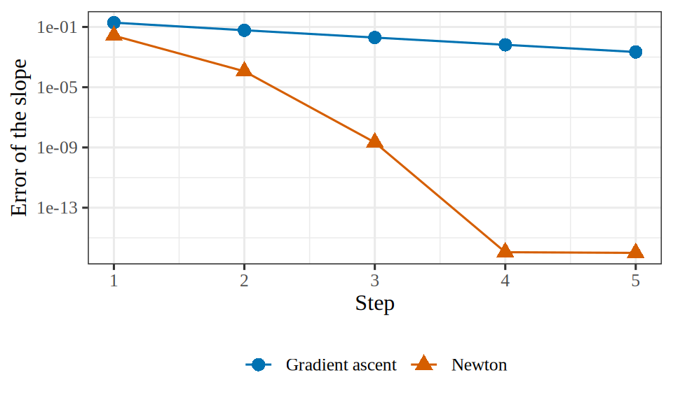
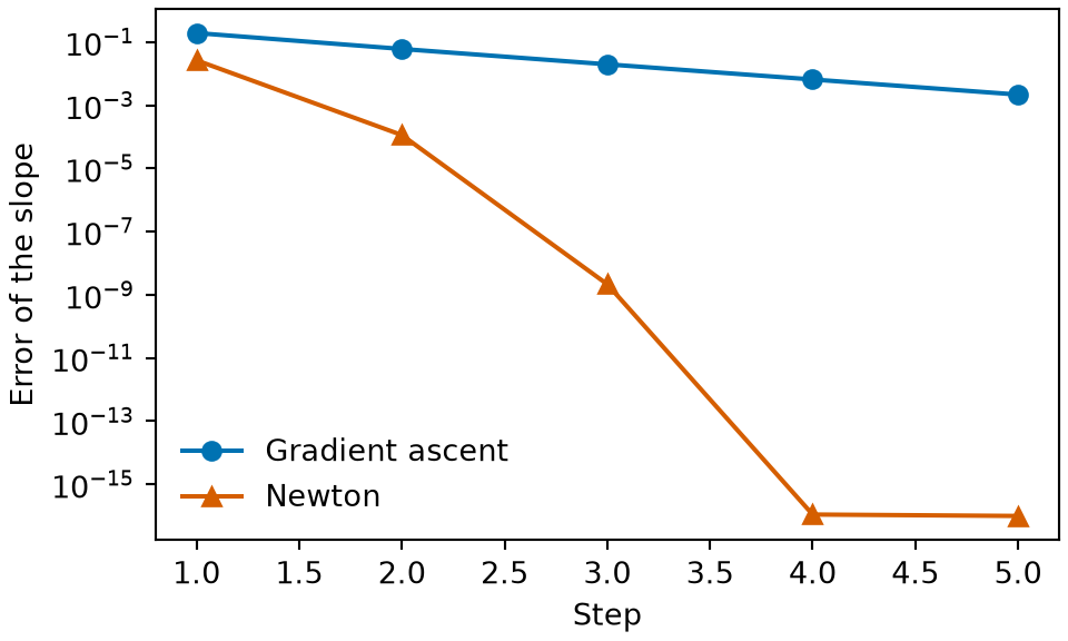
Figure 27: The error of the slope coefficient at each step of gradient ascent and of Newton’s method, with errors below \(10^{-16}\) drawn at \(10^{-16}\).
(a)
Line plot of the error of the slope coefficient on a logarithmic vertical axis, against the step, from 1 to 5. The gradient ascent curve, with circles, falls by a factor of about 3 per step, from about 0.19 at step 1 to about 0.002 at step 5. The Newton curve, with triangles, falls much faster, from about 0.03 at step 1 to about 1e-4 at step 2, 2e-9 at step 3, and the level of rounding error, 1e-16, at steps 4 and 5.
(b)
Line plot of the error of the slope coefficient on a logarithmic vertical axis, against the step, from 1 to 5. The gradient ascent curve, with circles, falls by a factor of about 3 per step, from about 0.19 at step 1 to about 0.002 at step 5. The Newton curve, with triangles, falls much faster, from about 0.03 at step 1 to about 1e-4 at step 2, 2e-9 at step 3, and the level of rounding error, 1e-16, at steps 4 and 5.

Exercise 94 (Newton’s method: the cost of one step)

Exercise 94 (Newton’s method: the cost of one step) Use the setup of Exercise 93.

How many arithmetic operations does one step of gradient ascent take, and how many does one step of Newton’s method take, for \(\nobs\) observations and a design matrix with \(\ninputvars + 1\) columns?

Solution 94. A gradient step computes \(\design \vcoef\) and \(\tp{\design} \paren{\voutvar - \vprob}\), each \(O(\nobs\ninputvars)\). A Newton step also forms \(\tp{\design} W \design\), which is \(O(\nobs\ninputvars^2)\), and solves a \((\ninputvars + 1) \times (\ninputvars + 1)\) system of equations, which is \(O(\ninputvars^3)\).

Exercise 95 (Newton’s method, and why it is a weighted least squares fit (part 10))

Exercise 95 (Newton’s method, and why it is a weighted least squares fit (part 10)) Use the setup of Exercise 80.

Using the operation counts of Exercise 94, state when Newton’s method needs less computation overall than gradient ascent.

Solution 95. Dividing the operation count of a Newton step by that of a gradient step gives

\[ \frac{\nobs\ninputvars^2 + \ninputvars^3}{\nobs\ninputvars} = \ninputvars + \frac{\ninputvars^2}{\nobs}, \]

which is at most \(2\ninputvars\) when \(\nobs \ge \ninputvars\). So one Newton step costs on the order of \(\ninputvars\) gradient steps, and Newton’s method needs less computation overall when it saves more steps than that. Gradient ascent can need many more steps: the simulated fit of Solution 43 ran \(10{,}000\). Newton’s method needs a handful (Exercise 88), so for \(\ninputvars\) up to the hundreds Newton’s method is usually cheaper, which is one reason R’s glm() fits by IRLS [12, Ch. 3].

Exercise 96 (Newton’s method, and why it is a weighted least squares fit (part 11))

Exercise 96 (Newton’s method, and why it is a weighted least squares fit (part 11)) Use the setup of Exercise 80.

Neural networks are usually fitted by first-order methods, such as gradient descent, rather than by Newton’s method. Explain why.

Solution 96. Newton’s method needs the Hessian, a matrix with one row and one column for each parameter. A neural network can have millions of parameters, so its Hessian has \(10^{12}\) or more entries, which at 8 bytes each is 8 terabytes or more: too large to store, and far too large to factorize at \(O(\text{parameters}^3)\) operations per step. The chapter on neural networks therefore fits them by first-order methods, which brings back the choice of learning rate that Newton’s method does not need.

Exercise 97 (Newton’s method, and why it is a weighted least squares fit (part 12))

Exercise 97 (Newton’s method, and why it is a weighted least squares fit (part 12)) Use the setup of Exercise 80.

\(\iterpoint{W}{\iter}\) depends on \(\iterpoint{\vcoef}{\iter}\) and \(\design\) but not on \(\voutvar\). What follows about the observed information and the expected (Fisher) information?

Solution 97. The weight matrix \(W\) is computed from the fitted probabilities, which depend on \(\vcoef\) and \(\design\) alone, so no outcome \(\outvar_i\) appears in the Hessian \(-\tp{\design} W \design\). The Hessian is therefore not random: its expectation over \(\vY\) is the Hessian itself. The observed information \(\oinfm = \tp{\design} W \design\) and the expected information \(\einfm = \E{\tp{\design} W \design}\) are the same matrix, at every \(\vcoef\) and for every dataset.

Exercise 98 (Newton’s method and Fisher scoring)

Exercise 98 (Newton’s method and Fisher scoring) Use the setup of Exercise 97.

What follows for Newton’s method and Fisher scoring on logistic regression?

Solution 98. Newton’s method steps with the observed information, and Fisher scoring steps with the expected information, so for logistic regression the two algorithms take the same steps. The equality comes from the logit link, which is the canonical link of the Bernoulli family [13], not from binary regression in general. Fitting the same data with a probit link, \(\prob_i = \normcdf(\dprod{\vx_i}{\vcoef})\), gives a Hessian that involves the \(\outvar_i\), so there the two information matrices differ and the two algorithms take different steps.

Remark 6 (Fisher information is the curvature of the Kullback–Leibler divergence)

Remark 6 (Fisher information is the curvature of the Kullback–Leibler divergence). The expected (Fisher) information at the true parameter \(\vcoef_0\) equals the Hessian, with respect to \(\vcoef\) and at the true parameter, of the Kullback–Leibler divergence from the true distribution of \(\vY\) to the model’s distribution with parameter \(\vcoef\) (proved in the statistics notes):

\[ \evalAt{\gradwrt{\vcoef}{\tp{\gradwrt{\vcoef}{\kldivf{\p_{\vcoef_0}}{\p_{\vcoef}}}}}}{\vcoef = \vcoef_0} = \einff{\vcoef_0}. \]

The expected cross-entropy loss equals that divergence plus the entropy of the true distribution:

\[ \E{\lossf{\vcoef}} = \kldivf{\p_{\vcoef_0}}{\p_{\vcoef}} + \entropyf{\p_{\vcoef_0}}. \]

The entropy does not depend on \(\vcoef\), so the expected cross-entropy loss and the divergence have the same Hessian at every \(\vcoef\):

\[ \gradwrt{\vcoef}{\tp{\gradwrt{\vcoef}{\E{\lossf{\vcoef}}}}} = \gradwrt{\vcoef}{\tp{\gradwrt{\vcoef}{\kldivf{\p_{\vcoef_0}}{\p_{\vcoef}}}}}. \]

For logistic regression, the Hessian of the cross-entropy loss does not involve the outcomes (Solution 97), so at every \(\vcoef\), not only at the true parameter, it equals the Hessian of the expected cross-entropy loss. That Hessian is the Fisher information:

\[ \gradwrt{\vcoef}{\tp{\gradwrt{\vcoef}{\lossf{\vcoef}}}} = \gradwrt{\vcoef}{\tp{\gradwrt{\vcoef}{\E{\lossf{\vcoef}}}}} = \einff{\vcoef} = \tp{\design} W \design. \]

Fisher scoring therefore scales each step by the curvature of the expected cross-entropy loss at the current iterate, whose sample version logistic regression minimizes:

\[ \iterpoint{\vcoef}{\iter+1} = \iterpoint{\vcoef}{\iter} - \inv{\einff{\iterpoint{\vcoef}{\iter}}} \gradwrt{\vcoef}{\lossf{\iterpoint{\vcoef}{\iter}}}. \]

Watch

Read

GeeksforGeeks explains Newton’s method [15].

[1]
Wikipedia contributors, “Cross-entropy — Wikipedia, the free encyclopedia.” 2026. Available: https://en.wikipedia.org/wiki/Cross-entropy
[2]
V. Guruswami and P. Raghavendra, “Hardness of learning halfspaces with noise,” SIAM Journal on Computing, vol. 39, no. 2, pp. 742–765, 2009, doi: 10.1137/070685798.
[3]
GeeksforGeeks, “What is cross-entropy loss function?” GeeksforGeeks, tutorial article, 2025. Available: https://www.geeksforgeeks.org/machine-learning/what-is-cross-entropy-loss-function/
[4]
C. E. Shannon, “A mathematical theory of communication,” Bell System Technical Journal, vol. 27, no. 3, pp. 379–423, 1948, doi: 10.1002/j.1538-7305.1948.tb01338.x.
[5]
K. Weinberger, “CS4780: Machine learning for intelligent systems, spring 2017.” Cornell University, lecture videos on YouTube, 2017. Available: https://www.youtube.com/playlist?list=PLl8OlHZGYOQ7bkVbuRthEsaLr7bONzbXS
[6]
J. Starmer, “Logistic regression details, part 2: Maximum likelihood.” StatQuest, video on YouTube, 2018. Available: https://www.youtube.com/watch?v=BfKanl1aSG0
[7]
D. M. Rocke, “EPI 204 lecture notes, Spring 2021.” University of California, Davis, 2021. Available: https://dmrocke.ucdavis.edu/Class/EPI204-Spring-2021/EPI204-Spring-2021.html
[8]
J. Starmer, “Neural networks part 6: Cross entropy.” StatQuest, video on YouTube, 2021. Available: https://www.youtube.com/watch?v=6ArSys5qHAU
[9]
GeeksforGeeks, “Binary cross entropy/log loss for binary classification.” GeeksforGeeks, tutorial article, 2025. Available: https://www.geeksforgeeks.org/deep-learning/binary-cross-entropy-log-loss-for-binary-classification/
[10]
F. Pedregosa et al., “Scikit-learn: Machine learning in Python,” Journal of Machine Learning Research, vol. 12, pp. 2825–2830, 2011, Available: https://jmlr.org/papers/v12/pedregosa11a.html
[11]
S. Boyd and L. Vandenberghe, Convex optimization. Cambridge University Press, 2004. doi: 10.1017/CBO9780511804441.
[12]
S. N. Wood, Generalized additive models: An introduction with R, 2nd ed. Chapman; Hall/CRC, 2017. doi: 10.1201/9781315370279.
[13]
J. A. Nelder and R. W. M. Wedderburn, “Generalized linear models,” Journal of the Royal Statistical Society: Series A (General), vol. 135, no. 3, pp. 370–384, 1972, doi: 10.2307/2344614.
[14]
A. Ng et al., “CS229: Machine learning, autumn 2018.” Stanford Online, lecture videos on YouTube, 2018. Available: https://www.youtube.com/playlist?list=PLoROMvodv4rMiGQp3WXShtMGgzqpfVfbU
[15]
GeeksforGeeks, “Newton’s method in machine learning.” GeeksforGeeks, tutorial article, 2025. Available: https://www.geeksforgeeks.org/machine-learning/newtons-method-in-machine-learning/