Generalization and Cross-Validation
Risk, held-out estimates, and cross-validation
Last modified: 2026-11-19
Show code
biCrime = (await FileAttachment("data/crime.csv").csv({typed: true})).map((d) => [d.x, d.y])
// The simulated world of the bias-variance explorer, which needs a known true mean function:
// this function, plus Gaussian noise with standard deviation biSigma, on inputs in [0.05, 0.95].
biTruth = (x) => 0.55 - 0.9 * x + 0.6 * Math.sin(6 * x)
biSigma = 0.1
biXlo = 0.05
biXhi = 0.95
// The real data of the train, cross-validation and nearest-neighbour figures:
// the 392 cars of the Auto data, as (horsepower, mpg) pairs.
// Horsepower is rescaled to [0, 1], which the polynomial basis below assumes,
// and mpg is standardized to mean 0 and standard deviation 1,
// so that a squared error is a fraction of the variance of mpg.
// biHpAxis, biMpgAxis and biMpgUnits below turn both back into horsepower and mpg
// wherever a figure labels an axis or a number.
biAuto = FileAttachment("data/auto.csv").csv({typed: true})
biHpRange = d3.extent(biAuto, (d) => d.horsepower)
biMpgMean = d3.mean(biAuto, (d) => d.mpg)
biMpgSd = d3.deviation(biAuto, (d) => d.mpg)
biCars = biAuto.map((d) => [
  (d.horsepower - biHpRange[0]) / (biHpRange[1] - biHpRange[0]),
  (d.mpg - biMpgMean) / biMpgSd
])
// Axes in the original units, drawn on the scaled data.
// Every axis shows ticks in the units the variable was measured in,
// however the model is parametrized: the scaled value x sits at the tick
// labelled with its horsepower, and the standardized value y at its mpg.
biHpAxis = ({
  label: "horsepower",
  ticks: d3.range(50, biHpRange[1] + 1e-9, 50)
    .map((hp) => (hp - biHpRange[0]) / (biHpRange[1] - biHpRange[0])),
  tickFormat: (x) => Math.round(biHpRange[0] + x * (biHpRange[1] - biHpRange[0]))
})
biMpgAxis = ({
  label: "mpg",
  ticks: d3.range(10, 51, 10).map((mpg) => (mpg - biMpgMean) / biMpgSd),
  tickFormat: (y) => Math.round(biMpgMean + y * biMpgSd)
})
// An RMSE in standardized units, converted to miles per gallon.
biMpgUnits = (v) => v * biMpgSd
// An interval printed as [lo, hi] in miles per gallon, to two decimals.
biFmtCIMpg = (ci) => `[${biMpgUnits(ci.lo).toFixed(2)}, ${biMpgUnits(ci.hi).toFixed(2)}]`
// n cars chosen at random as a training set, reproducibly from an integer seed;
// the held-out set is every car not chosen.
biCarSplit = (n, seed) => {
  const order = d3.shuffler(d3.randomLcg(seed))(d3.range(biCars.length));
  return {
    train: order.slice(0, n).map((i) => biCars[i]),
    held: order.slice(n).map((i) => biCars[i])
  };
}
// An evenly spaced grid of horsepower values, for drawing curves over the cars.
biCarGrid = d3.range(0, 1 + 1e-9, 1 / 200)
// Least-squares polynomial of the given degree, returned as a function of x.
// The basis is Chebyshev polynomials of t = 2x - 1, and the system is solved by
// Householder QR, so degrees up to about 10 stay well conditioned on [0, 1].
biBasis = (x, degree) => {
  const t = 2 * x - 1;
  const row = [1, t];
  for (let j = 2; j <= degree; j++) row.push(2 * t * row[j - 1] - row[j - 2]);
  return row.slice(0, degree + 1);
}
// A degree of n - 1 or more interpolates n points, so it is capped there.
biPolyfit = (pts, deg) => {
  const n = pts.length;
  const degree = Math.min(deg, n - 1);
  const p = degree + 1;
  const a = pts.map(([x]) => biBasis(x, degree));
  const b = pts.map(([, y]) => y);
  for (let k = 0; k < p; k++) {
    let norm = 0;
    for (let i = k; i < n; i++) norm += a[i][k] ** 2;
    norm = Math.sqrt(norm);
    if (norm === 0) continue;
    const alpha = a[k][k] > 0 ? -norm : norm;
    const v = [];
    for (let i = k; i < n; i++) v.push(a[i][k]);
    v[0] -= alpha;
    const vv = v.reduce((s, e) => s + e * e, 0);
    if (vv === 0) continue;
    for (let j = k; j < p; j++) {
      let s = 0;
      for (let i = k; i < n; i++) s += v[i - k] * a[i][j];
      for (let i = k; i < n; i++) a[i][j] -= 2 * v[i - k] * s / vv;
    }
    let s = 0;
    for (let i = k; i < n; i++) s += v[i - k] * b[i];
    for (let i = k; i < n; i++) b[i] -= 2 * v[i - k] * s / vv;
  }
  const c = new Array(p).fill(0);
  for (let k = p - 1; k >= 0; k--) {
    let s = b[k];
    for (let j = k + 1; j < p; j++) s -= a[k][j] * c[j];
    c[k] = a[k][k] === 0 ? 0 : s / a[k][k];
  }
  return (x) => biBasis(x, degree).reduce((s, e, j) => s + e * c[j], 0);
}
// Mean squared error of a prediction function h on a set of points.
biMse = (h, pts) => d3.mean(pts, ([x, y]) => (h(x) - y) ** 2)
// A 95% confidence interval for the risk of h (its mean squared error over the population),
// from the squared errors of h on points it was not fitted to.
// By the central limit theorem the mean of n squared errors is close to normal,
// with standard error sd / sqrt(n), so the interval is the mean plus or minus 1.96 standard errors.
// The held-out sets here have at least 190 cars, so 1.96 stands in for the t quantile.
// It is not meant for points the model was fitted to, whose errors are not independent draws.
biMseCI = (h, pts) => {
  const errs = pts.map(([x, y]) => (h(x) - y) ** 2);
  const m = d3.mean(errs);
  const half = 1.96 * d3.deviation(errs) / Math.sqrt(errs.length);
  return {mean: m, lo: m - half, hi: m + half};
}
// The root mean squared error (RMSE) of h on a set of points, in the units of the response,
// and the same interval as biMseCI with its endpoints square-rooted.
biRmse = (h, pts) => Math.sqrt(biMse(h, pts))
biRmseCI = (h, pts) => {
  const ci = biMseCI(h, pts);
  return {mean: Math.sqrt(ci.mean), lo: Math.sqrt(Math.max(ci.lo, 0)), hi: Math.sqrt(ci.hi)};
}
// The RMSE interval for a short list of squared errors, one per case, by the percentile bootstrap:
// resample the errors with replacement 1,000 times, take the root of each resample's mean,
// and keep the 2.5th and 97.5th percentiles of those roots.
// Cross-validation uses it on the held-out squared errors, one per point.
// With so few skewed errors, the interval 1.96 standard errors either side of the mean
// can reach below zero, which a root mean squared error cannot do; the bootstrap never does.
// The seed fixes the resamples, so the interval does not change when the page redraws.
biRmseCIBoot = (sq, seed = 1) => {
  const rand = d3.randomLcg(seed);
  const n = sq.length;
  const roots = d3.range(1000).map(() =>
    Math.sqrt(d3.mean(d3.range(n), () => sq[Math.floor(rand() * n)])));
  roots.sort(d3.ascending);
  return {mean: Math.sqrt(d3.mean(sq)), lo: d3.quantileSorted(roots, 0.025),
          hi: d3.quantileSorted(roots, 0.975)};
}
// Print an interval as [lo, hi] to four decimals.
biFmtCI = (ci) => `[${ci.lo.toFixed(4)}, ${ci.hi.toFixed(4)}]`
// Tick marks for a log axis: the powers of ten from lo to hi, printed in plain
// decimals (0.001, 1,000), never in scientific notation.
// Plot's default log ticks label every minor tick, which crowds a short axis.
biPow10 = (lo, hi) => d3.range(Math.round(Math.log10(lo)), Math.round(Math.log10(hi)) + 1)
  .map((e) => 10 ** e)
biExp = (v) => d3.format(",.8~f")(v)
Source
Adapted from Brian Hutchinson’s Fall 2025 lecture notes, which supplied the crime-and-income example and the generalization argument. Logan Sizemore’s Spring 2025 lecture on generalization is the basis of the cross-validation section. The wider reading is Hastie et al. [1], Chapter 2, and James et al. [2], Chapter 2.
1 Generalization
Watch
Hutchinson covers generalization, bias, variance and overfitting, in the video Generalization (31 min) [3].
Definition 1 (Objective function (objective))
Definition 1 (Objective function (objective)) An objective function, or objective for short [4, Sec. 1.1] and 4.1, is the quantity training optimizes as the model’s parameters vary, by minimizing it or by maximizing it. It is a function of the parameters alone, with the data held fixed. For a model \(\modmemof{\param}\) with parameters \(\param\) and a training set \(\trainset\), the objective that is the empirical risk is
\[ \objfnf{\param} \eqdef \empriskf{\modmemof{\param}; \trainset} , \tag{1}\]
and training minimizes \(\objfnf{\param}\) over \(\param\).
Example 1 (The objective as a function of the slope and intercept)
Example 1 (The objective as a function of the slope and intercept) For the crime data, the objective is the empirical risk as a function of the pair \((m, b)\).
[1] 0.023056 0.002721The flat line \((m, b) = (0, \bar y)\) has objective value \(0.023056\), and the least-squares pair \((\hat m, \hat b) = (-1.2877, 0.7052)\) has the smaller value \(0.002721\). Training searches over \((m, b)\) for the pair with the smallest value.
Remark 1 (The empirical risk is one objective among many)
Remark 1 (The empirical risk is one objective among many). So far the only objective in these notes is the empirical risk, which the minimization problem minimizes over the slope and intercept. Later chapters change the objective without changing the loss: whatever is handed to the optimizer is the objective, and the empirical risk is only one thing it can be made from.
Definition 2 (Cost function)
Definition 2 (Cost function) A cost function is an objective function for which smaller values are better.
Example 2 (The empirical risk of the crime data as a cost function)
Example 2 (The empirical risk of the crime data as a cost function) For the crime data, the objective of Example 1 is the empirical risk under squared-error loss, which is a cost function: \[ \objfnf{m, b} = \frac{1}{n} \sum_{i=1}^n (m x_i + b - y_i)^2 . \] A line farther from the data has a larger value.
[1] 0.002721 0.119961The pair \((\hat m, \hat b)\) from lm has cost \(0.002721\), and raising the slope by 1 raises the cost to \(0.119961\). Training moves toward smaller values, so it minimizes this cost. Figure 1 plots both against the data.
Show code
crime_points <- tibble::tibble(x = x, y = y)
crime_points |>
  ggplot2::ggplot() +
  ggplot2::aes(x = x, y = y) +
  ggplot2::geom_point() +
  ggplot2::geom_abline(intercept = b_hat, slope = m_hat, colour = "#0072B2") +
  ggplot2::geom_abline(
    intercept = b_hat,
    slope = m_hat + 1,
    colour = "#D55E00"
  ) +
  ggplot2::expand_limits(y = 0.7) +
  ggplot2::labs(x = "Per-capita income", y = "Crime rate")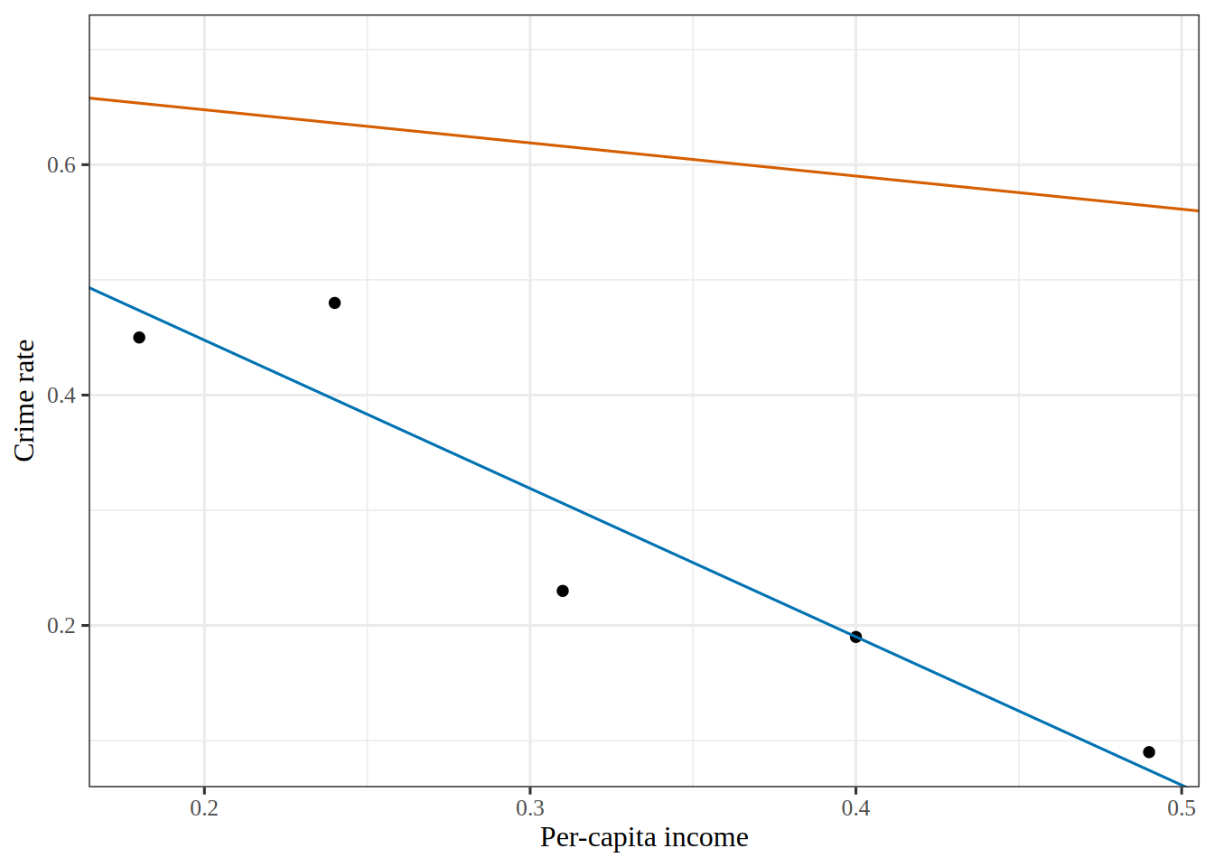
Remark 2 (How the loss, the empirical risk, the objective function and the cost function relate)
Remark 2 (How the loss, the empirical risk, the objective function and the cost function relate). Four related quantities answer different questions.
- The loss function assesses one prediction.
- The empirical risk is the loss averaged over the \(n\) examples in the training set, so it assesses a model on the whole training set.
- The objective function is whatever training optimizes as the parameters vary. So far it is the empirical risk. For a penalized fit such as the one in the ridge regression section, it combines the empirical risk, or a multiple of it, with a penalty.
- A cost function is an objective function for which smaller values are better, so training minimizes it. The log-likelihood is an objective function that training maximizes, so minus the log-likelihood is a cost function. Other texts also use “cost function” for the loss function or for the empirical risk, but here it always refers to a minimized objective function.
Under squared-error loss, the empirical risk is the sample mean squared error, and the residual sum of squares is \(n\) times that empirical risk. The two differ only by the factor \(n \ge 1\), so they have the same minimizers.
Exercise 1 (Estimate what cannot be computed)
Exercise 1 (Estimate what cannot be computed) The risk cannot be evaluated, and the empirical risk can. The solution to “Which model was actually better?” rules out reporting the second in place of the first.
Describe a procedure that uses only the available data and returns an honest estimate of the risk, and say what the procedure costs.
Solution 1. Set some data aside. Split \(\trainset\) before fitting anything; fit on one part; score on the other. The scored part played no role in choosing the model’s parameters, so the sample mean of its losses is an unbiased estimate of the risk: over repeated draws of the held-out points, it equals the risk on average, neither systematically above nor below.
The cost is the data itself. Points moved into the held-out set are points the model never learns from, so the model is worse than it needed to be, and the estimate depends on however few points were set aside and is noisy in proportion.
The usual arrangement is three sets rather than two:
A training set, which the fit uses.
A validation set (Definition 3; also called a development or dev set), scored repeatedly while choosing between models, tuning their settings, and deciding when to stop.
A test set (Definition 5), scored exactly once, at the end, on the model finally chosen. It stays unused until then.
The third set exists because of what the second one does. A validation set consulted a hundred times is a set a hundred decisions have been fitted to, and its score stops being honest about a model those decisions selected. Section 1.1 covers what to do when there is not enough data for all three.
Example 3 (Splitting the Auto data)
Example 3 (Splitting the Auto data) Split the cars of the Auto data [2] at random, 60% for training, 20% for validation and the rest for testing.
# Draw the three index sets from one shuffled list of cars, so that they cannot overlap.
import numpy as np
import pandas as pd

auto_split = pd.read_csv("data/auto.csv").dropna(subset=["horsepower"])
n_cars = len(auto_split)
shuffled = np.random.default_rng(571).permutation(n_cars)
n_train = int(0.6 * n_cars)
n_val = int(0.2 * n_cars)
idx_train = shuffled[:n_train]
idx_val = shuffled[n_train:n_train + n_val]
idx_test = shuffled[n_train + n_val:]
print(n_train, n_val, len(idx_test))
235 78 79Of the 392 cars with a recorded horsepower, 235 form the training set, which is all the fitting procedure sees, and the other 157 are held out of the fit.
Definition 3 (Validation set)
Definition 3 (Validation set) A validation set is a subset of the data set, the pairs indexed by a set \(\validx\) that shares no index with \(\trainidx\), and that we use for model selection among candidate models fitted to the training set [5]:
\[ \valset \eqdef \set{(\vpredvar_i, \outvar_i) : i \in \validx} \subseteq \dataset, \quad \validx \cap \trainidx = \emptyset . \tag{2}\]
The model with the smallest empirical risk on the validation set is the one we keep.
Definition 4 (Validation error)
Definition 4 (Validation error) The validation error of a model \(\modmem\) is its empirical risk on the validation set, \(\empriskf{\modmem; \valset}\).
See validation error in the statistics notes.
Example 4 (Choosing a polynomial degree)
Example 4 (Choosing a polynomial degree) Fit polynomials of degree 1 to 9 to the 235 training cars of Example 3, predicting mpg from horsepower, and score each on the 78 validation cars.
# Scale horsepower to 0 to 1 so that high degrees are numerically stable.
hp = auto_split["horsepower"].to_numpy(dtype=float)
hp = (hp - hp.min()) / (hp.max() - hp.min())
mpg = auto_split["mpg"].to_numpy(dtype=float)

def mse(coef, idx):
    return np.mean((np.polyval(coef, hp[idx]) - mpg[idx]) ** 2)

degrees = range(1, 10)
fits = {d: np.polyfit(hp[idx_train], mpg[idx_train], d) for d in degrees}
val_mse = {d: mse(fits[d], idx_val) for d in degrees}
train_mse = {d: mse(fits[d], idx_train) for d in degrees}
best_degree = min(val_mse, key=val_mse.get)
train_mse_9 = train_mse[9]
val_mse_9 = val_mse[9]
val_mse_best = val_mse[best_degree]

def mse_ci(coef, idx):
    # Normal-approximation 95% interval for the mean of the squared errors.
    sq = (np.polyval(coef, hp[idx]) - mpg[idx]) ** 2
    se = sq.std(ddof=1) / np.sqrt(len(sq))
    return sq.mean() - 1.96 * se, sq.mean() + 1.96 * se

val_ci_best = mse_ci(fits[best_degree], idx_val)
val_ci_9 = mse_ci(fits[9], idx_val)
print(best_degree, round(val_mse[best_degree], 3), round(train_mse_9, 3), round(val_mse_9, 3))
2 18.006 16.78 19.559[12.012 23.999] [11.9 27.218]The degree with the smallest validation error, 2, is the one we keep. The training cars could not make this choice, because the training error keeps falling as the degree grows: the degree-9 fit has training error 16.78 and validation error 19.56. The chosen degree’s validation error, 18.01, has a 95% confidence interval of 12.01 to 24.00, and the degree-9 fit’s has 11.90 to 27.22. Each interval comes from the 78 validation cars alone, and the chosen degree’s is optimistic, because the same cars picked the degree.
Definition 5 (Test set)
Definition 5 (Test set) A test set is a subset of the data set, the pairs indexed by a set \(\testidx\) that shares no index with \(\trainidx\) or \(\validx\), and that we use only once, after the model is chosen, to estimate the risk of the chosen model \(\modmem\) by its empirical risk on the test set, \(\empriskf{\modmem; \testset}\):
\[ \testset \eqdef \set{(\vpredvar_i, \outvar_i) : i \in \testidx} \subseteq \dataset, \quad \testidx \cap \paren{\trainidx \cup \validx} = \emptyset . \tag{3}\]
Definition 6 (Test error)
Definition 6 (Test error) The test error of a model \(\modmem\) is its empirical risk on the test set, \(\empriskf{\modmem; \testset}\).
See test error in the statistics notes.
Example 5 (Reporting the chosen degree’s error)
Example 5 (Reporting the chosen degree’s error) Having chosen degree 2 on the validation cars of Example 4, score that one model on the 79 test cars.
# Refit the chosen degree on the training cars of @exm-training-set (scaled horsepower hp, mpg),
# so this chunk does not lean on the fits table of the validation example.
chosen_coef = np.polyfit(hp[idx_train], mpg[idx_train], best_degree)
# A normal-approximation 95% interval: the mean of the squared errors
# plus or minus 1.96 standard errors.
test_sq = (np.polyval(chosen_coef, hp[idx_test]) - mpg[idx_test]) ** 2
test_mse = np.mean(test_sq)
test_se = test_sq.std(ddof=1) / np.sqrt(len(test_sq))
test_lo, test_hi = test_mse - 1.96 * test_se, test_mse + 1.96 * test_se
print(round(test_mse, 3), round(test_lo, 3), round(test_hi, 3))
24.232 14.183 34.281The estimate of the chosen model’s risk is 24.23, with a 95% confidence interval of 14.18 to 34.28. The test cars played no part in the fit or the choice, so the choice did not tune this estimate to them. If it disappoints and we go back to choose again, the test cars have become a validation set.
Definition 7 (Generalization gap)
Definition 7 (Generalization gap) The generalization gap of a model \(\modmem\) on a training set \(\trainset\) is its risk minus its training error [6, Sec. 5.2]:
\[ \popriskf{\modmem} - \empriskf{\modmem; \trainset} . \tag{4}\]
Example 6 (Estimating the chosen degree’s gap)
Example 6 (Estimating the chosen degree’s gap) The risk in Equation 4 cannot be computed, so estimate it by the test error of Example 5, and subtract the training error of the same degree-2 fit.
17.693 24.232 6.539The training error is 17.69 and the test error is 24.23, so the estimated gap is 6.54. The estimate is noisy: the 95% interval for the test error in Example 5 runs from 14.18 to 34.28, and it contains the training error, so these cars alone do not show that the gap is positive.
Remark 3 (The three sets together)
Remark 3 (The three sets together). The three index sets \(\trainidx\), \(\validx\) and \(\testidx\) are disjoint and together cover \(1, \ldots, n\), so the training, validation and test sets are disjoint subsets that together make up the data set \(\dataset\), which is why Example 3 draws them from one shuffled list. The sets are not interchangeable: the first is for fitting, the second for choosing among fits, and the third for reporting. Data used for one job gives an optimistic answer to the next, as Figure 2 shows. Any pairs kept out of the fit are called held-out, so validation and test sets are both held-out sets.
The statistics notes define the same three sets formally: the training set, the validation set, and the test set. They use a different symbol for the training set and a plain observation index, but the same three-way split.
Remark 4 (What the validation and test errors estimate)
Remark 4 (What the validation and test errors estimate). Like the training error, the validation error and the test error are empirical risks, and they differ only in the set that scores the model. The model was not fitted to the validation or test set, so each estimates the risk \(\popriskf{\modmem}\) without the optimism of the training error. We choose the model with the smallest validation error, so the validation error of the chosen model is still optimistic. We compute the test error once, after the choice, so it is not.
Some textbooks use “test error” for the expected error of the fitted model on a new observation, which is the risk of the fitted model, not a number computed from a test set [1, Sec. 7.2]. Here the test error is the number computed from the test set, and the risk is what it estimates.
These ideas hold for any loss, not only squared error. Each error is the average loss on the set that scores the model: the training error, the validation error and the test error. The expected loss of the fitted model on a new observation is its generalization error, the risk of the fitted model. Averaging the generalization error over training sets gives the expected generalization error.
Show code
tvSplit = biCarSplit(tvN, 2100 + tvDraw)
tvTrain = tvSplit.train
tvHeld = tvSplit.held
tvDegrees = d3.range(0, 10)
// Every degree's fit to the training sample, scored on both samples.
tvScores = tvDegrees.map((degree) => {
  const h = biPolyfit(tvTrain, degree);
  return {degree, h, train: biRmse(h, tvTrain), held: biRmse(h, tvHeld), heldCI: biRmseCI(h, tvHeld)};
})
tvFit = tvScores[tvDegree]
tvLong = tvScores.flatMap((d) => [
  {degree: d.degree, set: "training points", rmse: biMpgUnits(d.train)},
  {degree: d.degree, set: "held-out points", rmse: biMpgUnits(d.held),
   lo: Math.max(biMpgUnits(d.heldCI.lo), 1e-1), hi: biMpgUnits(d.heldCI.hi)}
])
In Figure 2, change the degree and the number of training points, and compare the two error curves.
Show code
Show code
md`Degree ${tvDegree}, fitted to ${tvN} training points.
Root mean squared error (RMSE) on the training points: **${biMpgUnits(tvFit.train).toFixed(2)} mpg**;
on the ${tvHeld.length} held-out cars: **${biMpgUnits(tvFit.held).toFixed(2)} mpg**,
with a 95% confidence interval of **${biFmtCIMpg(tvFit.heldCI)}** mpg.`
Show code
Plot.plot({
  ariaLabel: 'The held-out cars as light grey dots, the training cars as black dots, ' +
    'and the least-squares polynomial of the chosen degree as a solid blue curve, ' +
    'with horsepower on the horizontal axis and mpg on the vertical axis.',
  width: 300, height: 260, grid: true,
  x: {domain: [0, 1], ...biHpAxis},
  y: {domain: [-2, 3.5], ...biMpgAxis},
  marks: [
    Plot.dot(tvHeld, {x: (d) => d[0], y: (d) => d[1], r: 2, fill: "#bbb"}),
    Plot.line(biCarGrid, {x: (x) => x, y: tvFit.h, stroke: "#1f77b4", strokeWidth: 2.5, clip: true}),
    Plot.dot(tvTrain, {x: (d) => d[0], y: (d) => d[1], r: 4, fill: "#222"})
  ]
})
Show code
Plot.plot({
  ariaLabel: 'Root mean squared error in miles per gallon, on a log scale, against polynomial degree from 0 to 9, ' +
    'one curve for the training points and one for the held-out points, ' +
    'with a 95% confidence interval drawn around each held-out point, ' +
    'and the chosen degree marked by a vertical line.',
  width: 300, height: 260, marginLeft: 50, grid: true,
  x: {domain: [0, 9], label: "degree", ticks: tvDegrees},
  y: {type: "log", domain: [1e-1, 1e2], clamp: true, label: "RMSE (mpg, log scale)",
      ticks: biPow10(1e-1, 1e2), tickFormat: biExp},
  color: {domain: ["training points", "held-out points"], range: ["#1f77b4", "#ff7f0e"],
          legend: true},
  marks: [
    Plot.ruleX([tvDegree], {stroke: "#888"}),
    // The 95% confidence interval of each held-out error, as a vertical bar.
    Plot.ruleX(tvLong.filter((d) => d.set === "held-out points"),
      {x: "degree", y1: "lo", y2: "hi", stroke: "set", strokeWidth: 1.5}),
    Plot.line(tvLong, {x: "degree", y: "rmse", stroke: "set", strokeWidth: 2}),
    Plot.dot(tvLong, {x: "degree", y: "rmse", fill: "set", r: 3})
  ]
})Remark 5 (Reading the figure on training and held-out error)
Remark 5 (Reading the figure on training and held-out error). The polynomials are fitted with horsepower scaled to run from 0 to 1 and mpg standardized, but every axis and number here is in the original units, horsepower and miles per gallon. The sRMSE is the square root of the sample mean squared error, so it is in the units of the response, here miles per gallon (why we report sRMSE). The vertical bars on the held-out curve and the interval in the readout are 95% confidence intervals for the held-out sRMSE: the mean of the squared errors plus or minus 1.96 standard errors, from the central limit theorem, with the endpoints square-rooted. It is rough when a high-degree fit makes a few squared errors enormous, and it describes the risk of this fitted polynomial, not of the fitting method. The training error has no interval: the fit was chosen to make those errors small, so they are not independent draws and their mean is biased low as an estimate of the risk, and an interval around it would be centered in the wrong place.
Exercise 2 (How far can a held-out score be trusted?)
Exercise 2 (How far can a held-out score be trusted?) A spam filter \(\modmem\) was trained on one set of emails and then scored on a fresh held-out set \(\mathcal{V}\) of \(n\) emails, drawn independently from the same distribution as the emails it will face. Its held-out score \(\empriskf{\modmem; \mathcal{V}}\) is the fraction of those emails it labels wrong, and its risk \(\popriskf{\modmem}\) is its error rate on the population.
Find an upper bound on the chance that the held-out score misses the risk by more than some \(\tolout > 0\), using only the mean and variance of the held-out score.
Solution 2. Write \(Z_i\) for the loss on the \(i\)th held-out email: 1 if \(\modmem\) labels it wrong, and 0 if right. The filter was fixed before \(\mathcal{V}\) was drawn, so the \(Z_i\) are independent, and each is 1 with probability \(\popriskf{\modmem}\). The held-out score is their average, \(\empriskf{\modmem; \mathcal{V}} = \avgin Z_i\), so its mean is \(\popriskf{\modmem}\).
Its variance is the variance of one \(Z_i\) divided by \(n\). A 0/1 variable that is 1 with probability \(R\) has variance \(R(1 - R)\), and that is never more than \(\frac{1}{4}\):
\[ R(1 - R) = \frac{1}{4} - \paren{ R - \frac{1}{2} }^2 \le \frac{1}{4} . \]
So \(\Var{\empriskf{\modmem; \mathcal{V}}} \le \frac{1}{4n}\), whatever the filter’s error rate is. Chebyshev’s inequality bounds the chance of a miss by the variance divided by the square of the miss:
\[ P\paren{ \abs{ \empriskf{\modmem; \mathcal{V}} - \popriskf{\modmem} } > \tolout } \le \frac{\Var{\empriskf{\modmem; \mathcal{V}}}}{\tolout^2} \le \frac{1}{4 n \tolout^2} . \]
Exercise 3 (How far can a held-out score be trusted? (part 2))
Exercise 3 (How far can a held-out score be trusted? (part 2)) Use the setup of Exercise 2.
How does your bound change as \(n\) grows?
Solution 3. The bound shrinks in proportion to \(1/n\): ten times as many held-out emails make a miss of a given size at most a tenth as likely.
For example, with \(n = 1000\) and \(\tolout = 0.05\), the chance of a miss is at most \(1 / (4 n \tolout^2) = 0.1\).
Chebyshev uses only the variance, and the 0/1 range entered only through the cap of \(\frac{1}{4}\) on it. Using the range itself, that each \(Z_i\) lies between 0 and 1, gives a much sharper bound, one that shrinks exponentially in \(n\) rather than in proportion to \(1/n\).
Theorem 1 (Hoeffding’s inequality for a held-out set)
Theorem 1 (Hoeffding’s inequality for a held-out set) Score a classifier \(\modmem\) with the misclassification loss. Let \(\valset\) be a held-out set of \(n\) observations drawn independently from the same distribution \(P(x, y)\), and let \(\empriskf{\modmem; \valset}\) be the fraction of them \(\modmem\) gets wrong, as in the definition of the empirical risk. If \(\modmem\) is fixed before \(\valset\) is drawn, then for every \(\tolout > 0\) [7],
\[ P\paren{ \abs{ \empriskf{\modmem; \valset} - \popriskf{\modmem} } > \tolout } \le 2 e^{-2 \tolout^2 n} . \tag{5}\]
Proof
Proof. The misclassification loss of \(\modmem\) on the \(i\)th held-out point, \(\lossf{y_{(i)}, \modmemf{x_{(i)}}}\), is 1 when \(\modmem\) gets the point wrong and 0 otherwise. Because \(\modmem\) is fixed before \(\valset\) is drawn, each loss is the same function of one of \(n\) independent draws from \(P(x, y)\). So the \(n\) losses are IID random variables in \([0, 1]\). Their common population mean is \(\popriskf{\modmem}\) by the definition of the risk, and their sample mean is \(\empriskf{\modmem; \valset}\) by the definition of the empirical risk. Hoeffding’s inequality for an average of IID variables in \([0, 1]\) bounds the chance that the average misses the mean by at least \(\tolout\) by \(2 e^{-2 \tolout^2 n}\). The event “misses by more than \(\tolout\)” is part of that event, so its chance is at most as large.
Remark 6 (Reading Hoeffding’s inequality)
Remark 6 (Reading Hoeffding’s inequality). The misclassification loss is 1 when \(\modmemf{x} \neq y\) and 0 otherwise, so \(\popriskf{\modmem}\), the risk, is the error rate of the classifier on the population. The probability in Equation 5 is over the draw of \(\mathcal{V}\); \(\popriskf{\modmem}\) is unknown but not random.
Exercise 4 (How many held-out emails are enough?)
Exercise 4 (How many held-out emails are enough?) A spam filter was trained on one set of emails, and you will estimate its error rate on a fresh held-out set. Say the estimate misses when it differs from the filter’s true error rate by more than 0.05.
How many held-out emails make the chance of a miss at most 0.05?
Solution 4. In Exercise 4, the filter was fixed before the held-out set was drawn, so Equation 5 applies. Write \(\tolout\) for the allowed miss and \(\tolin\) for the allowed chance. The chance of a miss is at most \(\tolin\) whenever the bound is:
\[ \begin{aligned} 2 \e{-2 \tolout^2 \nobs} &\le \tolin \\ \e{-2 \tolout^2 \nobs} &\le \frac{\tolin}{2} \\ -2 \tolout^2 \nobs &\le \ln \frac{\tolin}{2} \\ 2 \tolout^2 \nobs &\ge -\ln \frac{\tolin}{2} = \ln \frac{2}{\tolin} \\ \nobs &\ge \frac{\ln (2 / \tolin)}{2 \tolout^2} . \end{aligned} \]
The fourth line multiplies both sides by \(-1\), which flips the inequality, and the fifth divides by \(2 \tolout^2\).
With \(\tolout = 0.05\) and \(\tolin = 0.05\), that is \(\nobs \ge 738\) emails. The bound is loose, so fewer emails may well do, but 738 are enough whatever the classifier’s error rate is.
Exercise 5 (How many held-out emails are enough? (part 2))
Exercise 5 (How many held-out emails are enough? (part 2)) Use the setup of Exercise 4.
Suppose instead that 100 different filters, all trained before the held-out set was drawn, are scored on the same held-out set, and you keep the one with the lowest score. How many held-out emails make the chance that the kept filter’s estimate misses at most 0.05?
Solution 5. In Exercise 5, the kept filter was chosen by its held-out score, so it was not fixed before the held-out set was drawn, and Equation 5 does not apply to it directly.
It does apply to each of the \(M = 100\) filters \(\modmemof{1}, \ldots, \modmemof{M}\), since each was trained before the held-out set was drawn. The kept filter’s estimate can miss only if at least one filter’s estimate does, and the chance that at least one of several events happens is at most the sum of their chances. So
\[ \begin{aligned} P\paren{ \text{the kept filter misses} } &\le P\paren{ \text{some } \modmemof{m} \text{ misses} } \\ &\le \sumto{m}{M} P\paren{ \abs{ \empriskf{\modmemof{m}; \mathcal{V}} - \popriskf{\modmemof{m}} } > \tolout } \\ &\le \sumto{m}{M} 2 \e{-2 \tolout^2 \nobs} \\ &= 2 M \e{-2 \tolout^2 \nobs} , \end{aligned} \]
where the third line applies Equation 5 to each term.
Repeating the steps of Solution 4 with \(2M\) in place of 2 gives \(\nobs \ge \ln (2M / \tolin) / (2 \tolout^2)\), which is 1659 emails, about 2.2 times as many as for one filter.
Both answers are sufficient sizes, not required ones, since they come from an upper bound. Two things still follow for Solution 1’s three sets. The sufficient \(\nobs\) is proportional to \(1 / \tolout^2\), so halving the allowed miss quadruples it: with \(\tolout = 0.025\), Solution 4 needs 2952 emails rather than 738. And a validation set on which a fixed list of \(M\) models is compared needs the size from Solution 5 for that \(M\), \(\ln (2M / \tolin) / (2 \tolout^2)\), while a test set scored once on one model needs only the size from Solution 4. The union bound covers only a finite list of models; tuning a setting that can take infinitely many values needs the further analysis that Abu-Mostafa et al. [8] defers to its chapter 2.
Show code
# HTML formats get an interactive plotly figure; the handout and other formats
# get the same curves as a static SVG from tools/make_big_ideas_figures.py.
if (knitr::is_html_output()) {
  library(plotly)

  # Hoeffding's bound 2 exp(-2 tol^2 n), capped at 1 because a probability
  # cannot exceed 1.
  n_held_out <- seq(0, 2000, length.out = 401)
  bound <- function(tol) pmin(1, 2 * exp(-2 * tol^2 * n_held_out))

  widget <- plot_ly() |>
    add_trace(
      x = n_held_out, y = bound(0.1), type = "scatter", mode = "lines",
      name = "tolerance 0.1", line = list(color = "#1f77b4")
    ) |>
    add_trace(
      x = n_held_out, y = bound(0.05), type = "scatter", mode = "lines",
      name = "tolerance 0.05", line = list(color = "#d95f02", dash = "dash")
    ) |>
    add_trace(
      x = n_held_out, y = bound(0.02), type = "scatter", mode = "lines",
      name = "tolerance 0.02", line = list(color = "#1b9e77", dash = "dot")
    ) |>
    layout(
      xaxis = list(title = "held-out set size n"),
      yaxis = list(title = "bound on the chance of a miss", range = c(0, 1.02)),
      legend = list(orientation = "h", y = -0.2),
      margin = list(t = 10)
    ) |>
    config(displaylogo = FALSE, responsive = TRUE)

  # The alt text: a plotly widget has none of its own.
  htmltools::div(
    role = "img",
    `aria-label` = paste(
      "Interactive plot of Hoeffding's bound against held-out set size for",
      "tolerances 0.1, 0.05 and 0.02. Each curve starts at 1 and falls toward",
      "0, and a smaller tolerance falls later."
    ),
    widget
  )
} else {
  knitr::include_graphics("../images/big-ideas/hoeffding.svg")
}1.1 Cross-validation
Exercise 6 (Use every point twice)
Exercise 6 (Use every point twice) The three sets of Solution 1 are practical only when we have a lot of data. Setting aside a tenth of the data for validation and a tenth for testing leaves the model fitting on the remaining eighty percent, and on a small dataset that costs twice: the model is worse for having seen less, and the held-out estimate is noisy because it is based on so few points.
Design a procedure in which every point is scored by a model that was not fitted to it, and every point also helps fit a model.
Solution 6. Divide the \(n\) points at random into \(k\) groups of roughly equal size. For each group in turn, fit the model on the other \(k-1\) groups and score it on the group left out. Average the \(k\) scores.
This is \(k\)-fold cross-validation (Definition 9), and the groups are its folds.
Exercise 7 (Use every point twice (part 2))
Exercise 7 (Use every point twice (part 2)) Use the setup of Exercise 6.
In your procedure, how many times is each point scored?
Solution 7. Each point belongs to exactly one group, so it is scored exactly once, by the one model that did not see it.
Exercise 8 (Use every point twice (part 3))
Exercise 8 (Use every point twice (part 3)) Use the setup of Exercise 6.
In your procedure, how many times is each point trained on?
Exercise 9 (Use every point twice (part 4))
Exercise 9 (Use every point twice (part 4)) Use the setup of Exercise 6.
What does the procedure cost?
Definition 8 (Folds)
Definition 8 (Folds) Given a data set of \(n\) pairs, \(k\) folds \(I_1, \ldots, I_k\) are a random partition of the indices \(\set{1, \ldots, n}\) into \(k\) index sets of roughly equal size.
See folds in the statistics notes.
Definition 9 (\(k\)-fold cross-validation)
Definition 9 (\(k\)-fold cross-validation) Given a data set of \(n\) pairs and a learning algorithm, \(k\)-fold cross-validation splits the pairs into \(k\) folds \(I_1, \ldots, I_k\) [9]. For each fold \(I_j\), the algorithm is fit to the pairs outside that fold, which gives the model \(\fitmodf{-j}\).
Definition 10 (\(k\)-fold cross-validation estimate)
Definition 10 (\(k\)-fold cross-validation estimate) The \(k\)-fold cross-validation estimate of the risk scores each pair by the model \(\fitmodf{-j}\) that did not see it (the model fit outside fold \(I_j\) in \(k\)-fold cross-validation), and averages those scores over all \(n\) pairs:
\[ \hR_{k\text{-fold}} \eqdef \frac{1}{n} \sum_{j=1}^{k} \sum_{i \in I_j} \lossf{y_{(i)}, \fitmodf{-j}\paren{x_{(i)}}} . \tag{6}\]
Definition 11 (Leave-one-out cross-validation)
Definition 11 (Leave-one-out cross-validation) Leave-one-out cross-validation is \(k\)-fold cross-validation with \(k = n\) [9]: each pair is a fold of its own, and the model \(\fitmodf{-i}\) is fitted to the other \(n - 1\) pairs. Its estimate of the risk is
\[ \hR_{\text{LOO}} \eqdef \frac{1}{n} \sumin \lossf{y_{(i)}, \fitmodf{-i}\paren{x_{(i)}}} . \tag{7}\]
Example 7 (Leave-one-out on the five neighborhoods)
Example 7 (Leave-one-out on the five neighborhoods) With \(n = 5\) neighborhoods, \(k\)-fold cross-validation with \(k = n\) puts each neighborhood in a fold of its own. This is leave-one-out cross-validation (Definition 11): five fits, each on four neighborhoods and scored on the fifth. Fit the least-squares line to each training set of four, and score it by its squared error on the neighborhood left out:
import numpy as np

# The five neighbourhoods of the crime table, read once in the first example.
x_loo = crime["x"].to_numpy()
y_loo = crime["y"].to_numpy()

loo_py = []
for i_loo in range(5):
    # Train on every neighbourhood except i_loo, so the fit never sees the one it is scored on.
    keep_loo = np.arange(5) != i_loo
    m_loo, b_loo = np.polyfit(x_loo[keep_loo], y_loo[keep_loo], 1)
    # Score the line on the held-out neighbourhood alone.
    loo_py.append((m_loo * x_loo[i_loo] + b_loo - y_loo[i_loo]) ** 2)

loo_py = np.array(loo_py)
# A 95% interval for the mean of the five errors; 2.776 is the t quantile for 4 degrees of freedom,
# which replaces 1.96 because five errors are too few for the normal approximation.
loo_se_py = loo_py.std(ddof=1) / np.sqrt(5)
print(loo_py.round(4), loo_py.mean().round(4), (2.776 * loo_se_py).round(4))
[0.002 0.0026 0.0091 0. 0.015 ] 0.0057 0.0077# The five neighbourhoods of the crime table, read once in the first example.
crime_loo <- crime
x_loo <- crime$x
y_loo <- crime$y
loo_r <- sapply(1:5, function(i) {
# Train on every neighbourhood except i, so the fit never sees the one it is scored on.
fit <- lm(y ~ x, data = crime_loo[-i, ])
# Score the line on the held-out neighbourhood alone.
(predict(fit, crime_loo[i, ]) - crime_loo$y[i])^2
})
# The same interval, with the t quantile for 4 degrees of freedom.
loo_se_r <- sd(loo_r) / sqrt(5)
loo_half_r <- qt(0.975, df = 4) * loo_se_r
print(round(c(loo_r, mean = mean(loo_r), half_width = loo_half_r), 4)) 1 2 3 4 5 mean half_width
0.0020 0.0026 0.0091 0.0000 0.0150 0.0057 0.0077 Figure 4 shows the five splits. Each panel lists the neighborhoods in a small table, with the one held out shaded, and plots the same neighborhoods, with that one in a different color and shape. The line is fitted to the four blue circles alone.
Show code
import matplotlib.pyplot as plt

# Okabe-Ito colours, which stay distinct under the common colour-vision deficiencies;
# the circle against the diamond keeps the two groups apart in greyscale too.
train_col, held_col = "#0072B2", "#D55E00"
grid_loo = np.linspace(0.1, 0.55, 50)

fig, axes = plt.subplots(2, 5, figsize=(10, 4.2), layout="constrained",
                         height_ratios=[1.1, 1.4])
for i_loo in range(5):
    keep_loo = np.arange(5) != i_loo
    m_loo, b_loo = np.polyfit(x_loo[keep_loo], y_loo[keep_loo], 1)

    # Top row: the data as a table, with the held-out row shaded and labelled.
    top = axes[0, i_loo]
    top.axis("off");
    top.set_xlim(0, 1);
    top.set_ylim(0, 6.4);
    top.set_title(f"Split {i_loo + 1}", fontsize=10);
    top.text(0.05, 5.7, "x", fontsize=8, fontweight="bold");
    top.text(0.40, 5.7, "y", fontsize=8, fontweight="bold");
    for j in range(5):
        row_y = 4.7 - j
        if j == i_loo:
            top.fill_between([0, 1], row_y - 0.35, row_y + 0.85, color=held_col, alpha=0.25);
        top.text(0.05, row_y, f"{x_loo[j]:.2f}", fontsize=8);
        top.text(0.40, row_y, f"{y_loo[j]:.2f}", fontsize=8);
        top.text(0.72, row_y, "held out" if j == i_loo else "train", fontsize=7,
                 fontweight="bold" if j == i_loo else "normal");

    # Bottom row: the same neighbourhoods as a scatterplot, with the fitted line.
    bot = axes[1, i_loo]
    bot.plot(grid_loo, m_loo * grid_loo + b_loo, color="grey", linewidth=1.5);
    bot.scatter(x_loo[keep_loo], y_loo[keep_loo], color=train_col, marker="o", s=30,
                label="train");
    bot.scatter(x_loo[~keep_loo], y_loo[~keep_loo], color=held_col, marker="D", s=50,
                label="held out");
    bot.set_xlim(0.1, 0.55);
    bot.set_ylim(0, 0.6);
    bot.set_xlabel("per-capita income $x$", fontsize=8);
    if i_loo == 0:
        bot.set_ylabel("crime rate $y$", fontsize=8);
    bot.text(0.12, 0.03, f"error {loo_py[i_loo]:.3f}", fontsize=8);
    bot.tick_params(labelsize=7);
# One key for all five panels, in a row along the bottom of the figure.
fig.legend(*axes[1, 0].get_legend_handles_labels(), fontsize=8,
           loc="outside lower center", ncol=2);
plt.show()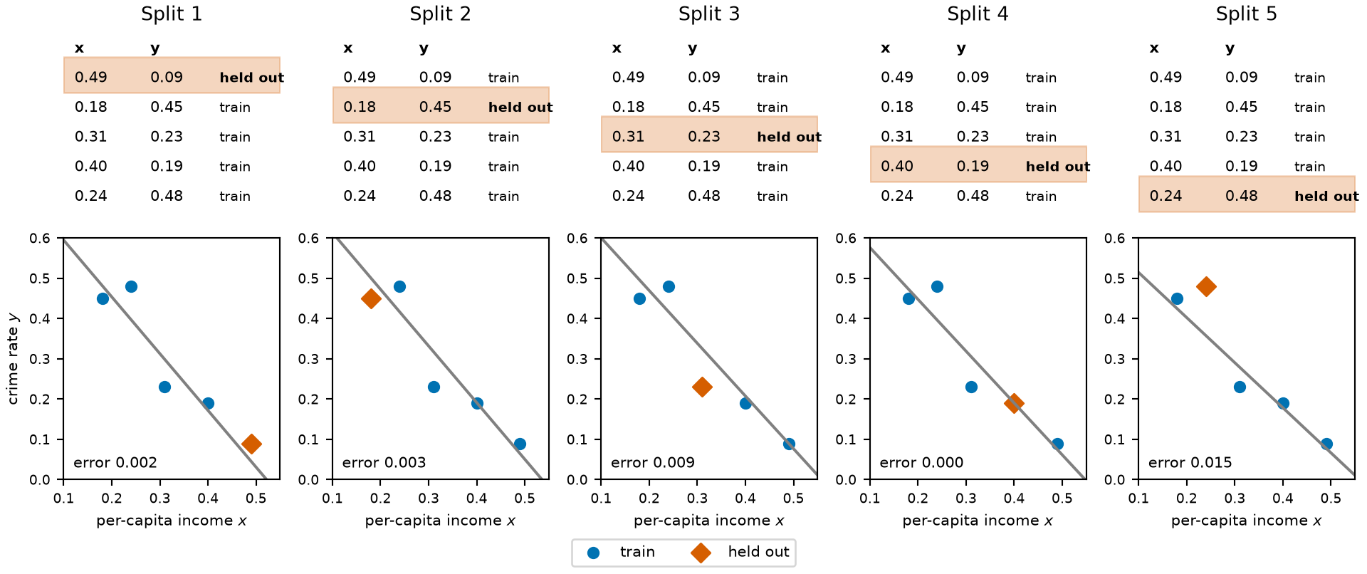
The five squared errors are 0.002, 0.003, 0.009, 0.000, 0.015, and their mean, the leave-one-out estimate of the risk, is \(0.006\), with a 95% confidence interval of \(-0.002\) to \(0.013\). The interval is wide because five errors say little about their mean, and it is not a valid interval: the five errors share training points, so they are not independent, and squared errors are skewed, so a t interval fits them poorly. It reaches below zero, which a mean of squared errors cannot, so treat it as a rough guide to the uncertainty. Every neighborhood is scored once, by a line that never saw it, and every neighborhood helps fit four of the five lines. The largest error, 0.015, is in split 5, and the next largest, 0.009, is in split 3. Those two neighborhoods have incomes 0.24 and 0.31, on either side of the steep drop in crime rate that a straight line fitted without one of them smooths over.
Watch
Hutchinson covers train, dev and test sets and cross-validation, Generalization, part 2 (11 min) [3]. The chapter Model Selection puts its cross-validation videos beside each method.
Watch
Starmer explains cross-validation [10].
Read
GeeksforGeeks explains cross-validation [11].
Show code
# The constants of this figure live here, so the widget, the static plot and the prose agree.
cv_n <- 40          # points drawn, and so held-out squared errors
cv_k <- 5           # folds of the static plot
cv_degree <- 3      # degree of the static plot
cv_fresh_n <- 2000  # fresh points the static plot scores
cv_sd <- 0.1        # standard deviation of the noise in the static plot
Show code
cvSplit = biCarSplit(cvN, 3100 + cvDraw)
cvData = cvSplit.train
cvHeld = cvSplit.held
// Deal the points into k folds at random: shuffle, then fold = position mod k.
cvFold = {
  const order = d3.shuffler(d3.randomLcg(4100 + cvDraw))(d3.range(cvN));
  const fold = new Array(cvN);
  order.forEach((i, pos) => { fold[i] = pos % cvK; });
  return fold;
}
// The k-fold estimate for one degree: fit on k - 1 folds, score the one left out.
cvScore = (degree) => {
  const sq = [];
  const perFold = d3.range(cvK).map((f) => {
    const train = cvData.filter((_, i) => cvFold[i] !== f);
    const test = cvData.filter((_, i) => cvFold[i] === f);
    const h = biPolyfit(train, degree);
    // Every point is scored exactly once, by the fit that left it out.
    test.forEach(([x, y]) => sq.push((h(x) - y) ** 2));
    return {fold: f + 1, rmse: biRmse(h, test)};
  });
  // The k-fold estimate of the RMSE is the root of the average of the fold MSEs,
  // which is the root of the mean of all n held-out squared errors when the folds are equal.
  // Its interval is the bootstrap interval for that mean of squared errors, square-rooted.
  // It is approximate: the n errors are not independent, since each fit shares most of its
  // training points with the others, so the true interval is somewhat wider (see the caption).
  const ci = biRmseCIBoot(sq, 7);
  return {perFold, mean: Math.sqrt(d3.mean(perFold, (d) => d.rmse ** 2)), ci};
}
cvNow = cvScore(cvDegree)
// For comparison: the model fitted to all cvN cars, scored on the other cars.
cvFresh = (degree) => biRmse(biPolyfit(cvData, degree), cvHeld)
cvFreshCI = (degree) => biRmseCI(biPolyfit(cvData, degree), cvHeld)
cvCurve = d3.range(0, 9).flatMap((degree) => {
  const score = cvScore(degree);
  const fresh = cvFreshCI(degree);
  // Each series is drawn a little to one side of the degree, so the two bars do not overlap.
  return [
    {degree, x: degree - 0.1, what: "k-fold estimate", rmse: biMpgUnits(score.mean),
     lo: Math.max(biMpgUnits(score.ci.lo), 1e-1), hi: biMpgUnits(score.ci.hi)},
    {degree, x: degree + 0.1, what: "error on fresh points", rmse: biMpgUnits(fresh.mean),
     lo: Math.max(biMpgUnits(fresh.lo), 1e-1), hi: biMpgUnits(fresh.hi)}
  ];
})
// One row per fold, one column per point (sorted by x): scored or trained on.
cvCells = {
  const byX = d3.sort(d3.range(cvN), (i) => cvData[i][0]);
  return d3.range(cvK).flatMap((f) => byX.map((i, col) => ({
    fold: f + 1, col: col + 1, role: cvFold[i] === f ? "scored" : "trained on"
  })));
}
Change \(k\) and the degree in Figure 5, and compare the \(k\)-fold estimate with the error on fresh points.
Show code
Show code
md`${cvK} fits, each on ${cvN - cvN / cvK} points and scored on the other ${cvN / cvK}.
The RMSE on each held-out fold, in mpg, is ${cvNow.perFold.map((d) => `${d.fold}: ${biMpgUnits(d.rmse).toFixed(2)}`).join("; ")}.
The overall ${cvK}-fold cross-validation RMSE for degree ${cvDegree} is **${biMpgUnits(cvNow.mean).toFixed(2)} mpg**,
with an approximate 95% confidence interval of ${biFmtCIMpg(cvNow.ci)};
the degree-${cvDegree} fit to all ${cvN} points scores **${biMpgUnits(cvFresh(cvDegree)).toFixed(2)} mpg** on the other ${cvHeld.length} cars,
with a 95% confidence interval of ${biFmtCIMpg(cvFreshCI(cvDegree))}.`
Show code
Plot.plot({
  ariaLabel: 'The fold assignment as a grid: one row per fold, the fit that leaves it out, ' +
    'one column per data point sorted by x, ' +
    'each cell orange where that fit scores the point and light blue where it trains on it.',
  width: 320, height: Math.min(40 + 14 * cvK, 200), marginLeft: 40,
  x: {label: "data point, sorted by x", ticks: []},
  y: {label: "fold", ticks: cvK <= 10 ? d3.range(1, cvK + 1) : [1, 5, 10, 15, 20]},
  color: {domain: ["trained on", "scored"], range: ["#c6dbef", "#ff7f0e"], legend: true},
  marks: [
    Plot.cell(cvCells, {x: "col", y: "fold", fill: "role", inset: 0.5})
  ]
})
Show code
{
// A log axis spanning whole powers of ten around everything drawn,
// so that its power-of-ten ticks all fall inside it.
// `shown` holds the k fold scores, then their mean, then the fresh-point error,
// converted to miles per gallon and floored at 1e-6 because a log scale cannot place a zero.
const shown = [...cvNow.perFold.map((d) => d.rmse), cvNow.mean, cvFresh(cvDegree),
  cvNow.ci.lo, cvNow.ci.hi].map((v) => Math.max(biMpgUnits(v), 1e-6));
const yDomain = [10 ** Math.floor(Math.log10(d3.min(shown))), 10 ** Math.ceil(Math.log10(d3.max(shown)))];
return Plot.plot({
  ariaLabel: 'The root mean squared error on each held-out fold as a dot, ' +
    'with a solid line at their root-mean-square, the k-fold estimate, ' +
    'a pale band for its approximate 95% confidence interval, ' +
    'and a dashed line at the error on fresh points.',
  width: 320, height: 150, marginLeft: 50, grid: true,
  x: {label: "fold", ticks: cvK <= 10 ? d3.range(1, cvK + 1) : [1, 5, 10, 15, 20],
      tickFormat: "d"},
  y: {type: "log", domain: yDomain, label: "fold RMSE (mpg, log scale)",
      ticks: biPow10(...yDomain), tickFormat: biExp},
  marks: [
    // The approximate 95% confidence interval of the k-fold estimate, as a pale band.
    Plot.rectY([{lo: shown[cvK + 2], hi: shown[cvK + 3]}],
      {x1: 0.5, x2: cvK + 0.5, y1: "lo", y2: "hi", fill: "#ff7f0e", fillOpacity: 0.2}),
    Plot.ruleY([shown[cvK]], {stroke: "#ff7f0e", strokeWidth: 2}),
    Plot.ruleY([shown[cvK + 1]], {stroke: "#222", strokeDasharray: "5,4"}),
    Plot.dot(cvNow.perFold, {x: "fold", y: (_, i) => shown[i], r: 4, fill: "#ff7f0e"})
  ]
});
}
Show code
Plot.plot({
  ariaLabel: 'The k-fold estimate and the error on fresh points, ' +
    'against polynomial degree from 0 to 8, on a log scale, ' +
    'with a 95% confidence interval drawn around each error, ' +
    'and the chosen degree marked by a vertical line.',
  width: 320, height: 200, marginLeft: 50, grid: true,
  x: {domain: [-0.4, 8.4], label: "degree", ticks: d3.range(0, 9)},
  y: {type: "log", domain: [1e-1, 1e2], clamp: true, label: "RMSE (mpg, log scale)",
      ticks: biPow10(1e-1, 1e2), tickFormat: biExp},
  color: {domain: ["k-fold estimate", "error on fresh points"], range: ["#ff7f0e", "#222"],
          legend: true},
  marks: [
    Plot.ruleX([cvDegree], {stroke: "#888"}),
    // The 95% confidence interval of each error, as a vertical bar.
    Plot.ruleX(cvCurve, {x: "x", y1: "lo", y2: "hi", stroke: "what", strokeWidth: 1.5}),
    Plot.line(cvCurve, {x: "x", y: "rmse", stroke: "what", strokeWidth: 2}),
    Plot.dot(cvCurve, {x: "x", y: "rmse", fill: "what", r: 3})
  ]
})Remark 8 (Cross-validation replaces the validation set)
Remark 8 (Cross-validation replaces the validation set). Used to choose between models, cross-validation takes the place of the validation set, the one used again and again, and not of the final test set, which stays unused. Whichever scheme picked the model, the data used to pick it cannot also be the data used to report how good it is. If cross-validation picks the polynomial degree in Figure 5, for example, the cross-validation error of the winning degree is optimistic, because that degree won partly by fitting this sample’s noise well; an honest estimate needs points that took no part in the choice.
Reading
Starmer [13] covers the fundamental concepts of machine learning and cross-validation with pictures and little algebra.
Stanford University [14], Lectures 3–6, are handwritten notes from a Stanford course on probability and inference. They cover concentration inequalities (Hoeffding’s inequality in Lecture 3), empirical risk minimization and overfitting (Lecture 5), and uniform convergence with generalization bounds (Lecture 6), for readers who want the mathematics behind Hoeffding’s inequality in more detail. The textbook these notes recommend for this material is Shalev-Shwartz and Ben-David [15], Sections 2.1–2.3 and 4.1–4.2, which is free online.
Watch
Andrew Ng’s short lecture for DeepLearning.AI explains how to split data into a training set, a validation set and a test set [16]. The lecture calls the validation set the “dev set”.
Dependency graph
Open the block to see every definition and result of this page, with prerequisites at the top. Click a box to jump to it.