Gradient Descent
Last modified: 2026-10-28
Source
Consolidated from two sources, each of which introduces gradient descent as a digression within its logistic regression material: Kameron Decker Harris’ 2022 handwritten lecture notes, whose Week 6 contains most of it, and Brian Hutchinson’s Fall 2025 lecture notes, reproduced in Logistic Regression, which is the fuller of the two on line search — it is where both hyperparameters \(b \in (0,1)\) and \(\armijo \in (0, 0.5]\) come from. Two separate copies of one digression is the argument for pulling it out: many models after Linear Regression are fitted this way, so the optimizer deserves its own treatment rather than being re-derived in each chapter that needs it.
The source notes’ regularized stochastic step is corrected in Solution 83; the correction is flagged there rather than applied silently.
1 Why an iterative method
Linear Regression computes its fitted model from a closed-form solution. Set the gradient of the squared-error cost to zero, and the resulting normal equations are linear in \(\vcoef\). When \(X^\top X\) is invertible, one matrix solve produces the exact minimizer, the closed form \(\hvcoef = (X^\top X)^{-1} X^\top \vy\). Ridge regression has a closed-form solution of the same kind. Few other models in this course have one.
These models have costs whose minimizer has no closed-form solution:
What we have instead is the ability to evaluate the cost at a point, and to evaluate its gradient there. Gradient descent is the algorithm that turns those two abilities into a fit.
Exercise 1 (Why we cannot always just solve for \(\vcoef\))
Exercise 1 (Why we cannot always just solve for \(\vcoef\)) Least squares has a closed-form solution: set the gradient to zero, and the resulting normal equations \((\stprod{\design})\vcoef = \tp{\design} \vy\) are linear in \(\vcoef\), so when \(\stprod{\design}\) is invertible one matrix solve gives the answer.
Say precisely which feature of the squared-error cost makes its gradient linear in \(\vcoef\).
Solution 1. The squared-error cost is a quadratic in \(\vcoef\): every appearance of \(\vcoef\) is inside \(\dprod{\vcoef}{\vx_i}\), and that term is squared and nothing more. Differentiating a quadratic drops the degree by one, so the gradient is affine in \(\vcoef\), and setting an affine function to zero is a linear system.
Exercise 2 (Why we cannot always just solve for \(\vcoef\) (part 2))
Exercise 2 (Why we cannot always just solve for \(\vcoef\) (part 2)) Use the setup of Exercise 1.
Logistic regression minimizes \[C(\vcoef) = \sumin \sb{-y_i \log \sigmoid(\dprod{\vcoef}{\vx_i}) - (1-y_i)\log\paren{1 - \sigmoid(\dprod{\vcoef}{\vx_i})}}\] where \(\sigmoid(z) = 1/(1 + \e{-z})\) is the logistic (sigmoid) function, which logistic regression introduces in full. The gradient is \(\grad C = \sumin \paren{\sigmoid(\dprod{\vcoef}{\vx_i}) - y_i}\vx_i\). Set that to zero and explain why the same step fails.
Solution 2. The score equations are
\[\sumin \paren{\sigmoid(\dprod{\vcoef}{\vx_i}) - y_i}\vx_i = \vzero\]
The unknown \(\vcoef\) sits inside \(\sigmoid(z) = 1/(1 + e^{-z})\), so each equation is a sum of exponentials of \(\vcoef\) rather than a linear combination of its entries. There is no rearrangement that isolates \(\vcoef\) on one side: the system is non-linear, and \(\ninputvars+1\) non-linear equations in \(\ninputvars+1\) unknowns have no general solution formula. The cost is still convex, which rules out spurious local minima, but convexity alone does not deliver a minimizer. The logistic loss is strictly convex in the fitted scores \(\design\vcoef\) rather than in \(\vcoef\), so uniqueness needs \(\design\) to have full column rank, and existence needs the classes not to be perfectly separable — otherwise the cost keeps falling as \(\norm{\vcoef}\) grows and no finite minimizer exists at all. Given both, the minimizer is unique, and we simply have no way to write it down. Finding it is a search, which is the subject of the rest of this chapter.
Exercise 3 (Why we cannot always just solve for \(\vcoef\) (part 3))
Exercise 3 (Why we cannot always just solve for \(\vcoef\) (part 3)) Use the setup of Exercise 1.
Give a second reason to fit iteratively that has nothing to do with non-linearity, and applies even to plain least squares.
Solution 3. Size. Forming \(\stprod{\design}\) costs \(O(n\ninputvars^2)\) and inverting it costs \(O(\ninputvars^3)\), and both require the whole of \(\design\) to be available at once. With \(\ninputvars\) in the thousands the cube dominates, and with \(n\) in the hundreds of millions the data does not fit in memory at all. A gradient step needs only \(O(n\ninputvars)\) work — or, as Solution 71 shows, only \(O(\ninputvars)\) — and can be taken while the data streams past. So an iterative method is the answer both to we cannot solve it and to we cannot afford to solve it.
Watch
Andrew Ng introduces gradient descent in the second CS229 lecture, from 18:06 [1], Lecture 2.
Exercise 4 (Is an argmin an algorithm?)
Exercise 4 (Is an argmin an algorithm?) A squared-error objective is an expression in \(\vcoef\), and gradient descent is an algorithm that minimizes it. Math for Data Science asks how the two differ for a polynomial.
Now take a general cost function \(C(\vcoef)\), not only squared error. Can you turn \(\argmin_{\vcoef} C(\vcoef)\) into a list of steps that returns the minimizing \(\vcoef\) exactly?
Solution 4. Not in general. Only for special costs, such as the squared error of linear regression, does a formula exist, and evaluating that formula is an algorithm. For other costs, such as the logistic cost of Exercise 2, the argmin is a well-defined value that no formula returns. We choose an algorithm that approximates it.
Example 1 (An argmin with no closed-form expression)
Example 1 (An argmin with no closed-form expression) The logistic cost \(C(\vcoef)\) of Exercise 2 is an expression, and \(\hvcoef = \argmin_{\vcoef} C(\vcoef)\) is a well-defined vector, but no closed-form expression returns it. Gradient descent is an algorithm that supplies steps approaching it.
2 The descent direction
At a given \(\vcoef_t\), we want to move so that the cost goes down. The gradient
\[\grad_{\vcoef} C(\vcoef) = \sbmat{ \partial C / \partial \coef{0} \\ \partial C / \partial \coef{1} \\ \vdots \\ \partial C / \partial \coef{\ninputvars} }\]
collects the partial derivatives, so it says how fast \(C\) rises in each coordinate direction. It also says more than that: it identifies the single direction of fastest increase, and therefore its negative is the direction of fastest decrease.
Exercise 5 (Show that the negative gradient is the steepest direction)
Exercise 5 (Show that the negative gradient is the steepest direction) “Go downhill” does not by itself say which way. This exercise shows that the negative gradient is the best answer, and says what “best” means here.
Write the first-order Taylor expansion of \(C(\vcoef + \smallconst\vu)\) about \(\vcoef\), for a small scalar \(\smallconst > 0\) and a direction \(\vu\) with \(\norm{\vu}_2 = 1\).
Solution 5. \[C(\vcoef + \smallconst\vu) = C(\vcoef) + \smallconst\, \dprod{\vu}{\grad C(\vcoef)} + O(\smallconst^2)\]
Exercise 6 (Show that the negative gradient is the steepest direction (part 2))
Exercise 6 (Show that the negative gradient is the steepest direction (part 2)) Use the setup of Exercise 5.
Which term in that expansion depends on \(\vu\)? Making the step as downhill as possible therefore means minimizing that term over all unit \(\vu\).
Solution 6. Only the middle term. \(C(\vcoef)\) is fixed at the current point, and the remainder shrinks faster than \(\smallconst\) as the step shrinks, so for a short enough step the sign and size of the change are decided by \(\dprod{\vu}{\grad C}\) alone.
Exercise 7 (Show that the negative gradient is the steepest direction (part 3))
Exercise 7 (Show that the negative gradient is the steepest direction (part 3)) Use the setup of Exercise 5.
State the Cauchy–Schwarz inequality, including the condition for equality, and use it to find the minimizing \(\vu\).
Solution 7. Cauchy–Schwarz says \(|\va^\top \v{b}| \le\norm{\va}_2\norm{\v{b}}_2\), with equality exactly when \(\va\) and \(\v{b}\) are parallel — one is a scalar multiple of the other.
With \(\norm{\vu}_2 = 1\) this gives
\[-\norm{\grad C}_2 \;\le\; \dprod{\vu}{\grad C} \;\le\;\norm{\grad C}_2\]
The lower bound is attained when \(\vu\) is parallel to \(\grad C\) and the inner product is negative, which determines \(\vu\) uniquely:
\[\vu^\star = -\frac{\grad C}{\norm{\grad C}_2}\]
and then \(\dprod{\vu^\star}{\grad C} = -\norm{\grad C}_2\). This is the same geometry as Linear functions as inner products: \(\dprod{\vu}{\grad C} =\norm{\grad C}_2\cos\angpar\), minimized at \(\angpar = 180^\circ\).
Exercise 8 (Show that the negative gradient is the steepest direction (part 4))
Exercise 8 (Show that the negative gradient is the steepest direction (part 4)) Use the setup of Exercise 5.
The gradient of \(C\) at that point is \(\grad C = (3, -4)^\top\). Write the unit step direction, and say how much \(C\) falls per unit of step length, to first order.
Solution 8. \(\norm{\grad C}_2 = \sqrt{9 + 16} = 5\), so
\[ \begin{aligned} \vu^\star &= -\tfrac{1}{5}(3, -4)^\top \\ &= (-0.6,\, 0.8)^\top \end{aligned} \]
and \(C\) falls at rate \(\norm{\grad C}_2 = 5\) per unit of step length, to first order. Note that the rate is the length of the gradient, while the direction is the gradient normalized. Both come out of the same inequality.
Exercise 9 (Show that the negative gradient is the steepest direction (part 5))
Exercise 9 (Show that the negative gradient is the steepest direction (part 5)) Use the setup of Exercise 5.
Name two things this argument does not establish.
Solution 9. Two things, and both matter for the rest of the chapter.
It is local. The expansion is only accurate for small \(\smallconst\), so “steepest” describes the slope at the current point and says nothing about where the step lands. A direction that starts out steepest can be overtaken within the very same step, which is exactly why the step size needs its own treatment in Choosing the step size.
It depends on the norm. The constraint was \(\norm{\vu}_2 = 1\). Measure the unit step with a different norm and a different direction wins: under \(\norm{\vu}_\infty = 1\) the steepest direction is \(-\sign(\grad C)\), which is the sign-of-the-gradient rule some optimizers use. So “the steepest descent direction” is a statement about the geometry we imposed, not a property of \(C\) on its own.
Watch
Weinberger derives the descent direction from a local approximation of the cost, from 13:30 [2], Lecture 12.
3 The algorithm
The math notes define gradient descent, and this chapter uses it as stated there. Here the cost is \(C\), the parameter vector is \(\vcoef\), and each step is scaled by \(\learnrate\). In this notation, the update at step \(t\) is
\[\vcoef_{t} = \vcoef_{t-1} - \learnrate\,\grad_{\vcoef} C(\vcoef_{t-1}).\]
The algorithm repeats this update until it has converged. Three things in the update have to be chosen, and each gets its own section:
- where to start;
- how long a step to take;
- when to stop.
Definition 1 (Learning rate)
Definition 1 (Learning rate) The learning rate \(\learnrate > 0\) of gradient descent is the number that multiplies the gradient in each update. It is also called the step size.
Example 2 (One step at two learning rates)
Example 2 (One step at two learning rates) Let:
- \(C(\regcoef) = \regcoef^2\) be the cost, with derivative \(C'(\regcoef) = 2\regcoef\);
- \(\regcoef_0\) be the starting value of \(\regcoef\);
- \(\learnrate_{\text{small}}\) and \(\learnrate_{\text{large}}\) be the two learning rates to compare.
Start at \(\regcoef_0 = 2\), so \(C'(\regcoef_0) = 4\). The first update is \(\regcoef_1 = \regcoef_0 - 4\,\learnrate\):
- for \(\learnrate_{\text{small}} = 0.25\), \(\regcoef_1 = 1\), which is closer to the minimizer \(0\);
- for \(\learnrate_{\text{large}} = 1.25\), \(\regcoef_1 = -3\), which is farther from \(0\) than the start was.
A larger learning rate moves farther, but too far overshoots the minimizer.
Definition 2 (Gradient flow)
Definition 2 (Gradient flow) Let \(C\) be the cost. Gradient flow is the curve \(\vcoef(t)\) that solves the differential equation
\[\dif{\vcoef(t)}{t} = -\grad C(\vcoef(t)).\]
Gradient descent is Euler’s method for this equation, with the learning rate \(\learnrate\) as the step in \(t\). The flow runs downhill, perpendicular to the level sets.
Example 3 (Gradient descent follows the flow)
Example 3 (Gradient descent follows the flow) Let:
- \(C(\regcoef) = \tfrac{1}{2}\regcoef^2\) be the cost, so \(\grad C(\regcoef) = \regcoef\);
- \(\regcoef_0\) be the starting value of \(\regcoef\);
- \(T\) be the time at which to compare the two paths.
The gradient flow solves \(\dif{\regcoef(t)}{t} = -\regcoef(t)\), and its solution is \(\regcoef(t) = \regcoef_0\,\expf{-t}\). Gradient descent with learning rate \(\learnrate\) multiplies \(\regcoef\) by \(1 - \learnrate\) at each step, so after \(k\) steps it has reached time \(t = k\learnrate\) with \(\regcoef_k = \regcoef_0 (1 - \learnrate)^k\).
Start at \(\regcoef_0 = 1\) and run to time \(T = 1\):
- for \(\learnrate = 0.5\), \(\regcoef_{2} = 0.25\);
- for \(\learnrate = 0.01\), \(\regcoef_{100} = 0.366\);
- the flow gives \(\regcoef(T) = 0.3679\).
The smaller the learning rate, the closer the descent stays to the flow.
Exercise 10 (Take one step by hand, three times)
Exercise 10 (Take one step by hand, three times) Use the three points of Solve the normal equations by hand:
\[(x_1, y_1) = (0, 1), \quad (x_2, y_2) = (1, 3), \quad (x_3, y_3) = (2, 3)\]
so that, with the intercept trick,
\[\design = \sbmat{ 1 & 0 \\ 1 & 1 \\ 1 & 2 }, \qquad \vy = \sbmat{ 1 \\ 3 \\ 3 }, \qquad J(\vcoef) =\norm{\design\vcoef - \vy}_2^2\]
Start from \(\vcoef_0 = (0,0)^\top\) and work in exact fractions.
Compute \(J(\vcoef_0)\) and \(\grad J(\vcoef_0)\).
Solution 10. At \(\vcoef_0 = \vzero\) the fitted values are all zero, so the residual is \(\design\vcoef_0 - \vy = (-1, -3, -3)^\top\) and
\[ \begin{aligned} J(\vcoef_0) &= 1 + 9 + 9 \\ &= 19 \end{aligned} \]
Using \(\grad J = 2\tp{\design}(\design\vcoef - \vy)\) from The gradient,
\[\tp{\design} \sbmat{ -1 \\ -3 \\ -3 } = \sbmat{ -1-3-3 \\ 0-3-6 } = \sbmat{ -7 \\ -9 }, \qquad \grad J(\vcoef_0) = \sbmat{ -14 \\ -18 }\]
The gradient is negative in both coordinates, so both the intercept and the slope should increase — which is right, since the data sits above and to the right of the origin.
Exercise 11 (Take one step by hand, three times (part 2))
Exercise 11 (Take one step by hand, three times (part 2)) Use the setup of Exercise 10.
Take one step \(\vcoef_1 = \vcoef_0 - \learnrate\grad J(\vcoef_0)\) for each of \(\learnrate = \tfrac{1}{20}\), \(\learnrate = \tfrac{1}{10}\) and \(\learnrate = \tfrac{3}{20}\), and compute \(J(\vcoef_1)\) in each case.
Solution 11. Each step is \(\vcoef_1 = -\learnrate\,(-14, -18)^\top = \learnrate\,(14, 18)^\top\).
| \(\learnrate\) | \(\vcoef_1\) | fitted values | residual | \(J(\vcoef_1)\) |
|---|---|---|---|---|
| \(1/20\) | \((7/10,\ 9/10)\) | \((7/10,\ 16/10,\ 25/10)\) | \((-3/10,\ -14/10,\ -5/10)\) | \(23/10 = 2.30\) |
| \(1/10\) | \((7/5,\ 9/5)\) | \((7/5,\ 16/5,\ 5)\) | \((2/5,\ 1/5,\ 2)\) | \(21/5 = 4.20\) |
| \(3/20\) | \((21/10,\ 27/10)\) | \((21/10,\ 48/10,\ 75/10)\) | \((11/10,\ 18/10,\ 45/10)\) | \(247/10 = 24.70\) |
Exercise 12 (Take one step by hand, three times (part 3))
Exercise 12 (Take one step by hand, three times (part 3)) Use the setup of Exercise 10.
Solve the normal equations by hand found the minimizer \(\vcoef^\star = (4/3, 1)^\top\) with \(J(\vcoef^\star) = 2/3\). Which of the three steps moved downhill?
Solution 12. The first two moved downhill: \(2.30\) and \(4.20\) are both below \(19\). The third went up, from \(19\) to \(24.70\).
Exercise 13 (Take one step by hand, three times (part 4))
Exercise 13 (Take one step by hand, three times (part 4)) Use the setup of Exercise 10.
Which of the three steps got closest to the minimizer \(\vcoef^\star\)?
Solution 13. The closest to \(\vcoef^\star = (4/3, 1) \approx (1.333, 1.000)\) is \(\learnrate = 1/20\), at \((0.7, 0.9)\), a distance of about \(0.64\). The \(\learnrate = 1/10\) step lands at \((1.4, 1.8)\), distance about \(0.80\): it has overshot in the slope while the intercept is nearly right. The \(\learnrate = 3/20\) step lands at \((2.1, 2.7)\), distance about \(1.87\), further from the answer than where it started.
Note that \(J\) and distance-to-\(\vcoef^\star\) order the three steps the same way here, but they are different quantities and will not always agree.
Exercise 14 (Take one step by hand, three times (part 5))
Exercise 14 (Take one step by hand, three times (part 5)) Use the setup of Exercise 10.
One of the three raised the cost. Nothing about the direction was wrong. Say what went wrong instead.
Solution 14. The step was too long. The direction \(-\grad J\) is downhill, as Solution 7 proved, but only over a short enough step — the Taylor expansion that justified it drops an \(O(\smallconst^2)\) term, and at \(\learnrate = 3/20\) that term is no longer small. Geometrically, the step crosses the valley and ends at a higher cost than it started.
The direction is free to choose and always correct. The length is the part that has to be chosen carefully, and Choosing the step size makes the boundary exact: for this \(\design\), any \(\learnrate < 0.1396\) shrinks the error and any \(\learnrate > 0.1396\) grows it. So \(3/20 = 0.15\) failed and \(1/10\) did not.
Definition 3 (Rosenbrock function)
Definition 3 (Rosenbrock function) The Rosenbrock function on \(\reals^2\) is
\[f(\vx) = 100\paren{x_2 - x_1^2}^2 + \paren{1 - x_1}^2, \qquad \vx = \tp{(x_1, x_2)}.\]
It is a standard test problem for optimizers [3].
Example 4 (Values of the Rosenbrock function)
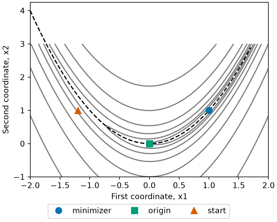
Example 4 (Values of the Rosenbrock function) Evaluate the function at the minimizer \((1, 1)\), at the origin, and at the standard starting point \((-1.2, 1)\). Then evaluate it along the curve \(x_2 = x_1^2\), which the function treats as the floor of a narrow, curved valley:
{'minimizer': 0, 'origin': 1, 'start': 24.2}[4. 1. 0.25 0. 1. ] [4. 1. 0.25 0. 1. ]minimizer origin start
0.0 1.0 24.2 [,1] [,2] [,3] [,4] [,5]
on_curve 4 1 0.25 0 1
formula 4 1 0.25 0 1The function is \(0\) at \((1, 1)\) and positive everywhere else, so \((1, 1)\) is the global minimizer. At the starting point the value is 24.2, mostly from the first term, because \((-1.2, 1)\) is off the curve \(x_2 = x_1^2\). On the curve the function is small and varies slowly, so the valley floor is nearly flat even though its walls are steep.
Show code
library(ggplot2)
rf_grid <- expand.grid(x1 = seq(-2, 2, length.out = 201), x2 = seq(-1, 3, length.out = 201))
rf_grid$f <- rosenbrock_rf(rf_grid$x1, rf_grid$x2)
rf_points <- data.frame(
  name = names(points_rf),
  x1 = sapply(points_rf, `[`, 1),
  x2 = sapply(points_rf, `[`, 2)
)
rf_curve <- data.frame(x1 = seq(-2, 1.7, length.out = 200))
rf_curve$x2 <- rf_curve$x1^2
ggplot(rf_grid, aes(x1, x2)) +
  geom_contour(aes(z = f), colour = "grey60", breaks = c(1, 3, 10, 30, 100, 300, 1000)) +
  geom_line(data = rf_curve, linetype = "dashed") +
  geom_point(aes(colour = name, shape = name), data = rf_points, size = 3) +
  scale_colour_manual(values = c(minimizer = "#0072B2", origin = "#009E73", start = "#D55E00")) +
  scale_shape_manual(values = c(minimizer = 16, origin = 15, start = 17)) +
  coord_cartesian(xlim = c(-2, 2), ylim = c(-1, 3)) +
  labs(x = "First coordinate, x1", y = "Second coordinate, x2", colour = NULL, shape = NULL)
Show code
import matplotlib.pyplot as plt
import numpy as np

g1_rf, g2_rf = np.meshgrid(np.linspace(-2, 2, 201), np.linspace(-1, 3, 201))
fig, ax = plt.subplots(figsize=(5, 4), layout="constrained")
ax.contour(g1_rf, g2_rf, rosenbrock_rf(g1_rf, g2_rf), levels=[1, 3, 10, 30, 100, 300, 1000], colors="grey");
t_rf = np.linspace(-2, 1.7, 200)
ax.plot(t_rf, t_rf ** 2, color="black", linestyle="--");
style_rf = {"minimizer": ("#0072B2", "o"), "origin": ("#009E73", "s"), "start": ("#D55E00", "^")}
for name, p in points_rf.items():
    ax.plot(*p, color=style_rf[name][0], marker=style_rf[name][1], linestyle="", markersize=8, label=name);
ax.set_xlabel("First coordinate, x1");
ax.set_ylabel("Second coordinate, x2");
fig.legend(loc="outside lower center", ncol=3);
plt.show()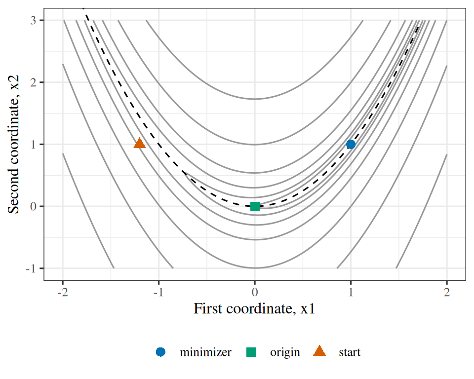
Exercise 15 (Descend the Rosenbrock function)
Exercise 15 (Descend the Rosenbrock function) Use Definition 3.
Compute the gradient \(\grad f(\vx)\).
Solution 15. Differentiate each term with the chain rule. The first term depends on both coordinates:
\[ \begin{aligned} \deriv{x_1}\, 100\paren{x_2 - x_1^2}^2 &= 200\paren{x_2 - x_1^2} \cdot \paren{-2x_1} \\ &= -400\, x_1 \paren{x_2 - x_1^2}, \end{aligned} \]
\[ \deriv{x_2}\, 100\paren{x_2 - x_1^2}^2 = 200\paren{x_2 - x_1^2}. \]
The second term depends only on \(x_1\): \(\deriv{x_1}\paren{1 - x_1}^2 = -2\paren{1 - x_1}\). So
\[ \grad f(\vx) = \sbmat{ -400\, x_1 \paren{x_2 - x_1^2} - 2\paren{1 - x_1} \\ 200\paren{x_2 - x_1^2} }. \]
Exercise 16 (Descend the Rosenbrock function (part 2))
Exercise 16 (Descend the Rosenbrock function (part 2)) Use the setup of Exercise 15.
Write the gradient descent update \(\vx_{k+1}\) with step size \(\learnrate\) as a pair of formulas in \(x_{k,1}\) and \(x_{k,2}\).
Solution 16. Subtracting \(\learnrate\) times the gradient from \(\vx_k\), coordinate by coordinate:
\[ \begin{aligned} x_{k+1,1} &= x_{k,1} + \learnrate\paren{400\, x_{k,1}\paren{x_{k,2} - x_{k,1}^2} + 2\paren{1 - x_{k,1}}}, \\ x_{k+1,2} &= x_{k,2} - 200\, \learnrate\paren{x_{k,2} - x_{k,1}^2}. \end{aligned} \]
Exercise 17 (Descend the Rosenbrock function (part 3))
Exercise 17 (Descend the Rosenbrock function (part 3)) Use the setup of Exercise 15.
Check the gradient numerically at \(\vx = \tp{(-1.2, 1)}\) against a finite-difference approximation of each partial derivative.
Solution 17.
# The Rosenbrock function and its gradient from part 1.
rosenbrock <- function(x) {
  100 * (x[2] - x[1]^2)^2 + (1 - x[1])^2
}
rosenbrock_grad <- function(x) {
  c(
    -400 * x[1] * (x[2] - x[1]^2) - 2 * (1 - x[1]),
    200 * (x[2] - x[1]^2)
  )
}

# Central finite differences, one coordinate at a time, as an
# independent check on the formula: it does not use the derivation.
x0 <- c(-1.2, 1)
eps <- 1e-6
fd_grad <- vapply(
  1:2,
  function(j) {
    e <- replace(numeric(2), j, eps)
    (rosenbrock(x0 + e) - rosenbrock(x0 - e)) / (2 * eps)
  },
  numeric(1)
)
grad_gap <- max(abs(fd_grad - rosenbrock_grad(x0)))
The largest gap between the formula and the finite differences is 2.2e-08, which is finite-difference error, so the gradient agrees with the numerical derivative.
Exercise 18 (Descend the Rosenbrock function (part 4))
Exercise 18 (Descend the Rosenbrock function (part 4)) Use the setup of Exercise 15.
Run 1000 steps with \(\learnrate = 0.001\) from \(\vx_0 = \tp{(-1.2, 1)}\).
Exercise 19 (Descend the Rosenbrock function (part 5))
Exercise 19 (Descend the Rosenbrock function (part 5)) Use the setup of Exercise 15.
Is the final iterate close to the minimizer of \(f\)?
Solution 19. The function is zero at \(\tp{(1, 1)}\) and positive everywhere else, so \(\tp{(1, 1)}\) is the minimizer. After 1000 steps the iterate is \(\tp{(0.327, 0.104)}\) and \(f\) has fallen from 24.2 to 0.454. That is progress, but the iterate is not close to \(\tp{(1, 1)}\). The minimizer sits at the end of a long, curved, narrow valley, the same shape that Solution 38 describes for a badly conditioned least squares problem, and a step size small enough not to bounce off the valley walls advances only slowly along its floor.
Watch
Andrew Ng writes the algorithm out in the second CS229 lecture, from 33:01 [1], Lecture 2.
Watch
Hutchinson covers gradient descent, step size and learning rate (15 min) [5]. The video site requires a login, which enrolled students find in the syllabus.
Read
GeeksforGeeks explains gradient descent [6].
Read
The University of Washington’s CSE 446 slides cover gradient descent, convexity and the theory of gradient descent [7], Lectures 9 to 11.
4 Convexity and stationary points
Whether descent can be trusted depends on the shape of the cost \(J\). The definitions of a convex function, a stationary point, a local minimizer, a local maximizer and a saddle point are in the math notes, and are used here as they are stated there. This section adds an example for each idea.
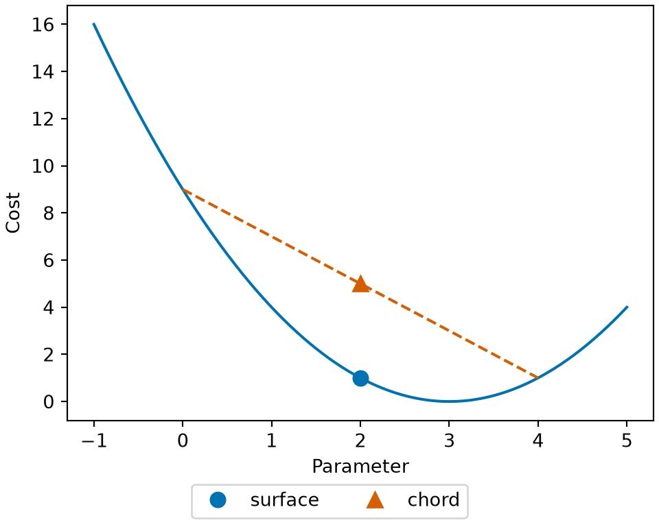
Example 5 Take the one-parameter squared-error cost \(J(\regcoef) = (\regcoef - 3)^2\), and the points \(\regcoef_1 = 0\) and \(\regcoef_2 = 4\) with \(t = 1/2\). The midpoint is \(\regcoef = 2\), and
\[ \begin{aligned} J(2) &= 1 \\ &\le \tfrac{1}{2} J(0) + \tfrac{1}{2} J(4) \\ &= \tfrac{1}{2}(9) + \tfrac{1}{2}(1) \\ &= 5. \end{aligned} \]
The surface at the midpoint lies below the chord, as the definition of a convex function requires. A single check at one pair of points cannot prove convexity, but it can disprove it, as the next cost shows.
By contrast, \(J(\regcoef) = -\regcoef^2\) is not convex: at \(\regcoef_1 = -1\), \(\regcoef_2 = 1\) and \(t = 1/2\), \(J(0) = 0\) is larger than \(\tfrac{1}{2}(-1) + \tfrac{1}{2}(-1) = -1\), so the chord passes below the surface.
Show code
library(ggplot2)
cv_cost <- function(beta) (beta - 3)^2
cv_ends <- c(0, 4)
cv_t <- 1 / 2
cv_mid <- cv_t * cv_ends[1] + (1 - cv_t) * cv_ends[2]
cv_points <- data.frame(
  beta = c(cv_mid, cv_mid),
  cost = c(cv_cost(cv_mid), cv_t * cv_cost(cv_ends[1]) + (1 - cv_t) * cv_cost(cv_ends[2])),
  where = c("surface", "chord")
)
ggplot() +
  geom_function(fun = cv_cost, colour = "#0072B2", xlim = c(-1, 5)) +
  geom_line(
    data = data.frame(beta = cv_ends, cost = cv_cost(cv_ends)),
    aes(beta, cost), colour = "#D55E00", linetype = "dashed"
  ) +
  geom_point(data = cv_points, aes(beta, cost, colour = where, shape = where), size = 3) +
  scale_colour_manual(values = c(surface = "#0072B2", chord = "#D55E00")) +
  scale_shape_manual(values = c(surface = 16, chord = 17)) +
  labs(x = "Parameter", y = "Cost", colour = NULL, shape = NULL)
Show code
import matplotlib.pyplot as plt
import numpy as np

def cv_cost(beta):
    return (beta - 3) ** 2

cv_ends = np.array([0, 4])
cv_t = 1 / 2
cv_mid = cv_t * cv_ends[0] + (1 - cv_t) * cv_ends[1]
grid_cv = np.linspace(-1, 5, 241)
fig, ax = plt.subplots(figsize=(5, 4), layout="constrained")
ax.plot(grid_cv, cv_cost(grid_cv), color="#0072B2");
ax.plot(cv_ends, cv_cost(cv_ends), color="#D55E00", linestyle="--");
ax.plot(cv_mid, cv_cost(cv_mid), color="#0072B2", marker="o", markersize=8,
        linestyle="", label="surface");
ax.plot(cv_mid, cv_t * cv_cost(cv_ends[0]) + (1 - cv_t) * cv_cost(cv_ends[1]),
        color="#D55E00", marker="^", markersize=8, linestyle="", label="chord");
ax.set_xlabel("Parameter");
ax.set_ylabel("Cost");
fig.legend(loc="outside lower center", ncol=2);
plt.show()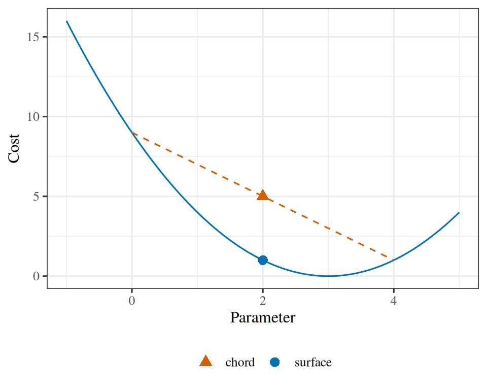
Example 6 Let \(J(\regcoef) = \regcoef^4 - 2\regcoef^2\). Its derivative is \(J'(\regcoef) = 4\regcoef^3 - 4\regcoef = 4\regcoef(\regcoef - 1)(\regcoef + 1)\), so the stationary points are \(\regcoef = -1\), \(0\) and \(1\).
- \(J(\pm 1) = -1\), and \(J(\regcoef) = \regcoef^2(\regcoef^2 - 2) > -1\) for every other \(\regcoef\) near \(\pm 1\), so both are local minima (local minimizers). They are in fact global minima.
- \(J(0) = 0\), and \(J(\regcoef) < 0\) for every nonzero \(\regcoef\) with \(\regcoef^2 < 2\), so \(\regcoef = 0\) is a local maximizer.
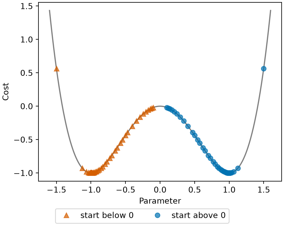
With a small step size, descent started at \(\regcoef_0 = 0.1\) runs away from \(0\) and settles at \(\regcoef = 1\), while a start at \(\regcoef_0 = -0.1\) settles at \(\regcoef = -1\). One equation, \(J' = 0\), produced three answers of two kinds.
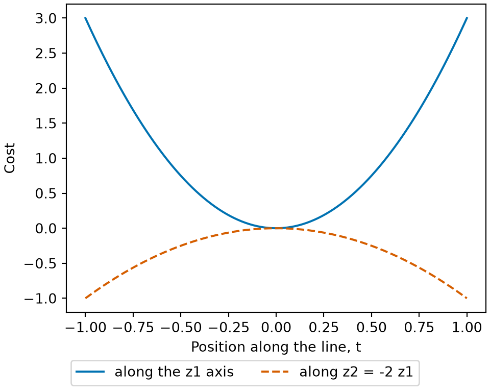
Example 7 The cost \(J(z_1, z_2) = 3z_1^2 + 4z_1 z_2 + z_2^2\) of Linear Regression has \(\grad J = (6z_1 + 4z_2,\ 4z_1 + 2z_2)\), which vanishes only at the origin. Along the \(z_1\) axis, \(J(t, 0) = 3t^2 > 0\). Along the line \(z_2 = -2z_1\),
\[ \begin{aligned} J(t, -2t) &= 3t^2 - 8t^2 + 4t^2 \\ &= -t^2 \\ &< 0. \end{aligned} \]
Every neighborhood of the origin holds points where \(J\) is larger and points where it is smaller, so the origin is neither a local minimum nor a local maximum. It is a saddle point.
A critical point where the surface flattens without turning around, such as \(\regcoef = 0\) for \(J(\regcoef) = \regcoef^3\), is a saddle point under this definition too, though it curves in only one direction.
Show code
library(ggplot2)
sp_cost <- function(z1, z2) 3 * z1^2 + 4 * z1 * z2 + z2^2
sp <- data.frame(t = seq(-1, 1, length.out = 201))
sp$axis <- sp_cost(sp$t, 0)
sp$line <- sp_cost(sp$t, -2 * sp$t)
sp_long <- data.frame(
  t = rep(sp$t, 2),
  cost = c(sp$axis, sp$line),
  path = rep(c("along the z1 axis", "along z2 = -2 z1"), each = nrow(sp))
)
ggplot(sp_long, aes(t, cost, colour = path, linetype = path)) +
  geom_line() +
  scale_colour_manual(values = c("#0072B2", "#D55E00")) +
  labs(x = "Position along the line, t", y = "Cost", colour = NULL, linetype = NULL)
Show code
import matplotlib.pyplot as plt
import numpy as np

def sp_cost(z1, z2):
    return 3 * z1 ** 2 + 4 * z1 * z2 + z2 ** 2

t_sp = np.linspace(-1, 1, 201)
fig, ax = plt.subplots(figsize=(5, 4), layout="constrained")
ax.plot(t_sp, sp_cost(t_sp, 0), color="#0072B2", linestyle="-", label="along the z1 axis");
ax.plot(t_sp, sp_cost(t_sp, -2 * t_sp), color="#D55E00", linestyle="--", label="along z2 = -2 z1");
ax.set_xlabel("Position along the line, t");
ax.set_ylabel("Cost");
fig.legend(loc="outside lower center", ncol=2);
plt.show()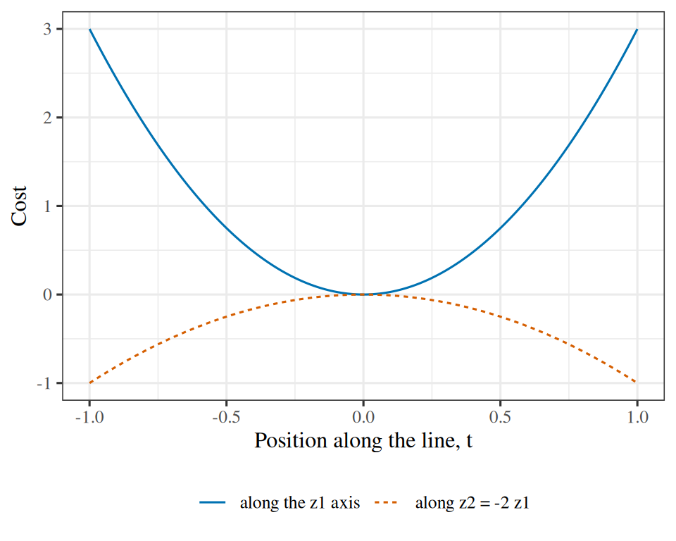
5 Non-convex costs
On a non-convex cost the answer is largely decided by \(\vcoef_0\), before a single step is taken. The next definition names the set of starting points that reach one minimum.
Definition 4 (Basin of attraction)
Definition 4 (Basin of attraction) The basin of attraction of a local minimum is the set of starting points \(\vcoef_0\) from which the descent iterates, for a given step size, converge to that minimum [8].
Example 8 Take \(J(\regcoef) = \regcoef^4 - 2\regcoef^2\) again, from Example 6. With a small step size, a start \(\regcoef_0 > 0\) of moderate size converges to the local minimum at \(\regcoef = 1\), and a start \(\regcoef_0 < 0\) of moderate size converges to the one at \(\regcoef = -1\). So the basin of attraction of \(\regcoef = 1\) is close to \((0, \infty)\), and that of \(\regcoef = -1\) is close to \((-\infty, 0)\). The single start \(\regcoef_0 = 0\) is the local maximum, where the gradient is zero and descent never moves. Which minimum the run reaches was settled by the sign of \(\regcoef_0\), before the first step.
The word “close” is needed because the basin depends on the step size. The curvature \(J''(\regcoef) = 12\regcoef^2 - 4\) grows without bound, so for any fixed step size a start far enough from the origin overshoots and diverges. The exact basin is a bounded stretch of each half-line, and it shrinks as the step size grows.
Show code
library(ggplot2)
bw_cost <- function(theta) theta^4 - 2 * theta^2
bw_step <- 0.05
bw_starts <- c(-1.5, -0.5, -0.1, 0.1, 0.5, 1.5)
bw_iterates <- do.call(rbind, lapply(bw_starts, function(start) {
  theta <- numeric(31)
  theta[1] <- start
  for (i in 2:31) theta[i] <- theta[i - 1] - bw_step * (4 * theta[i - 1]^3 - 4 * theta[i - 1])
  data.frame(start = start, theta = theta, basin = ifelse(start > 0, "start above 0", "start below 0"))
}))
bw_iterates$cost <- bw_cost(bw_iterates$theta)
ggplot(bw_iterates, aes(theta, cost)) +
  geom_function(fun = bw_cost, colour = "grey60", xlim = c(-1.6, 1.6)) +
  geom_point(aes(colour = basin, shape = basin), alpha = 0.7) +
  scale_colour_manual(values = c("start above 0" = "#0072B2", "start below 0" = "#D55E00")) +
  labs(x = "Parameter", y = "Cost", colour = NULL, shape = NULL)
Show code
import matplotlib.pyplot as plt
import numpy as np

def bw_cost(theta):
    return theta ** 4 - 2 * theta ** 2

bw_step = 0.05
fig, ax = plt.subplots(figsize=(5, 4), layout="constrained")
grid_bw = np.linspace(-1.6, 1.6, 321)
ax.plot(grid_bw, bw_cost(grid_bw), color="grey");
for start in [-1.5, -0.5, -0.1, 0.1, 0.5, 1.5]:
    theta = [start]
    for _ in range(30):
        theta.append(theta[-1] - bw_step * (4 * theta[-1] ** 3 - 4 * theta[-1]))
    theta = np.array(theta)
    above = start > 0
    ax.plot(theta, bw_cost(theta), linestyle="", alpha=0.7,
            color="#0072B2" if above else "#D55E00", marker="o" if above else "^",
            label=("start above 0" if above else "start below 0") if abs(start) == 0.1 else None);
ax.set_xlabel("Parameter");
ax.set_ylabel("Cost");
fig.legend(loc="outside lower center", ncol=2);
plt.show()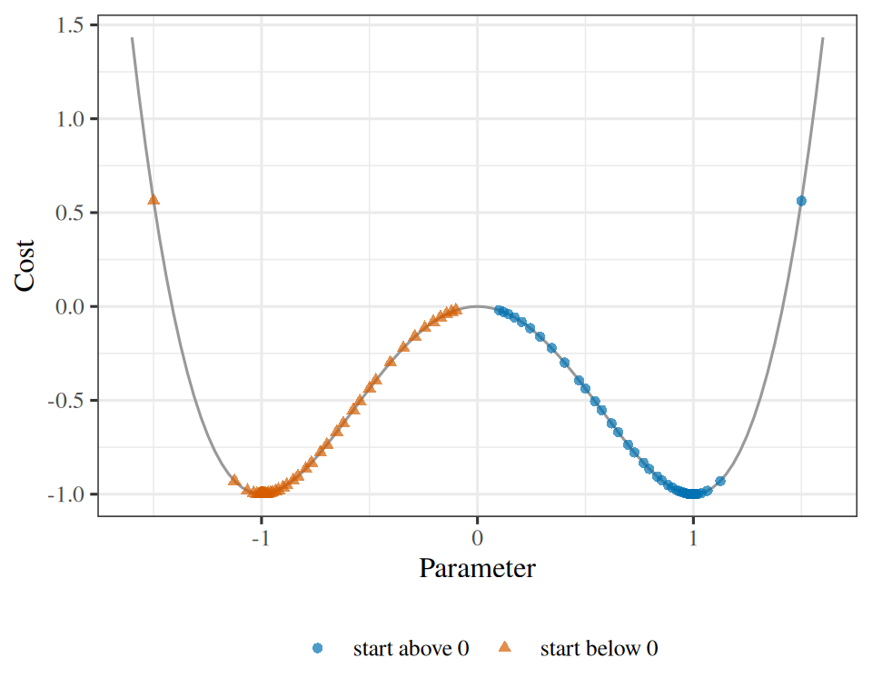
The basins of attraction (Definition 4) cover the parameter space, apart from a usually negligible set of starting points that reach no minimum. Level sets are the usual way to see them in two dimensions: the set of \(\vcoef\) where \(J\) takes a constant value, drawn for a few values of that constant. For the linear function of Linear Regression every level set is a hyperplane, and the picture carries little information. For a non-convex risk surface the level sets close into separate loops around separate minima, and counting the loops counts the basins.
Exercise 20 (Mark every zero-gradient point on a surface)
Exercise 20 (Mark every zero-gradient point on a surface) A risk surface over two coefficients is
\[ J(\vcoef) = \paren{\coef{1}^2 - 1}^2 + \paren{\coef{2}^2 - 1}^2. \]
Find every point where \(\grad J = \vzero\).
Solution 20. The cost is a sum of one term in each coefficient, so each partial derivative involves one coefficient:
\[ \derivf{J}{\coef{j}} = 4\coef{j}\paren{\coef{j}^2 - 1}, \qquad j = 1, 2. \]
Each is zero at \(\coef{j} \in \set{-1, 0, 1}\), and the gradient vanishes when both are. That gives \(3 \times 3 = 9\) points, the same three values as in Example 6, once in each coordinate. Figure 5 marks those nine points on the contours of \(J\).
Exercise 21 (Mark every zero-gradient point on a surface (part 2))
Exercise 21 (Mark every zero-gradient point on a surface (part 2)) Use the setup of Exercise 20.
Classify each point as a local minimizer, a local maximizer or a saddle point, using the sign of \(\derivf{^2 J}{\coef{1}^2}\) and of \(\derivf{^2 J}{\coef{2}^2}\). The mixed partial derivative is zero everywhere, so these two signs decide each case.
Solution 21. The second derivatives are \(\derivf{^2 J}{\coef{j}^2} = 12\coef{j}^2 - 4\). It is \(8 > 0\) where \(\coef{j} = \pm 1\) and \(-4 < 0\) where \(\coef{j} = 0\). So the surface curves up along an axis where that coordinate is \(\pm 1\) and down where it is \(0\):
- Both coordinates \(\pm 1\): curves up in both directions, a local minimum. There are four, \((\pm 1, \pm 1)\), each with \(J = 0\).
- Both coordinates \(0\): curves down in both directions, a local maximum. It is the origin, with \(J = 2\).
- One coordinate \(0\), the other \(\pm 1\): curves up in one direction and down in the other, a saddle point. There are four, \((0, \pm 1)\) and \((\pm 1, 0)\), each with \(J = 1\).
# Every combination of the three stationary values for each coordinate.
points <- expand.grid(b1 = c(-1, 0, 1), b2 = c(-1, 0, 1))

# The second derivative along each axis, from the formula above.
points$curve1 <- 12 * points$b1^2 - 4
points$curve2 <- 12 * points$b2^2 - 4
points$J <- (points$b1^2 - 1)^2 + (points$b2^2 - 1)^2

# Both curvatures positive: minimum. Both negative: maximum. Mixed: saddle.
points$type <- ifelse(
  points$curve1 > 0 & points$curve2 > 0, "minimum",
  ifelse(points$curve1 < 0 & points$curve2 < 0, "maximum", "saddle")
)
points
The table lists 4 minima, 1 maximum and 4 saddle points, matching the counts above.
Exercise 22 (Mark every zero-gradient point on a surface (part 3))
Exercise 22 (Mark every zero-gradient point on a surface (part 3)) Use the setup of Exercise 20.
Which of them can gradient descent settle at?
Solution 22. From almost every start, only at a local minimum, where every nearby point has a higher cost. Started exactly at the maximum the gradient is zero and descent never moves, and from every other start descent runs away from it. A saddle point attracts descent only from a thin set of starts. Along the line \(\coef{1} = 0\) the cost is \(1 + \paren{\coef{2}^2 - 1}^2\) in \(\coef{2}\) alone, so a start at \((0, 0.5)\) keeps \(\coef{1} = 0\) and moves to the saddle point \((0, 1)\). In the same way, a start on \(\coef{2} = 0\) with \(\coef{1} \ne 0\), such as \((0.5, 0)\), keeps \(\coef{2} = 0\) and converges to the saddle point \((\pm 1, 0)\). These lines have zero area, so a generic start, and any start with rounding error, leaves them and ends at a minimum (compare the single unstable start \(\regcoef_0 = 0\) in Example 8, where the maximum has only that one start). Because the minima here are four, which one a run reaches depends on the start.
Exercise 23 (Sketch the level sets)
Exercise 23 (Sketch the level sets) For the surface of Exercise 20, sketch the level sets \(\set{\vcoef : J(\vcoef) = c}\) for a value of \(c\) just above \(0\), for \(c = 1\), and for a large \(c\). Mark the nine zero-gradient points. How many separate curves does each level set have?
Solution 23. Near a local minimum the surface looks like a bowl, so its level sets there are small closed loops around the minimum. Near a saddle point the level set through the point is two curves that cross. The figure draws four values of \(c\) with the nine zero-gradient points marked.
Show code
library(ggplot2)

# The surface on a fine grid. The nine zero-gradient points, with their
# types, are the `points` table made in the previous solution.
grid <- expand.grid(
  b1 = seq(-2, 2, length.out = 300),
  b2 = seq(-2, 2, length.out = 300)
)
grid$J <- (grid$b1^2 - 1)^2 + (grid$b2^2 - 1)^2
points$type <- factor(points$type, levels = c("minimum", "maximum", "saddle"))

ggplot(grid) +
  aes(b1, b2) +
  geom_contour(aes(z = J, colour = after_stat(level)), breaks = c(0.25, 1, 1.5, 4)) +
  geom_point(aes(shape = type), data = points, size = 3) +
  scale_colour_viridis_c(name = "c", end = 0.85) +
  coord_fixed() +
  labs(
    x = expression("First coefficient, " * beta[1]),
    y = expression("Second coefficient, " * beta[2]),
    shape = NULL
  ) +
  theme(legend.position = "bottom")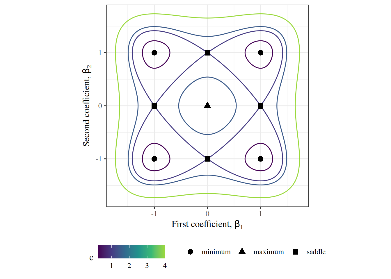
Show code
import matplotlib.pyplot as plt
import numpy as np

# The surface on a fine grid.
b = np.linspace(-2, 2, 300)
b1, b2 = np.meshgrid(b, b)
J = (b1**2 - 1) ** 2 + (b2**2 - 1) ** 2

fig, ax = plt.subplots(figsize=(5, 5))
cs = ax.contour(b1, b2, J, levels=[0.25, 1, 1.5, 4], cmap="viridis")
ax.clabel(cs, fmt="c = %g");
# Minima at (+-1, +-1), the maximum at the origin, saddles on the axes.
ax.scatter([-1, -1, 1, 1], [-1, 1, -1, 1], marker="o", c="k", label="minimum");
ax.scatter([0], [0], marker="^", c="k", label="maximum");
ax.scatter([0, 0, -1, 1], [-1, 1, 0, 0], marker="s", c="k", label="saddle");
ax.set_aspect("equal");
ax.set_xlabel(r"First coefficient, $\beta_1$");
ax.set_ylabel(r"Second coefficient, $\beta_2$");
ax.legend(loc="upper center", bbox_to_anchor=(0.5, -0.15), ncol=3);
fig.tight_layout()  # make room for the legend below the axes
plt.show()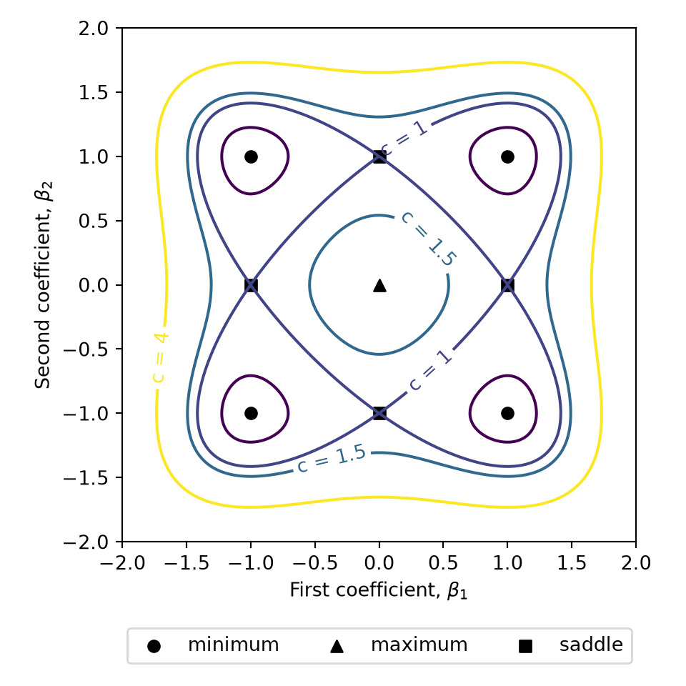
For \(c\) just above \(0\) the level set is four small loops, one around each minimum. At \(c = 1\) the four loops have grown until neighbouring ones touch, and they meet exactly at the four saddle points, so the level set is a single curve that crosses itself at each saddle. For \(c = 1.5\), between the saddles’ value \(1\) and the maximum’s value \(2\), the loops have merged into an outer curve around all four minima and a small inner loop around the maximum. For a large \(c\) only the outer curve remains, and it is a single closed curve. Counting the loops at a small \(c\) counts the basins of attraction (Definition 4), and the saddles are where the basins touch.
5.1 Weight-space symmetry
A neural network’s surface has a specific and easily described source of multiplicity. Take a hidden layer of \(L\) units and permute them — relabel unit 1 as unit 3 and so on — carrying each unit’s incoming weights and its outgoing weights along with it. Every unit still receives the same inputs and still contributes the same quantity to the layer above, so the function the network computes does not change. There are \(L!\) such relabelings, and a network with \(K\) hidden layers of \(L\) units each admits them independently in every layer, giving \((L!)^{K}\) weight vectors that compute one and the same function [9, Sec. 5.1.1].
If the hidden non-linearity is odd, as \(\tanh\) is, a second family joins them. Negate every weight and the bias feeding one unit and that unit’s output flips sign, because \(\tanh(-a) = -\tanh(a)\); negate its outgoing weights as well and the flip cancels downstream. That is a further factor of \(2^L\) per layer, so a \(\tanh\) layer carries \(L!\,2^L\) symmetries rather than \(L!\).
The consequence for optimization is that “this objective has an enormous number of local minima” overstates the difficulty. If one configuration is a local minimum then so is every one of its relabelings, and they are one solution written down in different orders. A surface with many equivalent copies of a minimum is no harder to descend than a surface carrying one copy.
5.2 Which obstacles actually matter
The original worry about non-convexity was local minima: with no convexity guarantee, nothing promises that the point found is the best one. That worry has largely not been confirmed in practice. The local minima that large networks actually reach tend to have training losses close to one another, and a local minimum bad enough to matter is hard to exhibit.
Saddle points and flat regions turned out to be the harder problem. A stationary point is a minimum only if the surface curves upward along every direction, and as the number of parameters grows that becomes an increasingly unlikely condition, so stationary points at a given height above the minimum are overwhelmingly saddles rather than minima [10]. Exactly at a saddle the gradient is zero and descent halts. A little to one side of it a descent direction exists, and the iterates eventually find it, so a saddle usually slows the run rather than ending it.
Definition 5 (Plateau)
Definition 5 (Plateau) A plateau is a region where \(\norm{\grad J}\) is small but nonzero, so the surface is nearly flat without containing a stationary point.
Example 9 Take the one-parameter logistic cost \(J(\regcoef) = \log\paren{1 + e^{-\regcoef}}\), the loss of a single training point that the model should score as positive. Its derivative is \(J'(\regcoef) = -1/(1 + e^{\regcoef})\), which is negative for every \(\regcoef\), so \(J\) has no stationary point at all.
At \(\regcoef = 0\) the gradient has size \(|J'(0)| = 0.5\). At \(\regcoef = 10\) it has size \(4.54\times 10^{-5}\), which is small but not zero. A descent step is the gradient times the step size, so the iterates keep moving to the right, more and more slowly. Everything to the right of about \(\regcoef = 10\) is a plateau (Definition 5), and a run that enters it has not converged; it has only slowed down.
Show code
library(ggplot2)
pl_grad <- function(beta) 1 / (1 + exp(beta))
pl_marks <- data.frame(beta = c(0, 10))
pl_marks$size <- pl_grad(pl_marks$beta)
ggplot(data.frame(beta = c(-5, 15)), aes(beta)) +
  geom_function(fun = pl_grad, colour = "#0072B2") +
  geom_point(data = pl_marks, aes(beta, size), colour = "#D55E00", shape = 17, size = 3) +
  scale_y_log10() +
  labs(x = "Parameter", y = "Size of the gradient (log scale)")
Show code
import matplotlib.pyplot as plt
import numpy as np

def pl_grad(beta):
    return 1 / (1 + np.exp(beta))

grid_pl = np.linspace(-5, 15, 401)
marks_pl = np.array([0, 10])
fig, ax = plt.subplots(figsize=(5, 4), layout="constrained")
ax.plot(grid_pl, pl_grad(grid_pl), color="#0072B2");
ax.plot(marks_pl, pl_grad(marks_pl), color="#D55E00", marker="^", markersize=8, linestyle="");
ax.set_yscale("log");
ax.set_xlabel("Parameter");
ax.set_ylabel("Size of the gradient (log scale)");
plt.show()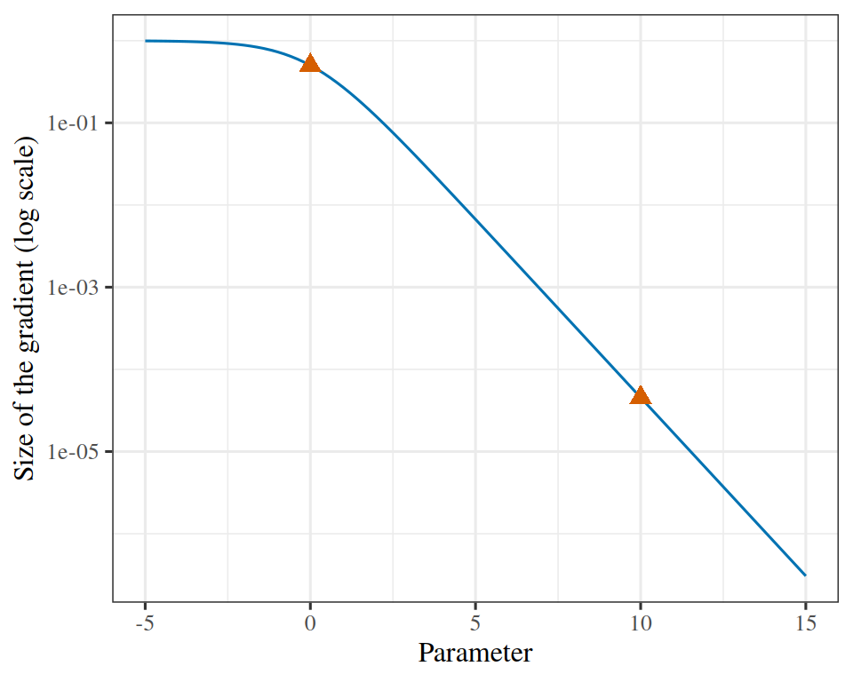
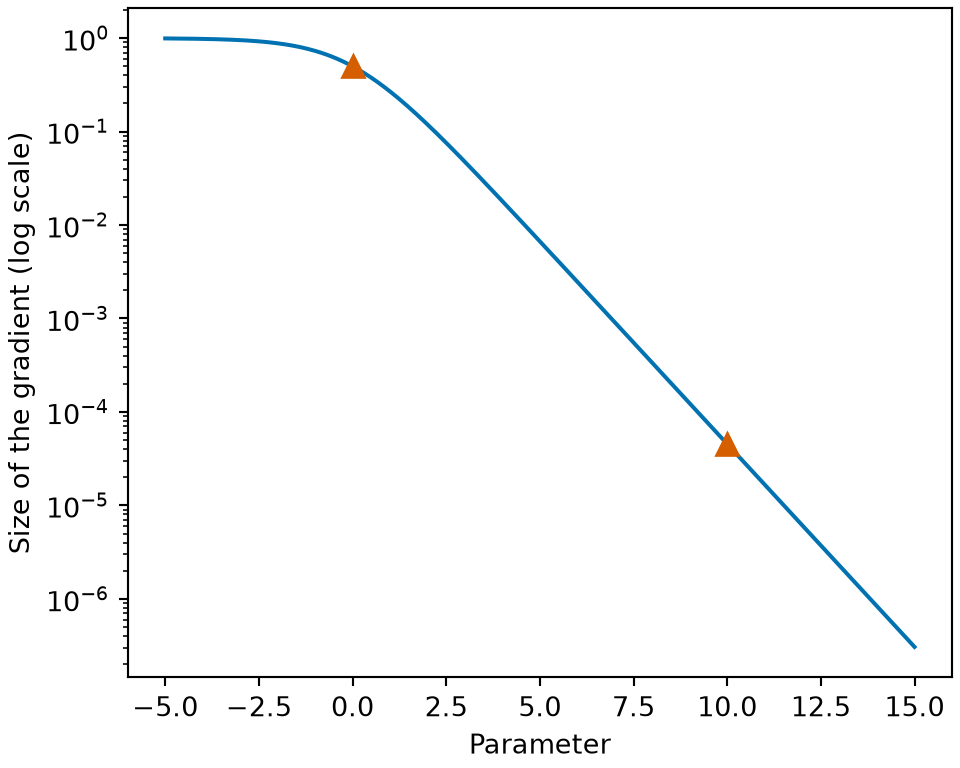
On a plateau the gradient is small, so the steps are small, and progress can stall for a long stretch with nothing having gone wrong, in the sense of the algorithm being stuck. Saturated units are the usual cause: a unit sitting in the flat part of its non-linearity has a derivative near zero, so every weight feeding it receives almost no gradient. Backpropagation covers the extreme case, a unit whose derivative is exactly zero and stays there, and the two failures that depth adds on top of this one: vanishing and exploding gradients.
Watch
Hutchinson covers critical points, saddle points and other optimization challenges (24 min) [5]. The video site requires a login, which enrolled students find in the syllabus.
6 Where to start
For a convex cost the starting point does not change the answer. Every run reaches the same minimum, so \(\vcoef_0\) decides only how long the run takes.
\(\vcoef_0 = \vzero\) is the usual choice, and it is not arbitrary. It is the null model: for logistic regression it predicts probability \(1/2\) for every observation, so the run begins from no claim at all and every subsequent step is evidence the data supplied. It is also the centre of an \(L_2\) penalty, so a run stopped early has been shrunk toward the same point the penalty shrinks toward. That is why early stopping acts as a regularizer.
For a cost that is not convex the starting point decides which minimum you reach, and there is no longer one right answer to reach. Two things follow.
Starting at \(\vcoef_0 = \vzero\) becomes actively wrong for a neural network: every unit in a layer then computes the same function and receives the same gradient, so they stay identical forever and the layer has the capacity of a single unit. The weights have to be initialized randomly, to break that symmetry.
And the scale of that randomness matters separately. Draw the weights too large and the activations saturate, in exactly the sense of the flat regions this chapter keeps meeting; draw them too small and the signal shrinks toward zero through the layers. The standard schemes set the variance from the number of units feeding each layer, and the chapter on neural networks takes that up.
7 Choosing the step size
With a constant \(\learnrate\) there are two ways to go wrong, and the Week 6 notes name both:
Too big: the iterates overshoot and \(\norm{\vcoef_t} \to \infty\).
Too small: every step is downhill, but there are far too many of them.
Figure 7 draws both failures, and a step size between them, on one elongated cost. Exercise 10 has already shown both ends of that range on real numbers. For least squares the boundary between them can be located exactly, because the cost is a quadratic and the whole trajectory can be written in closed form.
Read
GeeksforGeeks explains the learning rate [11].
Show code
# HTML formats get an interactive plotly figure;
# the handout and other formats get the same level sets and paths
# drawn with ggplot2.
# The cost is J(w) = (a * w1^2 + b * w2^2) / 2,
# so its gradient is (a * w1, b * w2),
# and one step multiplies the coordinates by 1 - h * a and 1 - h * b.
# Step sizes are multiples of 1 / b, the largest curvature.
curv <- c(a = 1, b = 10)
start <- c(-3, 1)
step_multiples <- c(small = 0.1, near = 1, large = 2.1)
n_steps <- 25

descend <- function(h) {
  path <- matrix(NA_real_, nrow = n_steps + 1, ncol = 2)
  path[1, ] <- start
  for (t in seq_len(n_steps)) {
    path[t + 1, ] <- path[t, ] - h * curv * path[t, ]
  }
  path
}
paths <- lapply(step_multiples / curv[["b"]], descend)

# The plotted window.
# Every point is drawn,
# so the plot clips a diverging path at the edge,
# where it visibly leaves the picture.
xlim <- c(-3.5, 3.5)
ylim <- c(-1.5, 1.5)
grid_x <- seq(xlim[1], xlim[2], length.out = 120)
grid_y <- seq(ylim[1], ylim[2], length.out = 120)
cost <- outer(grid_x, grid_y, function(w1, w2) {
  (curv[["a"]] * w1^2 + curv[["b"]] * w2^2) / 2
})
labels <- c(
  small = "small step: 0.1 / largest curvature",
  near = "middle step: 1 / largest curvature",
  large = "large step: 2.1 / largest curvature"
)
colors <- c(small = "#1f77b4", near = "#2ca02c", large = "#d95f02")

if (knitr::is_html_output()) {
  library(plotly)

  widget <- plot_ly() |>
    add_contour(
      x = grid_x,
      y = grid_y,
      z = t(cost),
      showscale = FALSE,
      colorscale = list(c(0, "#f2f2f2"), c(1, "#cccccc")),
      contours = list(coloring = "none", showlabels = FALSE),
      line = list(color = "#888888", width = 1),
      hoverinfo = "skip",
      name = "level sets",
      showlegend = FALSE
    )
  for (nm in names(paths)) {
    widget <- widget |>
      add_trace(
        x = paths[[nm]][, 1],
        y = paths[[nm]][, 2],
        type = "scatter",
        mode = "lines+markers",
        name = labels[[nm]],
        line = list(color = colors[[nm]]),
        marker = list(color = colors[[nm]]),
        hovertemplate = "first %{x:.2f}<br>second %{y:.2f}<extra></extra>"
      )
  }
  widget <- widget |>
    layout(
      xaxis = list(
        title = "first coefficient",
        range = xlim,
        zeroline = FALSE,
        constrain = "domain"
      ),
      yaxis = list(
        title = "second coefficient",
        range = ylim,
        zeroline = FALSE,
        scaleanchor = "x",
        scaleratio = 1,
        constrain = "domain"
      ),
      legend = list(orientation = "h", x = 0.5, xanchor = "center", y = -0.2),
      margin = list(t = 10, b = 90)
    ) |>
    config(displaylogo = FALSE, responsive = TRUE)

  # The alt text: a plotly widget has none of its own.
  htmltools::div(
    role = "img",
    `aria-label` = paste(
      "Interactive contour plot of an elongated quadratic cost",
      "with three gradient-descent paths from one starting point:",
      "a small step that crawls along the valley,",
      "a step of one over the largest curvature",
      "that drops onto the valley floor at once",
      "and then follows it toward the minimum,",
      "and a larger step that overshoots back and forth across the valley",
      "and leaves the plot."
    ),
    widget
  )
} else {
  library(ggplot2)

  level_sets <- expand.grid(first = grid_x, second = grid_y)
  level_sets$cost <- as.vector(cost)
  path_points <- do.call(
    rbind,
    lapply(names(paths), function(nm) {
      data.frame(
        first = paths[[nm]][, 1],
        second = paths[[nm]][, 2],
        step = labels[[nm]]
      )
    })
  )
  path_points$step <- factor(path_points$step, levels = unname(labels))

  ggplot() +
    geom_contour(
      data = level_sets,
      mapping = aes(x = first, y = second, z = cost),
      colour = "grey60",
      linewidth = 0.3
    ) +
    geom_path(
      data = path_points,
      mapping = aes(x = first, y = second, colour = step)
    ) +
    geom_point(
      data = path_points,
      mapping = aes(x = first, y = second, colour = step),
      size = 1
    ) +
    scale_colour_manual(values = setNames(unname(colors), unname(labels))) +
    coord_fixed(xlim = xlim, ylim = ylim, expand = FALSE) +
    labs(
      x = "first coefficient",
      y = "second coefficient",
      colour = NULL
    ) +
    theme(
      legend.position = "bottom"
    )
}Exercise 24 (Rewrite the cost around its minimum)
Exercise 24 (Rewrite the cost around its minimum) Before we can say which step sizes work, we need to know what gradient descent does to the error \(\ve_t = \vcoef_t - \vcoef^\star\) rather than to the cost. For least squares this can be worked out exactly, because the cost is a quadratic.
Let \(\vcoef^\star\) solve the normal equations. Show that
\[J(\vcoef) = (\vcoef - \vcoef^\star)^\top \stprod{\design} (\vcoef - \vcoef^\star) + J(\vcoef^\star)\]
by writing \(\design\vcoef - \vy = \design(\vcoef - \vcoef^\star) + (\design\vcoef^\star - \vy)\) and expanding.
Solution 24. Write \(\vr^\star = \design\vcoef^\star - \vy\) for the residual at the minimum, and \(\ve = \vcoef - \vcoef^\star\). Then \(\design\vcoef - \vy = \design\ve + \vr^\star\) and
\[ \begin{aligned} J(\vcoef) &= \norm{\design\ve + \vr^\star}_2^2 \\ &= \ve^\top \stprod{\design} \ve + 2\,\ve^\top \tp{\design} \vr^\star +\norm{\vr^\star}_2^2 \end{aligned} \]
The cross term vanishes. Solve the normal equations by hand showed \(\tp{\design} \vr^\star = \vzero\) — the residual at the optimum is orthogonal to every column of \(\design\) — so the middle term is \(2\ve^\top \vzero = 0\), leaving
\[J(\vcoef) = \ve^\top \stprod{\design} \ve + J(\vcoef^\star)\]
Exercise 25 (Rewrite the cost around its minimum (part 2))
Exercise 25 (Rewrite the cost around its minimum (part 2)) Use the setup of Exercise 24.
Read off what the level sets of \(J\) look like, and what fixes their shape.
Solution 25. \(J\) is a constant plus a quadratic form in \(\ve\), so its level sets are ellipsoids centred on \(\vcoef^\star\). Their shape and orientation come entirely from \(\stprod{\design}\): the axes point along its eigenvectors, and an axis is long where the eigenvalue is small and short where it is large. The data determines the shape of the cost surface; \(\vy\) only determines where its centre is and what its minimum value is.
For our three points, \(\stprod{\design} = \sbmat{ 3 & 3 \\ 3 & 5 }\), whose eigenvalues are \(4 \pm \sqrt{10}\), so \(\eigval_{\max} \approx 7.162\) and \(\eigval_{\min} \approx 0.838\). A level set of \(\ve^\top \stprod{\design} \ve\) has semi-axis length proportional to \(1/\sqrt{\eigval}\), so it is the square root of the eigenvalue ratio that sets the shape: the contours are ellipses about \(\sqrt{8.55} = 2.92\) times longer one way than the other. The long axis runs along the \(\eigval_{\min}\) eigenvector, about \(36^\circ\) below the intercept axis, and the short axis along the \(\eigval_{\max}\) eigenvector at right angles to it.
Exercise 26 (Rewrite the cost around its minimum (part 3))
Exercise 26 (Rewrite the cost around its minimum (part 3)) Use the setup of Exercise 24.
Use the identity to write \(\grad J\) in terms of \(\ve = \vcoef - \vcoef^\star\), and then show that one gradient-descent step gives
\[\ve_{t+1} = (I - 2\learnrate \stprod{\design})\,\ve_t\]
Solution 26. Differentiating the identity, the constant drops out and
\[\grad J(\vcoef) = 2\stprod{\design}\,\ve\]
which is worth checking against the original form:
\[ \begin{aligned} 2\tp{\design}(\design\vcoef - \vy) &= 2\tp{\design}(\design\ve + \vr^\star) \\ &= 2\stprod{\design} \ve, \end{aligned} \]
the same thing. Now subtract \(\vcoef^\star\) from both sides of the update:
\[\vcoef_{t+1} - \vcoef^\star = \vcoef_t - \vcoef^\star - \learnrate\grad J(\vcoef_t) = \ve_t - 2\learnrate \stprod{\design}\,\ve_t = (I - 2\learnrate \stprod{\design})\,\ve_t\]
Exercise 27 (Rewrite the cost around its minimum (part 4))
Exercise 27 (Rewrite the cost around its minimum (part 4)) Use the setup of Exercise 24.
Explain why this one line, and no further algebra, already tells you that gradient descent on a quadratic either converges geometrically or diverges geometrically, with the boundary case in between held at constant size.
Solution 27. Because the recursion is linear and its matrix does not change from step to step. Iterating it gives \(\ve_t = (I - 2\learnrate \stprod{\design})^t\,\ve_0\), so the error is a fixed matrix raised to the power \(t\). A matrix power either shrinks every component geometrically or blows one up geometrically, depending on that matrix’s eigenvalues, and the cost follows the error by Solution 24: \(J(\vcoef_t) - J(\vcoef^\star)\) is a quadratic form in \(\ve_t\), so it shrinks or grows like the square of whatever the error does.
There is no third behaviour to worry about, and no need to argue about it case by case. Exercise 29 turns this into a rule for \(\learnrate\).
Exercise 28 (Find the exact range of step sizes that converge)
Exercise 28 (Find the exact range of step sizes that converge) Exercise 24 gave \(\ve_{t+1} = (I - 2\learnrate\stprod{\design})\ve_t\). Turn that into a condition on \(\learnrate\).
Let \(\stprod{\design} = Q\Eigvals \tp{Q}\) be its eigendecomposition, with eigenvalues \(\eigval_1, \ldots, \eigval_{\ninputvars+1} \ge 0\). Write \(\ve_t\) in the eigenvector basis and show that each coordinate evolves on its own, multiplied each step by a scalar you should name.
Solution 28. Since \(Q\) is orthogonal, \(I - 2\learnrate\stprod{\design} = Q(I - 2\learnrate\Eigvals)\tp{Q}\). Let \(\vz_t = \tp{Q} \ve_t\) hold the error’s coordinates in the eigenvector basis. Then
\[\vz_{t+1} = (I - 2\learnrate\Eigvals)\,\vz_t, \qquad\text{so}\qquad z_{t+1,j} = (1 - 2\learnrate\eigval_j)\,z_{t,j}\]
\(I - 2\learnrate\Eigvals\) is diagonal, so the coordinates do not mix: each one is its own one-dimensional problem, multiplied every step by
\[\coordfactor_j = 1 - 2\learnrate\eigval_j\]
Gradient descent on a quadratic is \(\ninputvars+1\) independent geometric sequences written as a matrix.
Exercise 29 (Find the exact range of step sizes that converge (part 2))
Exercise 29 (Find the exact range of step sizes that converge (part 2)) Use the setup of Exercise 28.
State the condition on \(\learnrate\) under which every coordinate shrinks, and simplify it to a single upper bound.
Solution 29. Coordinate \(j\) shrinks exactly when \(|\coordfactor_j| < 1\), that is
\[-1 < 1 - 2\learnrate\eigval_j < 1 \quad\Longleftrightarrow\quad 0 < \learnrate < \frac{1}{\eigval_j}\]
using \(\eigval_j > 0\) for the division. Every coordinate shrinks when this holds for all \(j\), and the binding case is the largest eigenvalue:
\[0 < \learnrate < \frac{1}{\eigval_{\max}}\]
The smallest eigenvalue plays no part in whether we converge. It decides how slowly, which is Exercise 33. (If some \(\eigval_j = 0\) then \(\coordfactor_j = 1\) and that coordinate never moves — the direction \(\design\) cannot see; see When \(\stprod{\design}\) is not invertible. Gradient descent leaves it at its initial value, which is one way of choosing among the infinitely many solutions.)
Exercise 30 (Find the exact range of step sizes that converge (part 3))
Exercise 30 (Find the exact range of step sizes that converge (part 3)) Use the setup of Exercise 28.
Evaluate that bound for our three-point \(\design\), where \(\eigval_{\max} = 4 + \sqrt{10}\).
Solution 30. \[ \begin{aligned} \frac{1}{\eigval_{\max}} &= \frac{1}{4 + \sqrt{10}} \\ &= \frac{4 - \sqrt{10}}{16 - 10} \\ &= \frac{4 - \sqrt{10}}{6} \\ &\approx 0.1396 \end{aligned} \]
Exercise 31 (Find the exact range of step sizes that converge (part 4))
Exercise 31 (Find the exact range of step sizes that converge (part 4)) Use the setup of Exercise 28.
Compute the two multipliers for each of \(\learnrate = \tfrac{1}{20}\), \(\learnrate = \tfrac{1}{10}\), \(\learnrate = \tfrac{3}{20}\), and check the answers against what Exercise 10 actually observed.
Solution 31. With \(\eigval_{\min} = 4 - \sqrt{10} \approx 0.8377\) and \(\eigval_{\max} = 4 + \sqrt{10} \approx 7.1623\):
| \(\learnrate\) | \(\coordfactor_{\min} = 1 - 2\learnrate\eigval_{\min}\) | \(\coordfactor_{\max} = 1 - 2\learnrate\eigval_{\max}\) | \(\max_j\abs{\coordfactor_j}\) | verdict |
|---|---|---|---|---|
| \(1/20 = 0.05\) | \(0.9162\) | \(0.2838\) | \(0.9162\) | converges |
| \(1/10 = 0.10\) | \(0.8325\) | \(-0.4325\) | \(0.8325\) | converges |
| \(3/20 = 0.15\) | \(0.7487\) | \(-1.1487\) | \(1.1487\) | diverges |
This matches Exercise 10: the first two steps lowered the cost and the third raised it, and \(0.15\) is the only one of the three above the bound \(0.1396\) from Solution 30.
It also says something Exercise 10 could not. Judged after one step, \(\learnrate = 1/20\) looked best — it reached \(J = 2.3\) where \(\learnrate = 1/10\) reached only \(4.2\). Judged over many steps, \(\learnrate = 1/10\) is the better choice, because its worst multiplier is \(0.8325\) against \(0.9162\). One step is not evidence about a step size.
Exercise 32 (Find the exact range of step sizes that converge (part 5))
Exercise 32 (Find the exact range of step sizes that converge (part 5)) Use the setup of Exercise 28.
At \(\learnrate = 1/10\) one multiplier is negative. Say what that looks like if you plot the path, and whether it is a problem.
Solution 32. A negative multiplier means that coordinate of the error changes sign every step while shrinking in size, so the path zig-zags across the valley floor rather than sliding along it, crossing \(\vcoef^\star\) in that direction on every step.
It is not a problem as long as \(|\coordfactor| < 1\). A step slightly too long for the steepest direction zig-zags like this while it is still short enough to converge, and here the zig-zag gives a better rate in the slow direction. It becomes a problem only at \(|\coordfactor| \ge 1\), where the zig-zag grows instead of shrinking — which is the \(\learnrate = 3/20\) row, and is exactly the picture of that step climbing the far wall in Exercise 10.
Exercise 33 (Find the best constant step size, and what limits it)
Exercise 33 (Find the best constant step size, and what limits it) Exercise 28 says which \(\learnrate\) converge. This one asks which converges fastest, and what limits that speed.
The error shrinks each step by at worst \(\convrate(\learnrate) = \max_j |1 - 2\learnrate\eigval_j|\), so the best constant step size is the one minimizing \(\convrate\).
Only the largest and smallest eigenvalues can attain the maximum. Sketch \(|1 - 2\learnrate\eigval_{\min}|\) and \(|1 - 2\learnrate\eigval_{\max}|\) as functions of \(\learnrate\) and argue that the best \(\learnrate\) is where the two curves cross.
Solution 33. Each \(|1 - 2\learnrate\eigval_j|\) is a V shape: it falls from \(1\) at \(\learnrate=0\), reaches zero at \(\learnrate = 1/(2\lambda_j)\), and rises again. The V for \(\lambda_{\max}\) turns first and climbs steeply; the V for \(\eigval_{\min}\) is still falling gently. Every other eigenvalue sits between them, so the maximum of the whole family is the upper envelope of just these two.
For small \(\learnrate\) that envelope is the still-falling \(|1 - 2\learnrate\eigval_{\min}|\); for large \(\learnrate\) it is the rising \(|1 - 2\learnrate\eigval_{\max}|\). One is decreasing and the other increasing, so their maximum is minimized exactly where they meet.
Exercise 34 (Find the best constant step size, and what limits it (part 2))
Exercise 34 (Find the best constant step size, and what limits it (part 2)) Use the setup of Exercise 33.
Solve for that \(\learnrate\), and show that the resulting rate is
\[\convrate^\star = \frac{\condnum - 1}{\condnum + 1}, \qquad \condnum = \frac{\eigval_{\max}}{\eigval_{\min}}\]
the condition number of \(\stprod{\design}\).
Solution 34. At the crossing the \(\eigval_{\max}\) branch is already past its turn, so \(1 - 2\learnrate\eigval_{\max}\) is negative and the equation is
\[1 - 2\learnrate\eigval_{\min} = -(1 - 2\learnrate\eigval_{\max}) \quad\Longrightarrow\quad 2 = 2\learnrate(\eigval_{\min} + \eigval_{\max}) \quad\Longrightarrow\quad \learnrate^\star = \frac{1}{\eigval_{\min} + \eigval_{\max}}\]
Substituting back,
\[ \begin{aligned} \convrate^\star &= 1 - \frac{2\eigval_{\min}}{\eigval_{\min} + \eigval_{\max}} \\ &= \frac{\eigval_{\max} - \eigval_{\min}}{\eigval_{\max} + \eigval_{\min}} \\ &= \frac{\condnum - 1}{\condnum + 1} \end{aligned} \]
dividing through by \(\eigval_{\min}\) in the last step. Note \(\learnrate^\star < 1/\eigval_{\max}\), so the best constant step is well inside the range Exercise 29 allows; the bound is not tight.
Exercise 35 (Find the best constant step size, and what limits it (part 3))
Exercise 35 (Find the best constant step size, and what limits it (part 3)) Use the setup of Exercise 33.
Evaluate \(\learnrate^\star\), \(\condnum\) and \(\convrate^\star\) for our three-point \(\design\). You may use \(\eigval_{\min} + \eigval_{\max} = \tr(\stprod{\design})\) to save arithmetic.
Solution 35. \(\tr(\stprod{\design}) = 3 + 5 = 8\), so \(\eigval_{\min} + \eigval_{\max} = 8\) and
\[ \begin{aligned} \learnrate^\star &= \tfrac{1}{8} \\ &= 0.125 \end{aligned} \]
with
\[ \begin{aligned} \condnum &= \frac{4 + \sqrt{10}}{4 - \sqrt{10}} \\ &= \frac{(4+\sqrt{10})^2}{6} \\ &= \frac{26 + 8\sqrt{10}}{6} \\ &= \frac{13 + 4\sqrt{10}}{3} \\ &\approx 8.5497 \end{aligned} \]
\[\convrate^\star = \frac{\condnum - 1}{\condnum + 1} \approx 0.7906\]
Exercise 36 (Find the best constant step size, and what limits it (part 4))
Exercise 36 (Find the best constant step size, and what limits it (part 4)) Use the setup of Exercise 33.
How many steps does it take to cut the error by a factor of ten, at \(\learnrate^\star\) and at each of \(\learnrate = 1/20\) and \(\learnrate = 1/10\)?
Solution 36. Cutting the error by ten needs \(\convrate^{\,t} \le 0.1\), so \(t \ge \log(0.1)/\log\convrate\).
| \(\learnrate\) | \(\convrate\) | steps per factor of ten |
|---|---|---|
| \(1/8 = 0.125\) | \(0.7906\) | \(9.80 \to 10\) |
| \(1/10 = 0.1\) | \(0.8325\) | \(12.56 \to 13\) |
| \(1/20 = 0.05\) | \(0.9162\) | \(26.32 \to 27\) |
Halving the step from \(1/10\) to \(1/20\) roughly doubles the work, which is the “too small takes a long time” half of the constant-step warning made precise.
Exercise 37 (Find the best constant step size, and what limits it (part 5))
Exercise 37 (Find the best constant step size, and what limits it (part 5)) Use the setup of Exercise 33.
What happens to \(\convrate^\star\) as \(\condnum \to \infty\)?
Solution 37. As \(\condnum \to \infty\), \(\convrate^\star \to 1\): the rate approaches no progress at all, and the number of steps per digit of accuracy grows without bound. Gradient descent slows down in proportion to how badly conditioned the problem is, and no choice of constant step rescues it, because \(\convrate^\star\) is already the best available.
Exercise 38 (Find the best constant step size, and what limits it (part 6))
Exercise 38 (Find the best constant step size, and what limits it (part 6)) Use the setup of Exercise 33.
What does a large \(\condnum\) say about the data?
Solution 38. A large \(\condnum\) says the columns of \(\design\) are close to collinear — there is a direction in feature space the data barely varies along, so the cost is nearly flat there and the contours are a long narrow valley. Descent alternates between the valley sides and advances slowly along its bottom.
Exercise 39 (Find the best constant step size, and what limits it (part 7))
Exercise 39 (Find the best constant step size, and what limits it (part 7)) Use the setup of Exercise 33.
Name one thing you could change to make \(\condnum\) smaller without changing the model.
Solution 39. The least expensive fix that leaves the model alone is to rescale the features, usually by centring each one and dividing by its standard deviation. A feature measured in millimetres and one measured in kilometres have columns a factor of \(10^{6}\) apart, and \(\stprod{\design}\) is quadratic in the column scale, so their eigenvalues come out about \(10^{12}\) apart for reasons that have nothing to do with the data. Standardizing removes that entirely. The fitted function is unchanged — the coefficients simply absorb the scaling — but \(\condnum\) can fall by orders of magnitude, so the same algorithm converges in a fraction of the steps.
This is also the actual reason ridge regression often trains faster: adding \(\regpar I\) to \(\stprod{\design}\) raises every eigenvalue by \(\regpar\), which lifts \(\regpar_{\min}\) proportionally far more than \(\regpar_{\max}\) and so shrinks \(\condnum\). That is a change to the model, though, not just to the arithmetic.
Theorem 1 (The best constant step size)
Theorem 1 (The best constant step size) For gradient descent on the least squares cost with \(\convrate(h) = \max_j |1 - 2h\eigval_j|\), where \(\eigval_1, \dots, \eigval_p\) are the eigenvalues of \(\stprod{\design}\), the rate is smallest at
\[h^\star = \frac{1}{\eigval_{\min} + \eigval_{\max}},\]
and then
\[\convrate^\star = \frac{\condnum - 1}{\condnum + 1}, \qquad \condnum = \frac{\eigval_{\max}}{\eigval_{\min}}.\]
Proof
Proof. By Solution 33 and Solution 34.
Example 10 (A line fit on four points)
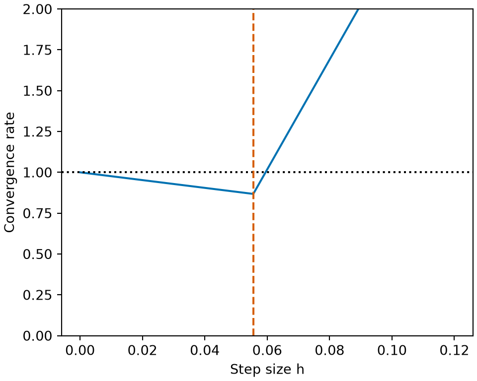
Example 10 (A line fit on four points) Take the design matrix with a column of ones and the inputs \(0, 1, 2, 3\). Compute \(h^\star\) and \(\convrate^\star\) from Theorem 1, and check them against a direct search over \(h\):
import numpy as np

X_ls = np.column_stack([np.ones(4), np.arange(4.0)])
ev = np.linalg.eigvalsh(X_ls.T @ X_ls)
h_star = 1 / (ev.min() + ev.max())
kappa = ev.max() / ev.min()
rho = lambda h: np.max(np.abs(1 - 2 * h * ev))
grid = np.linspace(1e-4, 0.2, 20001)
print(h_star, grid[np.argmin([rho(h) for h in grid])])
0.05555555555555555 0.055552260000000010.8678055195451838 0.8678055195451838[1] 0.05555556 0.05555226[1] 0.8678055 0.8678055The search finds the same step size, and the rate matches the formula.
Show code
library(ggplot2)
oc <- data.frame(h = seq(1e-4, 0.12, length.out = 400))
oc$rate <- sapply(oc$h, rho)
ggplot(oc, aes(h, rate)) +
  geom_line(colour = "#0072B2") +
  geom_hline(yintercept = 1, linetype = "dotted") +
  geom_vline(xintercept = h_star, colour = "#D55E00", linetype = "dashed") +
  coord_cartesian(ylim = c(0, 2)) +
  labs(x = "Step size h", y = "Convergence rate")
Show code
import matplotlib.pyplot as plt
import numpy as np

h_oc = np.linspace(1e-4, 0.12, 400)
fig, ax = plt.subplots(figsize=(5, 4), layout="constrained")
ax.plot(h_oc, [rho(h) for h in h_oc], color="#0072B2");
ax.axhline(1, color="black", linestyle=":");
ax.axvline(h_star, color="#D55E00", linestyle="--");
ax.set_ylim(0, 2);
ax.set_xlabel("Step size h");
ax.set_ylabel("Convergence rate");
plt.show()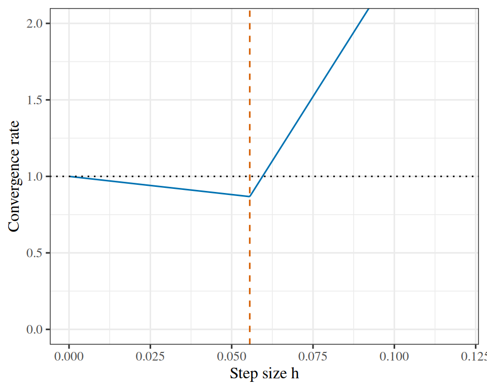
7.1 Exact line search
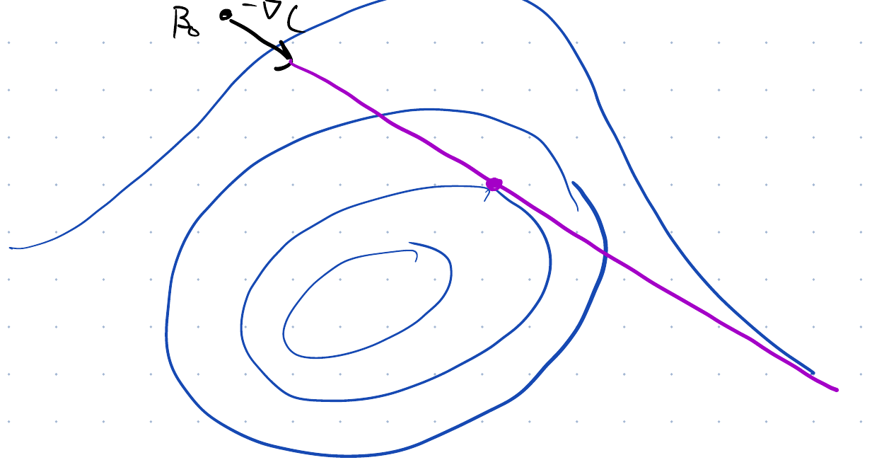
Choosing \(\learnrate\) from Exercise 28 needed the eigenvalues of \(\stprod{\design}\), which we will not have for a general cost. The alternative is to stop choosing \(\learnrate\) in advance and choose it afresh at every step, by minimizing along the ray the gradient points down:
\[\learnrate_t = \argmin_{\learnrate}\; C\paren{\vcoef_t - \learnrate\grad C(\vcoef_t)}\]
Exercise 40 (Choose the step size by minimizing along the ray)
Exercise 40 (Choose the step size by minimizing along the ray) Instead of fixing \(\learnrate\) in advance, pick the best one at every step:
\[\learnrate_t = \argmin_{\learnrate}\; C\paren{\vcoef_t - \learnrate\grad C(\vcoef_t)}\]
This is exact line search. It reduces a search over \(\reals^{\ninputvars+1}\) to a search over a single variable, which for a quadratic can be done in closed form.
Write \(\vg = \grad J(\vcoef_t)\) and \(\vr = \design\vcoef_t - \vy\). Expand \(J(\vcoef_t - \learnrate\vg)\) as a quadratic in \(\learnrate\).
Solution 40. \(\design(\vcoef_t - \learnrate\vg) - \vy = \vr - \learnrate \design\vg\), so
\[ \begin{aligned} J(\vcoef_t - \learnrate\vg) &= \norm{\vr - \learnrate \design\vg}_2^2 \\ &= \norm{\vr}_2^2 - 2\learnrate\,\vr^\top \design\vg + \learnrate^2\norm{\design\vg}_2^2 \end{aligned} \]
a parabola in \(\learnrate\), opening upward whenever \(\design\vg \ne \vzero\).
Exercise 41 (Choose the step size by minimizing along the ray (part 2))
Exercise 41 (Choose the step size by minimizing along the ray (part 2)) Use the setup of Exercise 40.
Minimize it over \(\learnrate\), and use \(\vg = 2\tp{\design} \vr\) to simplify the answer to
\[\learnrate_t = \frac{\norm{\vg}_2^2}{2\norm{\design\vg}_2^2}\]
Solution 41. Differentiate and set to zero:
\[-2\,\vr^\top \design\vg + 2\learnrate\norm{\design\vg}_2^2 = 0 \quad\Longrightarrow\quad \learnrate_t = \frac{\vr^\top \design\vg}{\norm{\design\vg}_2^2}\]
The numerator simplifies, because \(\vr^\top \design\vg = (\tp{\design}\vr)^\top \vg\) and \(\tp{\design} \vr = \tfrac{1}{2}\vg\):
\[ \begin{aligned} \vr^\top \design\vg &= \tfrac{1}{2}\dprod{\vg}{\vg} \\ &= \tfrac{1}{2}\norm{\vg}_2^2 \end{aligned} \]
giving \(\learnrate_t =\norm{\vg}_2^2 / \paren{2\norm{\design\vg}_2^2}\). Both quantities are already computed on the way to the gradient, so the exact step costs one extra matrix–vector product.
Exercise 42 (Choose the step size by minimizing along the ray (part 3))
Exercise 42 (Choose the step size by minimizing along the ray (part 3)) Use the setup of Exercise 40.
Compute \(\learnrate_t\) at \(\vcoef_0 = (0,0)^\top\) for our three points, in exact fractions.
Solution 42. At \(\vcoef_0 = \vzero\), Exercise 10 found \(\vg = (-14, -18)^\top\) and \(\vr = (-1,-3,-3)^\top\).
\[ \begin{aligned} \norm{\vg}_2^2 &= 196 + 324 \\ &= 520, \end{aligned} \qquad \design\vg = \sbmat{ -14 \\ -32 \\ -50 }, \qquad \begin{aligned} \norm{\design\vg}_2^2 &= 196 + 1024 + 2500 \\ &= 3720 \end{aligned} \]
\[ \begin{aligned} \learnrate_0 &= \frac{520}{2 \cdot 3720} \\ &= \frac{520}{7440} \\ &= \frac{13}{186} \\ &\approx 0.0699 \end{aligned} \]
Exercise 43 (Choose the step size by minimizing along the ray (part 4))
Exercise 43 (Choose the step size by minimizing along the ray (part 4)) Use the setup of Exercise 40.
Compute \(\vcoef_1\) and \(J(\vcoef_1)\), in exact fractions.
Solution 43. \[ \begin{aligned} \vcoef_1 &= -\learnrate_0\vg \\ &= \tfrac{13}{186}(14, 18)^\top \\ &= \paren{\tfrac{91}{93},\, \tfrac{39}{31}}^\top \\ &\approx (0.978,\ 1.258)^\top \end{aligned} \]
\[ \begin{aligned} J(\vcoef_1) &= 19 - 2\learnrate_0(260) + \learnrate_0^2(3720) \\ &= \tfrac{77}{93} \\ &\approx 0.828 \end{aligned} \]
Exercise 44 (Choose the step size by minimizing along the ray (part 5))
Exercise 44 (Choose the step size by minimizing along the ray (part 5)) Use the setup of Exercise 40.
Compare with the three constant steps of Exercise 10.
Solution 44. Against the constant steps, after a single step:
| step rule | \(\learnrate\) | \(J(\vcoef_1)\) |
|---|---|---|
| constant | \(1/20 = 0.050\) | \(2.30\) |
| exact line search | \(13/186 \approx 0.070\) | \(\mathbf{0.828}\) |
| constant | \(1/10 = 0.100\) | \(4.20\) |
| constant | \(3/20 = 0.150\) | \(24.70\) |
The minimum is \(J(\vcoef^\star) = 2/3 \approx 0.667\), so one exact step has already removed most of the difference from the minimum. The chosen \(\learnrate\) lands between the two constant steps that worked — it is not simply “as large as possible”.
Exercise 45 (Choose the step size by minimizing along the ray (part 6))
Exercise 45 (Choose the step size by minimizing along the ray (part 6)) Use the setup of Exercise 40.
Show that consecutive exact-line-search directions are orthogonal: \(\dprod{\grad J(\vcoef_{t+1})}{\grad J(\vcoef_t)} = 0\).
Solution 45. \(\learnrate_t\) minimizes \(\linefn(\learnrate) = J(\vcoef_t - \learnrate\vg_t)\), so \(\linefn'(\learnrate_t) = 0\). By the chain rule,
\[\linefn'(\learnrate) = -\dprod{\grad J(\vcoef_t - \learnrate\vg_t)}{\vg_t}\]
and at \(\learnrate = \learnrate_t\) the first factor is \(\grad J(\vcoef_{t+1})\), so \(\dprod{\grad J(\vcoef_{t+1})}{\grad J(\vcoef_t)} = 0\).
Exercise 46 (Choose the step size by minimizing along the ray (part 7))
Exercise 46 (Choose the step size by minimizing along the ray (part 7)) Use the setup of Exercise 40.
What does that say the path looks like in a long thin valley?
Solution 46. So every step is at right angles to the one before it, and the path has a staircase shape. In a long thin valley that is a disadvantage: the alternating right-angle turns make the iterates zig-zag across the valley while advancing very little along it, which is the same \(\condnum\)-dependent slowness as Exercise 33. Choosing the best step along each ray does not fix a badly conditioned problem; it just stops you overshooting while you progress slowly.
Exercise 47 (Choose the step size by minimizing along the ray (part 8))
Exercise 47 (Choose the step size by minimizing along the ray (part 8)) Use the setup of Exercise 40.
Give the reason exact line search is rarely used in practice, even though it is the best step along the ray.
Solution 47. Because the closed form in Solution 41 exists only for a quadratic. For anything else — logistic regression, a neural network — \(\argmin_\learnrate\) is itself an optimization problem, solved approximately by repeatedly evaluating \(C\), and each evaluation is a full pass over the data. Spending several passes to perfect one step is a wasteful use of computation when an approximate step costs one pass and gets most of the benefit.
Exercise 48 does this: it asks for enough decrease rather than the most.
7.2 Backtracking line search
Exact line search is too expensive away from the quadratic case, so in practice we settle for a step that is good enough rather than best. Start at \(\learnrate = 1\), evaluate the cost there, accept if the decrease is large enough, and otherwise shrink \(\learnrate\) and try again.
This is backtracking line search, and “large enough” is the Armijo condition that Exercise 48 works through.
Line search and step-size selection are covered properly in chapter 9 of Convex Optimization by Stephen Boyd and Lieven Vandenberghe, which is freely readable at https://web.stanford.edu/~boyd/cvxbook/. Section 9.2, “Descent methods”, sets out both line searches used here; section 9.3, “Gradient descent method”, gives the convergence rate in terms of the condition number that Exercise 34 derives; and section 9.4, “Steepest descent method”, takes up the dependence on the choice of norm that Exercise 5 raises.
Exercise 48 (Backtracking: ask for enough decrease, not the most)
Exercise 48 (Backtracking: ask for enough decrease, not the most) Backtracking line search starts with a large step and shrinks it until the step is good enough. “Good enough” is the Armijo condition: for a fixed \(\armijo \in (0,1)\),
\[C\paren{\vcoef_t - \learnrate\grad C} \;\le\; C(\vcoef_t) - \armijo\,\learnrate\,\norm{\grad C}_2^2\]
Start at \(\learnrate = 1\) and shrink by a fixed factor until it holds.
The right-hand side is the linear prediction of where the cost would go, discounted by \(\armijo\). Say what the condition is comparing, and why \(\armijo = 1\) would be the wrong thing to ask for.
Solution 48. It compares the decrease we actually got against the decrease the linear model of the cost predicted. Stepping \(\learnrate\) along \(-\grad C\) should, to first order, lower the cost by \(\learnrate\norm{\grad C}_2^2\) — that is the first-order term of Exercise 5 with the step length put back in. The condition accepts \(\learnrate\) when the real decrease is at least the fraction \(\armijo\) of the predicted one.
Asking for \(\armijo = 1\) would demand the full linear prediction. A convex cost lies above its tangent line, so the real decrease is strictly less than the predicted decrease for every \(\learnrate > 0\), no step is ever accepted, and the line search keeps rejecting steps. It shrinks \(\learnrate\) toward zero and makes no progress. Our least-squares cost is convex, so this is what happens here.
A non-convex cost can curve the other way and beat its tangent line over some range of \(\learnrate\), so \(\armijo = 1\) would not reject every step there. It would still be a bad choice: acceptance would then depend on the local curvature rather than on the step being good, which is the opposite of what a line-search condition is for.
Exercise 49 (Backtracking: ask for enough decrease, not the most (part 2))
Exercise 49 (Backtracking: ask for enough decrease, not the most (part 2)) Use the setup of Exercise 48.
Run the search at \(\vcoef_0 = (0,0)^\top\) on our three points with \(\armijo = 10^{-4}\), starting at \(\learnrate = 1\) and shrinking by \(1/10\). Use \(J(\vcoef_0) = 19\) and \(\norm{\grad J}_2^2 = 520\), and note that \(\learnrate = 1\) gives \(J = 3219\).
Solution 49. The required decrease is \(\armijo \learnrate \cdot 520 = 0.052\learnrate\), so the test is \(J(\vcoef_1) \le 19 - 0.052\learnrate\).
| trial | \(\learnrate\) | \(J(\vcoef_1)\) | required \(\le\) | verdict |
|---|---|---|---|---|
| 1 | \(1\) | \(3219\) | \(18.948\) | reject |
| 2 | \(1/10\) | \(4.20\) | \(18.995\) | accept |
Exercise 50 (Backtracking: ask for enough decrease, not the most (part 3))
Exercise 50 (Backtracking: ask for enough decrease, not the most (part 3)) Use the setup of Exercise 48.
Which \(\learnrate\) is accepted?
Solution 50. So \(\learnrate = 1/10\) is accepted. The first trial fails badly — starting from \(\vcoef_0 = (0,0)\), a full step lands at \((14, 18)\) — and the second is accepted immediately. With \(\armijo\) this small the condition is doing little more than insisting the cost went down at all.
Exercise 51 (Backtracking: ask for enough decrease, not the most (part 4))
Exercise 51 (Backtracking: ask for enough decrease, not the most (part 4)) Use the setup of Exercise 48.
Repeat with \(\armijo = 1/2\). You will need \(J = 14.172\) at \(\learnrate = 1/100\).
Solution 51. Now the required decrease is \(0.5 \cdot 520 \cdot \learnrate = 260\learnrate\).
| trial | \(\learnrate\) | \(J(\vcoef_1)\) | required \(\le\) | verdict |
|---|---|---|---|---|
| 1 | \(1\) | \(3219\) | \(-241\) | reject |
| 2 | \(1/10\) | \(4.20\) | \(-7\) | reject |
| 3 | \(1/100\) | \(14.172\) | \(16.4\) | accept |
The first two fail for an interesting reason: the value they demand is below the smallest \(J\) can ever take, so no cost surface could have satisfied them. The strict \(\armijo\) has driven the accepted step down to about a seventh of the one exact line search chose.
Exercise 52 (Backtracking: ask for enough decrease, not the most (part 5))
Exercise 52 (Backtracking: ask for enough decrease, not the most (part 5)) Use the setup of Exercise 48.
Show that with \(\armijo = 1/2\) no step longer than about \(0.0705\) can ever be accepted from this starting point, whatever the shrink factor.
Solution 52. The cost can never fall below \(J(\vcoef^\star) = 2/3\), so the largest decrease available from \(J = 19\) is \(19 - 2/3 = 55/3\). The Armijo condition with \(\armijo = 1/2\) demands a decrease of \(260\learnrate\), which is achievable only if
\[260\learnrate \le \tfrac{55}{3} \quad\Longrightarrow\quad \learnrate \le \tfrac{55}{780} = \tfrac{11}{156} \approx 0.0705\]
Any longer step is rejected no matter what the cost surface does, because the demand is impossible rather than merely unmet.
Exercise 53 (Backtracking: ask for enough decrease, not the most (part 6))
Exercise 53 (Backtracking: ask for enough decrease, not the most (part 6)) Use the setup of Exercise 48.
Compare that number with the exact-line-search step of Exercise 40.
Solution 53. That bound is a quick one, obtained from the lower bound of \(J\) alone. The quadratic gives the exact answer, and it is simpler. Writing the decrease from Exercise 40 as \(\learnrate\norm{\vg}_2^2 - \learnrate^2\norm{\design\vg}_2^2\), the Armijo condition reads
\[\learnrate\norm{\vg}_2^2 - \learnrate^2\norm{\design\vg}_2^2 \;\ge\; \armijo \learnrate\norm{\vg}_2^2 \quad\Longleftrightarrow\quad \learnrate \;\le\; 2(1-\armijo)\,\learnrate^\star\]
So on a quadratic, \(\armijo = 1/2\) is exactly the demand that the step be no longer than the exact minimizer \(\learnrate^\star = 13/186 \approx 0.0699\), and the floor derived in Solution 52 was within one percent of it. Smaller \(\armijo\) relaxes the ceiling proportionally: \(\armijo = 10^{-4}\) allows almost twice \(\learnrate^\star\), so Solution 49 accepted \(\learnrate = 1/10\).
Exercise 54 (Backtracking: ask for enough decrease, not the most (part 7))
Exercise 54 (Backtracking: ask for enough decrease, not the most (part 7)) Use the setup of Exercise 48.
What does a small \(\armijo\) gain, and what does it risk?
Solution 54. A small \(\armijo\) allows long steps. The test is nearly “did the cost go down”, so backtracking stops at the first trial that works and makes fast progress per iteration.
The risk is that it accepts steps that make very little progress relative to their length, since a step that barely decreases the cost still passes when \(\armijo\) is tiny. In the worst case the iterates can progress slowly, making vanishing improvements while never triggering a rejection, and convergence guarantees are lost. The usual compromise is \(\armijo = 10^{-4}\) with a shrink factor of \(1/2\) rather than \(1/10\), which keeps the steps long while shrinking gently enough not to overshoot a good step size on the way down.
Watch
- Weinberger discusses how to choose the step size, from 23:20 [2], Lecture 12.
- He then compares gradient descent with Newton’s method, from 35:10.
8 Knowing when to stop
Three quantities are worth watching as the iterations run:
- the cost;
- the parameters;
- the size of the gradient.
The usual rule watches the cost, relative to its own size.
Definition 6 (Relative change stopping criterion)
Definition 6 (Relative change stopping criterion) The relative change stopping criterion with tolerance \(\text{tol} > 0\) stops gradient descent at the first step \(t\) for which
\[\frac{\abs{C(\vcoef_{t+1}) - C(\vcoef_t)}}{\abs{C(\vcoef_t)}} < \text{tol}.\]
Example 11 (Stopping a descent on \(C(\regcoef) = \regcoef^2 + 1\))
Example 11 (Stopping a descent on \(C(\regcoef) = \regcoef^2 + 1\)) Run gradient descent from \(\regcoef_0 = 2\) with \(\learnrate = 0.25\), and stop at tolerance \(\text{tol} = 0.01\):
[1] 5.000000000 0.002918288The criterion stops at step \(t = 5\), where the update to \(\regcoef_{t+1} = 0.031\) changes the cost by a relative 0.0029. That parameter is still not the minimizer \(0\): a small relative change in cost does not show that the parameter has stopped moving.
Exercise 55 (Decide when to stop)
Exercise 55 (Decide when to stop) There is no step at which gradient descent reports that it has converged, so we need a rule. The usual one watches the relative decrease in cost:
\[\frac{\abs{C(\vcoef_{t+1}) - C(\vcoef_t)}}{\abs{C(\vcoef_t)}} < \text{tol}\]
Compute this quantity for the first step of Exercise 11 at \(\learnrate = 1/20\), and say whether a tolerance of \(10^{-5}\) would have stopped there.
Solution 55. \(C\) went from \(19\) to \(23/10 = 2.3\), so
\[\frac{|2.3 - 19|}{19} = \frac{16.7}{19} \approx 0.879\]
Nowhere near \(10^{-5}\), so the rule keeps going — as it should, since \(J = 2.3\) is still more than three times the minimum \(2/3\).
Exercise 56 (Decide when to stop (part 2))
Exercise 56 (Decide when to stop (part 2)) Use the setup of Exercise 55.
Why divide by \(|C(\vcoef_t)|\) at all?
Solution 56. To make the rule scale-free. An absolute threshold depends on the units of the response, which have nothing to do with whether the fit has converged. Dividing by \(|C(\vcoef_t)|\) removes the units, so the rule asks the question a person actually has in mind: is the cost still moving by a meaningful fraction of itself?
Exercise 57 (Decide when to stop (part 3))
Exercise 57 (Decide when to stop (part 3)) Use the setup of Exercise 55.
Give a specific change to the problem that leaves the fit identical but changes the absolute decrease.
Solution 57. Multiply every \(y_i\) by \(1000\) — change the units of the response from metres to millimetres — and the fitted line is the same line in new units, but every cost is a million times larger and so is every absolute decrease. An absolute threshold would stop far too early in one unit system and far too late in the other, and nothing about the problem has changed.
Exercise 58 (Decide when to stop (part 4))
Exercise 58 (Decide when to stop (part 4)) Use the setup of Exercise 55.
A common choice is \(\text{tol} \approx 1/\sqrt{\nobs}\). Argue for it from what the cost is estimating, rather than from convention.
Solution 58. The cost is a sum, or average, over a finite sample of size \(n\), and what we care about is the population quantity it estimates. That estimate carries sampling error of order \(1/\sqrt{\nobs}\): draw a different sample of the same size and the whole cost surface shifts by about that much, taking its minimizer with it.
So improvements in the training cost that are much smaller than \(1/\sqrt{\nobs}\) are not improvements in anything we can measure on new data. They are adjustments to the noise in this particular sample, which is overfitting. Setting \(\text{tol} \approx 1/\sqrt{n}\) stops optimizing once the arithmetic gets finer than the data can justify.
This is a rough guide, not a theorem: the constant in front depends on the variance of the loss, and the \(10^{-5}\) in the notes is the same idea with \(n\) around \(10^{10}\), or simply a number someone found worked.
Exercise 59 (Decide when to stop (part 5))
Exercise 59 (Decide when to stop (part 5)) Use the setup of Exercise 55.
Two other quantities could be watched instead: the size of the step \(\norm{\vcoef_{t+1} - \vcoef_t}\), and the size of the gradient \(\norm{\grad C(\vcoef_t)}\). Say what each one is good at and how each can mislead.
Solution 59. Step size \(\norm{\vcoef_{t+1} - \vcoef_t}\). Good when what you care about is the parameters themselves — a coefficient you intend to report and interpret. It misleads when the cost is flat in some direction: the iterates can move a long way along the bottom of a valley while the fit barely changes, which reads as “still working” when the useful work has finished. For constant-step descent it is exactly \(\learnrate\norm{\grad C(\vcoef_t)}\), so it inherits the properties of the gradient criterion as well, scaled by \(\learnrate\).
Gradient size \(\norm{\grad C(\vcoef_t)}\). This measures distance to the condition we are actually solving — a vanishing gradient — rather than progress between two arbitrary iterates, and the cost criterion cannot do that at all: the cost keeps falling by less and less without ever telling you how far from stationary you are. It misleads in two ways: it is not scale-free either, and it cannot tell a minimum from a saddle point or a flat plateau, where the gradient is small and the cost is not near its lowest value.
In practice, check more than one. The relative-decrease rule alone cannot distinguish “converged” from “taking tiny steps”.
Exercise 60 (Decide when to stop (part 6))
Exercise 60 (Decide when to stop (part 6)) Use the setup of Exercise 55.
The Week 6 notes add the warning “don’t use for neural networks (danger!)”. Explain what goes wrong there.
Solution 60. A neural network’s cost is not convex, and its descent path typically spends long stretches on plateaus where the cost moves very little and then falls sharply. A small relative decrease is therefore evidence of a plateau, not of a minimum, and stopping on it abandons training at a point whose only property is being flat.
Two more reasons in the same direction. Neural networks are trained with stochastic gradients (Exercise 67), so consecutive costs differ by sampling noise from the minibatch as much as by progress, and the ratio is dominated by that noise. And they are usually meant to be stopped early, on a validation metric rather than a training cost — the training cost will happily keep falling while the model gets worse on new data.
The standard practice is to stop on validation performance, or simply on a fixed budget of epochs, and to treat the training curve as a diagnostic.
9 The cost of a step
Everything so far has counted iterations. The total cost is the number of iterations times the cost of one. The rest of the chapter is motivated by that per-iteration cost.
Exercise 61 (Count what a step costs)
Exercise 61 (Count what a step costs) Express the cost as a sum over the training points,
\[C(\vcoef) = \sumin \ell_i(\vcoef)\]
where \(\ell_i\) is the loss on point \(i\) — squared error, logistic loss, or anything else.
How many arithmetic operations does one evaluation of \(\grad C\) take, in terms of \(\nobs\) and \(\ninputvars\)?
Solution 61. \(O(n\ninputvars)\).
The gradient of a sum is the sum of the gradients, so \(\grad C = \sumin \grad \ell_i\) — \(n\) terms, and each has to be computed and added.
Note this is \(O(n)\) in the number of terms — the form the Week 6 notes give — with the \(\ninputvars\) made explicit.
Exercise 62 (Count what a step costs (part 2))
Exercise 62 (Count what a step costs (part 2)) Use the setup of Exercise 61.
State any assumption you make about \(\grad \ell_i\).
Solution 62. The assumption is that one \(\grad \ell_i\) costs \(O(\ninputvars)\), which holds for every model in this course that puts \(\vcoef\) into the loss through the single inner product \(\dprod{\vcoef}{\vx_i}\): least squares, logistic regression, support vector machines. Forming that inner product is \(\ninputvars\) multiplications, and the chain rule turns the scalar derivative into a vector by scaling \(\vx_i\), another \(\ninputvars\).
Exercise 63 (Count what a step costs (part 3))
Exercise 63 (Count what a step costs (part 3)) Use the setup of Exercise 61.
Give the total cost of running \(T\) gradient-descent steps.
Exercise 64 (Count what a step costs (part 4))
Exercise 64 (Count what a step costs (part 4)) Use the setup of Exercise 61.
Compare the cost with solving the normal equations directly.
Solution 64. Solving the normal equations costs \(O(n\ninputvars^2)\) to form \(\stprod{\design}\) plus \(O(\ninputvars^3)\) to factor it.
Exercise 65 (Count what a step costs (part 5))
Exercise 65 (Count what a step costs (part 5)) Use the setup of Exercise 61.
For which shapes of data is each faster?
Solution 65.
- Small \(\ninputvars\), any \(n\): the direct solve wins outright. With \(\ninputvars = 10\) the cube is trivial, and the \(O(n\ninputvars^2)\) pass is a single pass over the data where descent needs \(T\) of them.
- Large \(\ninputvars\): descent wins, because \(n\ninputvars^2\) and \(\ninputvars^3\) both grow faster in \(\ninputvars\) than \(n\ninputvars T\) does. With \(\ninputvars = 10^5\), \(\ninputvars^3\) is \(10^{15}\) operations and \(\stprod{\design}\) is a \(10^{10}\)-entry matrix that will not fit in memory, while a gradient step never forms it. Which of the two terms dominates the direct solve depends on \(n\) against \(\ninputvars\): the cube leads when \(n \lesssim \ninputvars\), and the \(O(n\ninputvars^2)\) pass leads otherwise.
- No closed form: the comparison does not arise, and descent is the only option — which is the case for every model after this chapter.
The crossover is roughly \(T\) against \(\ninputvars\): iterate when you expect fewer steps than you have features.
Exercise 66 (Count what a step costs (part 6))
Exercise 66 (Count what a step costs (part 6)) Use the setup of Exercise 61.
Suppose \(\nobs = 10^{8}\) and you want \(1000\) steps. How many passes over the data is that, and why does that number force a method that does not read all of it before each step?
Solution 66. One gradient evaluation touches all \(10^8\) points, so \(1000\) steps is \(1000\) passes over the data — \(10^{11}\) gradient computations before the first answer.
That is the number that makes full-batch descent unusable at scale. The work is spent re-reading data that has not changed to compute a direction that changes only slightly, and the fix is to stop insisting on the exact gradient: sample it instead, which is Stochastic gradient descent.
Remark 1 (How gradient descent relates to Newton’s method)
Remark 1 (How gradient descent relates to Newton’s method). Gradient descent steps along \(-\grad C(\vcoef_{t-1})\), scaled by a step size \(\learnrate\) that you choose. Here \(\grad C\) is the gradient of the cost. Newton’s method steps along \(-\hessf{\vcoef_{t-1}}^{-1} \grad C(\vcoef_{t-1})\). It replaces the scalar \(\learnrate\) with the inverse of the Hessian of \(C\), which sets both the direction and the length of the step. The Newton-Raphson algorithm in the statistics notes is the same method, applied to the gradient of the negative log-likelihood.
Newton’s method needs no step size, and it reaches the minimizer of a quadratic cost in one step. Each step costs more, because it forms a \(D \times D\) matrix and solves a linear system with it, where a gradient step only needs the gradient. Logistic regression works this comparison through on a fitted model.
10 Stochastic gradient descent
A full gradient is an average over the whole training set. An average over a set of points is exactly the thing statistics has a standard answer for: estimate it from a sample of the points. Stochastic gradient descent takes that literally. At each step, it draws one training point at random and steps along its gradient, as though the training set consisted of that point alone.
Definition 7 (Stochastic gradient descent)
Definition 7 (Stochastic gradient descent) Stochastic gradient descent (SGD) [12] is gradient descent that replaces the gradient of the cost by the gradient of one training point, chosen at random. Let the cost be the mean of the point losses, \(C(\vcoef) = \avgin \ell_i(\vcoef)\). At step \(t\), draw an index \(I_t \sim \text{Uniform}\{1, \ldots, n\}\) and update:
\[\vd_t = -\grad \ell_{I_t}(\vcoef_t), \qquad \vcoef_{t+1} = \vcoef_t + \learnrate_t \vd_t.\]
Example 12 (The three possible stochastic steps)
Example 12 (The three possible stochastic steps) Use the three points of Exercise 10, with the squared-error loss \(\ell_i(\vcoef) = (\coef{0} + \coef{1} x_i - y_i)^2\). Its gradient is \(\grad \ell_i(\vcoef) = 2(\coef{0} + \coef{1} x_i - y_i)\,(1, x_i)\). From \(\vcoef_0 = \vzero\) with \(\learnrate = 0.1\), compute the update for each possible draw of \(I_0\):
import numpy as np

x_sgd = np.array([0.0, 1.0, 2.0])
y_sgd = np.array([1.0, 3.0, 3.0])
beta_sgd0 = np.zeros(2)
h_sgd = 0.1

def point_grad(beta, i):
    return 2 * (beta[0] + beta[1] * x_sgd[i] - y_sgd[i]) * np.array([1.0, x_sgd[i]])

for i in range(3):
    print(i + 1, beta_sgd0 - h_sgd * point_grad(beta_sgd0, i))
1 [0.2 0. ]
2 [0.6 0.6]
3 [0.6 1.2]The update depends on which point is drawn: the first point pulls only the intercept, and the second and third pull both coefficients. Each draw gives a different step.
The direction is wrong at every step and correct on average, and that is enough. This idea is older than machine learning. Herbert Robbins and Sutton Monro published it in 1951 as a way of finding the root of a function that can only be observed with noise [13]. Their conditions on the step sizes are still the ones in use.
Definition 8 (Robbins–Monro conditions)
Definition 8 (Robbins–Monro conditions) The Robbins–Monro conditions [13] on the step sizes \(\learnrate_1, \learnrate_2, \ldots\) of stochastic gradient descent are
\[\sum_{t=1}^{\infty} \learnrate_t = \infty \qquad\text{and}\qquad \sum_{t=1}^{\infty} \learnrate_t^2 < \infty.\]
The first lets the iterates travel any distance they need to. The second keeps the accumulated noise finite.
Example 13 (Which schedules meet the conditions)
Example 13 (Which schedules meet the conditions) Compare partial sums of the fixed step size \(\learnrate_t = 0.1\) and the decaying step size \(\learnrate_t = 1/t\), up to \(n\) terms:
100 9.999999999999998 1.0000000000000004 5.187377517639621 1.6349839001848931
10000 999.9999999999999 100.00000000000003 9.787606036044382 1.6448340718480599
1000000 100000.00000000003 10000.000000000004 14.392726722865726 1.6449330668487263 [,1] [,2] [,3]
n_terms 100.000000 10000.000000 1.000000e+06
const_sum 10.000000 1000.000000 1.000000e+05
const_sq 1.000000 100.000000 1.000000e+04
inv_sum 5.187378 9.787606 1.439273e+01
inv_sq 1.634984 1.644834 1.644933e+00The sums of \(0.1\) and of \(1/t\) keep growing as \(n\) grows, so both meet the first condition. The sum of squares of \(1/t\) levels off near \(\pi^2/6 \approx 1.645\), so \(1/t\) meets the second condition. The sum of squares of \(0.1\) keeps growing, so the fixed rate fails it.
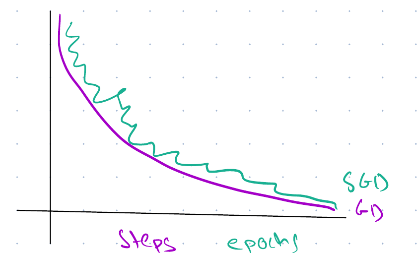
Exercise 67 (Show that one random point points the right way on average)
Exercise 67 (Show that one random point points the right way on average) Express the cost as a sample mean rather than a sum:
\[C(\vcoef) = \avgin \ell_i(\vcoef)\]
At step \(t\), draw an index \(I_t\) uniformly from \(\{1, \ldots, n\}\) and step along that one point’s gradient:
\[\vd_t = -\grad \ell_{I_t}(\vcoef_t), \qquad \vcoef_{t+1} = \vcoef_t + \learnrate_t \vd_t\]
Compute \(\E{\vd_t}\), showing the step where uniformity is used.
Solution 67. \[ \begin{aligned} \E{\vd_t} &= \sumin \Pr[I_t = i]\paren{-\grad \ell_i(\vcoef_t)} \\ &= \sumin \frac{1}{n}\paren{-\grad \ell_i(\vcoef_t)} \\ &= -\avgin \grad \ell_i(\vcoef_t) \\ &= -\grad C(\vcoef_t) \end{aligned} \]
Uniformity enters at the second equality, where every \(\Pr[I_t = i]\) becomes \(1/n\). That makes the average of the per-point gradients come out as the gradient of the average. This is the key step: the \(1/n\) in the sampling distribution is the same \(1/n\) that is in the cost.
Exercise 68 (Show that one random point points the right way on average (part 2))
Exercise 68 (Show that one random point points the right way on average (part 2)) Use the setup of Exercise 67.
What does the answer allow us to conclude about a single step, and what does it not?
Solution 68. It supports a statement about the direction: the stochastic step is an unbiased estimate of the full gradient step, so in expectation the method moves the way gradient descent would.
It does not support any statement about a single step. \(\vd_t\) can point uphill — Exercise 72 builds a case where it must — and the cost can rise for many steps in a row. Unbiasedness says the errors average out over many draws, not that any one draw is good. The practical consequence is that the cost curve of stochastic descent is a noisy band trending downward rather than the monotone curve a full-batch run gives, and that the step size has to shrink over time for the iterates to settle rather than fluctuate around the minimum forever.
Exercise 69 (Show that one random point points the right way on average (part 3))
Exercise 69 (Show that one random point points the right way on average (part 3)) Use the setup of Exercise 67.
Rewrite the cost as the sum \(C(\vcoef) = \sum_i \ell_i(\vcoef)\) instead. With \(\vd_t\) unchanged, what is \(\E{\vd_t}\) now?
Solution 69. Nothing about \(\vd_t\) has changed, so its expectation is still the mean of the per-point gradients — but the cost’s gradient is now the sum:
\[\E{\vd_t} = -\avgin \grad \ell_i = -\frac{1}{n}\grad C(\vcoef_t)\]
The direction is right but the magnitude is off by a factor of \(n\): each step is \(n\) times shorter than it should be.
Exercise 70 (Show that one random point points the right way on average (part 4))
Exercise 70 (Show that one random point points the right way on average (part 4)) Use the setup of Exercise 67.
What must change for the method to behave the same way?
Solution 70. Either scale the estimator, \(\vd_t = -\nobs\grad \ell_{I_t}\), or scale the step size, \(\learnrate_t \to n\learnrate_t\).
The two conventions differ only by that constant, and choosing one and using it consistently matters more than which. Exercise 80 shows what happens when they get mixed.
Exercise 71 (Show that one random point points the right way on average (part 5))
Exercise 71 (Show that one random point points the right way on average (part 5)) Use the setup of Exercise 67.
State the cost of one stochastic step in the notation of Exercise 61, and compare it with a full step.
Solution 71. \(O(\ninputvars)\) — one point’s gradient, independent of \(\nobs\). A full step is \(O(n\ninputvars)\), so a stochastic step is \(n\) times cheaper, and in the time one full step takes we can make \(n\) stochastic ones.
For the \(n = 10^{8}\) of Exercise 61, that is the difference between \(1000\) full passes and a single pass that has already taken \(10^{8}\) steps. The estimate of each direction is far worse; there are vastly more of them.
Exercise 72 (Build a step that certainly goes uphill)
Exercise 72 (Build a step that certainly goes uphill) Take the three points again, with \(\ell_i(\vcoef) = (\dprod{\vcoef}{\vx_i} - y_i)^2\) the loss at point \(i\) and \(J(\vcoef) = \tfrac{1}{2}\sumto{i}{3}\ell_i(\vcoef)\) the cost this chapter has been minimizing throughout.
Compute \(\grad \ell_1\), \(\grad \ell_2\), \(\grad \ell_3\) at \(\vcoef_0 = (0,0)^\top\), and check them against \(\grad J(\vcoef_0) = (-14, -18)^\top\) from Exercise 10.
Solution 72. \(\grad \ell_i = 2(\dprod{\vcoef}{\vx_i} - y_i)\vx_i\), and at \(\vcoef_0 = \vzero\) the predictions are all zero, so the residuals are \(-1, -3, -3\):
\[\grad \ell_1 = 2(-1)\sbmat{1\\0} = \sbmat{-2\\0}, \quad \grad \ell_2 = 2(-3)\sbmat{1\\1} = \sbmat{-6\\-6}, \quad \grad \ell_3 = 2(-3)\sbmat{1\\2} = \sbmat{-6\\-12}\]
Their sum is \((-14, -18)^\top\), which is exactly \(\grad J(\vcoef_0)\). The full gradient is the sum of the per-point gradients, which is the fact Exercise 67 rests on.
Exercise 73 (Build a step that certainly goes uphill (part 2))
Exercise 73 (Build a step that certainly goes uphill (part 2)) Use the setup of Exercise 72.
Now start at the minimizer \(\vcoef^\star = (4/3, 1)^\top\). Compute the three per-point gradients there.
Solution 73. Solving the normal equations by hand gave residuals \(\vy - \design\vcoef^\star = (-1/3, 2/3, -1/3)\) at the optimum. The gradient \(\grad \ell_i = 2(\dprod{\vx_i}{\vcoef} - y_i)\vx_i\) carries the opposite, fitted minus observed sign, so the quantity entering each per-point gradient is \((1/3, -2/3, 1/3)\):
\[\grad \ell_1 = \tfrac{2}{3}\sbmat{1\\0}, \quad \grad \ell_2 = -\tfrac{4}{3}\sbmat{1\\1}, \quad \grad \ell_3 = \tfrac{2}{3}\sbmat{1\\2}\]
Exercise 74 (Build a step that certainly goes uphill (part 3))
Exercise 74 (Build a step that certainly goes uphill (part 3)) Use the setup of Exercise 72.
What is their sum?
Solution 74. Their sum is \(\paren{\tfrac{2}{3} - \tfrac{4}{3} + \tfrac{2}{3},\; 0 - \tfrac{4}{3} + \tfrac{4}{3}}^\top = (0,0)^\top\).
Exercise 75 (Build a step that certainly goes uphill (part 4))
Exercise 75 (Build a step that certainly goes uphill (part 4)) Use the setup of Exercise 72.
Why did it have to be that?
Solution 75. It had to be zero because \(\vcoef^\star\) minimizes \(J\), so \(\grad J(\vcoef^\star) = \vzero\), and the full gradient is that sum. Note what this does not say: no individual \(\grad \ell_i\) is zero. The minimum is where the per-point gradients cancel, not where they vanish. That cancellation is the whole source of the noise in stochastic descent — the individual terms stay large forever, and only their average dies.
Exercise 76 (Build a step that certainly goes uphill (part 5))
Exercise 76 (Build a step that certainly goes uphill (part 5)) Use the setup of Exercise 72.
Starting from \(\vcoef^\star\), take one stochastic step on point \(1\) with \(\learnrate = 1/20\). Compute \(J\) before and after, exactly.
Solution 76. \[ \begin{aligned} \vd &= -\grad \ell_1 \\ &= -\tfrac{2}{3}(1,0)^\top, \end{aligned} \]
so
\[ \begin{aligned} \vcoef_1 &= \vcoef^\star + \tfrac{1}{20}\cdot\paren{-\tfrac{2}{3}}(1,0)^\top \\ &= \paren{\tfrac{4}{3} - \tfrac{1}{30},\; 1}^\top \\ &= \paren{\tfrac{13}{10},\; 1}^\top \end{aligned} \]
Using the identity of Exercise 24 with \(\ve = (-1/30, 0)^\top\):
\[ \begin{aligned} J(\vcoef_1) - J(\vcoef^\star) &= \ve^\top \stprod{\design} \ve \\ &= 3\paren{\tfrac{1}{30}}^2 \\ &= \tfrac{1}{300} \end{aligned} \]
so \(J\) rises from \(\tfrac{2}{3} = \tfrac{200}{300}\) to \(\tfrac{201}{300} = \tfrac{67}{100}\). Checking directly: the residuals at \((13/10, 1)\) are \((3/10, -7/10, 3/10)\), whose squares sum to \(67/100\).
Exercise 77 (Build a step that certainly goes uphill (part 6))
Exercise 77 (Build a step that certainly goes uphill (part 6)) Use the setup of Exercise 72.
Full-batch gradient descent, started at \(\vcoef^\star\), does something different. What, and why?
Solution 77. Nothing at all. \(\grad J(\vcoef^\star) = \vzero\) by Solution 75, so the full-batch update \(\vcoef_1 = \vcoef^\star - \learnrate\grad J(\vcoef^\star)\) leaves \(\vcoef^\star\) exactly where it is. The minimizer is a fixed point of full-batch descent, and is not a fixed point of the stochastic version.
Exercise 78 (Build a step that certainly goes uphill (part 7))
Exercise 78 (Build a step that certainly goes uphill (part 7)) Use the setup of Exercise 72.
Generalize: at the minimizer, is there any index whose stochastic step lowers the cost?
Solution 78. No. At \(\vcoef^\star\) every step strictly increases \(J\), whichever index is drawn. The cost is a strictly convex quadratic with its unique minimum at \(\vcoef^\star\), so any move away from that point raises \(J\) — and no \(\grad \ell_i\) is zero, so every draw produces a move.
Exercise 79 (Build a step that certainly goes uphill (part 8))
Exercise 79 (Build a step that certainly goes uphill (part 8)) Use the setup of Exercise 72.
Given that answer, how should the step size behave as training proceeds?
Solution 79. So stochastic gradient descent does not converge to \(\vcoef^\star\) and stay there. With a constant \(\learnrate\) it reaches a neighbourhood and then fluctuates within it, at a radius set by \(\learnrate\) and by how much the per-point gradients disagree. The fix is to shrink the step as training proceeds, so the fluctuation shrinks with it — \(\learnrate_t \propto 1/t\) is the classical schedule, small enough eventually to settle and large enough for long enough to have got there.
Compare Solution 77: full-batch descent needs no such schedule, because its estimate of the direction gets exactly right at the answer while the stochastic one never does. Reading only part of the data at each step forces the step size to shrink.
Read
GeeksforGeeks explains stochastic gradient descent [14].
10.1 Regularization with stochastic descent
Adding a penalty to the cost is the subject of ridge regression, and it interacts with sampling in a way that is easy to get wrong. The loss term is a sum over data points and so can be sampled; the penalty is a function of \(\vcoef\) alone and so cannot. If the penalty is scaled wrongly, you get a model whose regularization is \(n\) times too strong, not the model you asked for.
Exercise 80 (Add a penalty without making the estimator biased)
Exercise 80 (Add a penalty without making the estimator biased) Regularized training minimizes a data term plus a penalty:
\[C(\vcoef) = \avgin \ell_i(\vcoef) + \regpar R(\vcoef)\]
The penalty \(R\) is a function of \(\vcoef\) alone — it does not depend on any data point — so it cannot be sampled the way the loss can.
Write \(\grad C\).
Solution 80. The gradient is linear, so it splits:
\[\grad C(\vcoef) = \avgin \grad \ell_i(\vcoef) + \regpar\,\grad R(\vcoef)\]
Exercise 81 (Add a penalty without making the estimator biased (part 2))
Exercise 81 (Add a penalty without making the estimator biased (part 2)) Use the setup of Exercise 80.
Look for a stochastic estimator of the form \(\vd_t = -\grad \ell_{I_t}(\vcoef_t) - c\,\grad R(\vcoef_t)\) with \(I_t\) uniform and \(c\) a constant. Compute \(\E{\vd_t}\).
Solution 81. The penalty term is not random — \(R\) does not involve \(I_t\) — so it passes straight through the expectation:
\[ \begin{aligned} \E{\vd_t} &= -\E{\grad \ell_{I_t}} - c\,\grad R \\ &= -\avgin\grad \ell_i - c\,\grad R \end{aligned} \]
using Exercise 67 for the first term.
Exercise 82 (Add a penalty without making the estimator biased (part 3))
Exercise 82 (Add a penalty without making the estimator biased (part 3)) Use the setup of Exercise 80.
Find the \(c\) that makes it unbiased.
Solution 82. Comparing with \(-\grad C\) from Solution 80, the data halves already agree, and the penalty halves agree exactly when
\[\boxed{c = \regpar}\]
So the correct estimator is
\[\vd_t = -\grad \ell_{I_t}(\vcoef_t) - \regpar\,\grad R(\vcoef_t)\]
The penalty gradient is applied in full at every step, unscaled. That is the point worth remembering: the loss is sampled and the penalty is not, because only the loss is a sum over data.
Exercise 83 (Add a penalty without making the estimator biased (part 4))
Exercise 83 (Add a penalty without making the estimator biased (part 4)) Use the setup of Exercise 80.
The Week 6 notes write \(c = \nobs\regpar\). Compute the bias that choice produces, and say by what factor the penalty is over-weighted.
Solution 83. With \(c = n\regpar\),
\[\E{\vd_t} = -\avgin\grad \ell_i - n\regpar\,\grad R = -\grad C - (n-1)\regpar\,\grad R\]
so the bias is \(-(\nobs-1)\regpar \grad R\), and the penalty is over-weighted by a factor of \(n\). The estimator is unbiased only when \(\nobs = 1\).
Equivalently, the method is doing unbiased stochastic descent, but on the wrong objective: it is minimizing \(\frac{1}{\nobs}\sum_i \ell_i + \nobs\regpar R\), a problem whose regularization strength is \(\nobs\) times what was asked for.
A correction to the source notes
The Week 6 notes give this step as \(\vd_t = -\grad \ell_{I_t} - n\regpar\,\grad R\), under the mean-cost convention \(C = \tfrac{1}{n}\sum_i \ell_i + \regpar R\). It is off by a factor of \(\nobs\), as Solution 83 shows, and the line after it in those notes also drops a minus sign from the loss term. The corrected form is \(\vd_t = -\grad \ell_{I_t} - \regpar\,\grad R\).
Exercise 84 (Add a penalty without making the estimator biased (part 5))
Exercise 84 (Add a penalty without making the estimator biased (part 5)) Use the setup of Exercise 80.
Now repeat the whole exercise under the sum convention \(C(\vcoef) = \sumin \ell_i(\vcoef) + \regpar R(\vcoef)\).
Solution 84. Under the sum convention,
\[\grad C = \sumin\grad \ell_i + \regpar\,\grad R\]
The sampled loss gradient still has expectation \(\frac{1}{n}\sum_i \grad \ell_i\), which is \(n\) times too small against a sum, so the loss term needs the factor:
\[\vd_t = -n\,\grad \ell_{I_t}(\vcoef_t) - \regpar\,\grad R(\vcoef_t)\]
Exercise 85 (Add a penalty without making the estimator biased (part 6))
Exercise 85 (Add a penalty without making the estimator biased (part 6)) Use the setup of Exercise 80.
Which term picks up a factor of \(\nobs\), and which does not?
Solution 85. The penalty term is unscaled again, so the factor of \(n\) goes on the sampled loss term only.
Exercise 86 (Add a penalty without making the estimator biased (part 7))
Exercise 86 (Add a penalty without making the estimator biased (part 7)) Use the setup of Exercise 80.
State the rule in one sentence.
Solution 86. The rule in one sentence: the factor of \(n\) belongs to whichever term was sampled, never to the penalty. Under the mean convention nothing needs scaling; under the sum convention the loss does. The check that catches the mistake is the one Solution 83 performs: take the expectation of the step over \(I_t\) and require it to equal \(-\grad C\). The penalty does not depend on \(I_t\), so any scaling error in it survives that expectation untouched and shows up at once as a leftover multiple of \(\grad R\).
What does not work is setting \(n = 1\). The error is a spurious factor of \(n\), and at \(n = 1\) that factor is \(1\), so the correct and the incorrect update coincide and the check passes on both. A test the bug passes is worse than no test.
Exercise 87 (Add a penalty without making the estimator biased (part 8))
Exercise 87 (Add a penalty without making the estimator biased (part 8)) Use the setup of Exercise 80.
Take ridge, \(R(\vcoef) =\norm{\vcoef}_2^2\), with \(\nobs = 10^6\). Describe what a run using \(c = \nobs\regpar\) produces, and say why nothing in the program reports an error.
Solution 87. Ridge has \(\grad R = 2\vcoef\), so the direction carries a term \(-2n\regpar\,\vcoef_t\) instead of \(-2\regpar\,\vcoef_t\). With \(n = 10^6\) the shrinkage toward the origin is a million times too strong, and it overwhelms the single data point’s gradient at every step. The iterates collapse toward \(\vcoef = \vzero\) and stay there: the run produces the null model, predicting a constant regardless of the inputs. Keeping only that term, the iteration is \(\vcoef_{t+1} = (1 - 2nh\regpar)\vcoef_t\), so the magnitude contracts whenever \(0 < 2nh\regpar < 2\): monotonically below \(1\), and with the sign alternating between \(1\) and \(2\). Overshooting the origin is therefore not yet divergence. The run diverges only past \(2nh\regpar > 2\), with \(2nh\regpar = 2\) the boundary at which the iterates flip sign forever at constant size.
Nothing reports an error because nothing is wrong as a program. Every quantity is finite, every array has the right shape, the loop runs to its iteration limit, and the reported training cost decreases — on the objective the code is actually minimizing. The only symptom is a model that underfits badly, which looks exactly like a model whose \(\regpar\) was chosen too large. A practitioner would reach for cross-validation, find that every \(\regpar\) on the grid underfits, and conclude the features are uninformative.
This is the characteristic danger of an estimator bug: it does not crash, it silently minimizes a different objective. The defence is the calculation in Solution 81 — take the expectation of your update and check it against the gradient of the objective you meant to minimize.
10.2 Minibatches
One point per step is the cheapest possible estimate of the gradient and the noisiest. Averaging a handful of points lies between the two extremes, and essentially every real implementation does it.
Definition 9 (Minibatch gradient descent)
Definition 9 (Minibatch gradient descent) Minibatch gradient descent is stochastic gradient descent with \(b\) indices \(B_t\) drawn uniformly and with replacement at each step, and the step taken along their average gradient:
\[\vd_t = -\frac{1}{b}\sum_{i \in B_t} \grad \ell_i(\vcoef_t).\]
The number \(b\) is the batch size. With \(b = 1\) it is stochastic gradient descent, and with \(b = n\) it is full-batch descent in expectation.
Exercise 88 (Weigh a minibatch against a single point)
Exercise 88 (Weigh a minibatch against a single point) In practice neither extreme is used. Let \(\vd_t\) be the direction of minibatch gradient descent (Definition 9), and keep the mean-cost convention of Definition 7.
Show that \(\vd_t\) is unbiased for \(-\grad C\), and that its variance is \(1/b\) times that of the single-point estimator.
Solution 88. Each index is drawn uniformly, so each term has expectation \(-\grad C\) by Exercise 67, and the expectation of an average of \(b\) such terms is the same \(-\grad C\). Averaging cannot change an expectation.
For the variance, the draws are independent, so variances add:
\[ \begin{aligned} \Var{\frac{1}{b}\sum_{i \in B_t}\grad \ell_i} &= \frac{1}{b^2}\cdot b \cdot \Var{\grad \ell_{I}} \\ &= \frac{1}{b}\Var{\grad \ell_{I}} \end{aligned} \]
taking the variance coordinatewise. This is the ordinary \(1/b\) of a sample mean, and it is exactly why \(b\) helps: the direction is no more correct on average, it is just less scattered.
(Sampling \(b\) distinct indices, without replacement, does slightly better: the variance picks up a finite-population correction of \((n-b)/(n-1)\), which is negligible once \(b \ll n\). That correction is not why implementations shuffle the data and slice it into consecutive batches. They do that because shuffling guarantees every observation is used exactly once per epoch, and because a contiguous slice reads from memory in order.)
Exercise 89 (Weigh a minibatch against a single point (part 2))
Exercise 89 (Weigh a minibatch against a single point (part 2)) Use the setup of Exercise 88.
Compute the variance of the single-point estimator at \(\vcoef^\star\) for our three points, coordinate by coordinate, using the per-point gradients of Exercise 73.
Solution 89. From Exercise 73, the per-point gradients at \(\vcoef^\star\) are
\[\grad \ell_1 = \paren{\tfrac{2}{3}, 0}^\top, \quad \grad \ell_2 = \paren{-\tfrac{4}{3}, -\tfrac{4}{3}}^\top, \quad \grad \ell_3 = \paren{\tfrac{2}{3}, \tfrac{4}{3}}^\top\]
Their mean is \(\vzero\), so each variance is just the mean of the squares:
\[ \begin{aligned} \Var{\cdot}_{\text{intercept}} &= \frac{1}{3}\paren{\tfrac{4}{9} + \tfrac{16}{9} + \tfrac{4}{9}} \\ &= \frac{8}{9}, \end{aligned} \qquad \begin{aligned} \Var{\cdot}_{\text{slope}} &= \frac{1}{3}\paren{0 + \tfrac{16}{9} + \tfrac{16}{9}} \\ &= \frac{32}{27} \end{aligned} \]
Both are of order one, at a point where the true gradient is exactly zero. That is the noise floor the schedule of Exercise 79 has to shrink against.
Exercise 90 (Weigh a minibatch against a single point (part 3))
Exercise 90 (Weigh a minibatch against a single point (part 3)) Use the setup of Exercise 88.
One step costs \(O(b\ninputvars)\). For a fixed budget of gradient evaluations, is a large \(b\) or a small \(b\) the better use of the budget, judged on this variance argument alone?
Solution 90. Neither, by this argument. A budget of \(K\) gradient evaluations buys \(K/b\) steps, each with variance \(\varpar/b\). Doubling \(b\) halves the variance per step and halves the number of steps, so the two effects cancel: by this argument the budget is spent equally well either way, and any advantage goes to small \(b\), because more steps means more chances to react to the curvature of the cost, and a step is where progress actually happens.
So the variance argument does not justify minibatching at all. It is worth noticing that, rather than assuming the standard practice must follow from the statistics.
Exercise 91 (Weigh a minibatch against a single point (part 4))
Exercise 91 (Weigh a minibatch against a single point (part 4)) Use the setup of Exercise 88.
Minibatches are nonetheless what everyone uses, and \(b\) between \(32\) and \(512\) is typical. Give the reason, and say why it is not the reason in Exercise 90.
Solution 91. Hardware. Computing \(b\) gradients as one \(b \times \ninputvars\) matrix multiplication is far faster than computing them one at a time, because the arithmetic units are vectorized and the memory is fetched in contiguous blocks — a GPU running \(b = 256\) points may take barely longer than it takes for one. The budget in Solution 90 was counted in gradient evaluations; the budget that matters is counted in seconds, and those two stop being proportional as soon as the hardware can do work in parallel.
So \(b\) is chosen as the largest value that still fully uses the hardware and fits in memory, and then the step size is tuned for it. The typical range of \(32\) to \(512\) is a fact about processors, not about estimators.
A second, smaller reason: the gradient noise itself acts a little like a regularizer, helping the iterates escape sharp minima in non-convex problems. That argues for not making \(b\) too large, and it cuts the opposite way from the hardware. So very large batches often need their own adjustments to work at all.
Watch
- Andrew Ng contrasts batch and stochastic gradient descent, from 42:34 [1], Lecture 2.
- He then describes stochastic gradient descent, from 44:56.
Watch
Hutchinson covers minibatch stochastic gradient descent (19 min) [5].
Read
GeeksforGeeks explains mini-batch gradient descent [16].
10.3 Epochs
Mini-batches are built by shuffling the training set and cutting the shuffled order into consecutive blocks of \(b\).
Definition 10 (Epoch)
Definition 10 (Epoch) An epoch is one complete pass through the training set.
Example 14 (Updates per epoch on the Auto data)
Example 14 (Updates per epoch on the Auto data) The Auto data [17] have 392 complete cars. Count the updates in one epoch for several batch sizes \(b\), when the short last block is kept and when it is dropped:
With \(b = n =\) 392 (full-batch descent), an epoch is one update. With \(b = 32\) it is 13 updates when the last block of 8 cars is kept, and 12 when it is dropped. With \(b = 1\) it is 392 updates. A run reported as 50 epochs therefore means very different numbers of updates depending on \(b\).
In mini-batch descent, an epoch is one exhaustion of the blocks, after which the set is shuffled again and cut afresh. When \(n\) is not a multiple of \(b\) the last block is short, and it is either kept as a smaller batch or dropped. Dropping it is common, because a batch of an unusual size makes the noise of that one step differ from all the others.
The difference between an epoch and an update matters as soon as \(b < n\). Full-batch descent makes one update per epoch, so the two words describe the same event and only one of them is needed. Mini-batch descent makes \(\lfloor n/b \rfloor\) updates per epoch when the short final block is dropped, and \(\lceil n/b \rceil\) when it is kept; a training run is usually reported in epochs while the optimizer is counted in updates. One epoch is almost never enough: with a small \(b\) a model may need many updates across many epochs before the parameters are any good. How many epochs is itself a hyperparameter, and the usual way to set it is to watch a held-out score and stop when it stops improving.
11 Learning rate schedules
A constant step size cannot converge precisely under mini-batch sampling: the gradient noise does not vanish as the optimum is approached, so the iterates end up fluctuating around it. Near a minimum and for small \(\learnrate\), the long-run (stationary) variance of the iterates grows in proportion to \(\learnrate\), so the radius of the fluctuation scales as \(\sqrt{\learnrate}\) (and the excess loss, which is quadratic in that radius, scales as \(\learnrate\)). Shrinking \(\learnrate\) as training proceeds is the standard remedy, and the argument for it is the same at both ends of a run. Early on the steps should be long, because the parameters are far from any good solution and the noise is small next to the distance left to travel. Late on they should be short, because the remaining signal is small next to the noise, and a long step then mostly moves in the wrong direction.
The Robbins–Monro conditions introduced in Section 10 (\(\sum \learnrate_t = \infty\) and \(\sum \learnrate_t^2 < \infty\)) make this requirement precise. A constant \(\learnrate\) satisfies the first and fails the second, so the noise keeps the iterates in a fluctuation of fixed size; a sequence like \(\learnrate_t = \learnrate_0/t\) satisfies both. Several of the five practical schedules below satisfy only one of the two conditions and are used anyway, since a training run of fixed length needs no asymptotic guarantee; the conditions explain why decay is needed at all rather than prescribing a single schedule.
Definition 11 (Piecewise constant schedule)
Definition 11 (Piecewise constant schedule) Let:
- \(\learnrate_0\) be the starting learning rate, and \(\learnrate_t\) the rate at update \(t\);
- \(\decay \in (0, 1)\) be the drop factor;
- \(t_1 < t_2 < \cdots\) be the update counts at which the rate drops.
A piecewise constant schedule multiplies the rate by \(\decay\) at each drop point:
\[\learnrate_t = \learnrate_0\,\decay^{k(t)}, \qquad k(t) = \#\{j : t_j \le t\}.\]
It is the simplest schedule, and still among the most used. Both of the things it asks for, the drop factor and the drop points, can be read off the loss curve of an earlier run.
Example 15 (A ten-fold drop twice)
Example 15 (A ten-fold drop twice) Let:
- \(\learnrate_0\) be the starting learning rate;
- \(\decay\) be the drop factor;
- \(\schedlen\) be the total number of updates.
Drop the rate at a third and at two-thirds of the run:
Take \(\learnrate_0 = 0.1\), \(\decay = 0.1\) and \(\schedlen = 90\). The rate at each of the update counts \(t = 0, 29, 30, 59, 60, 90\) is:
The rate stays fixed between drops and falls by the factor \(\decay\) exactly at \(t = 30\) and \(t = 60\).
Definition 12 (Linear decay)
Definition 12 (Linear decay) Let:
- \(\learnrate_0\) be the starting learning rate, and \(\learnrate_t\) the rate at update \(t\);
- \(\learnrate_\schedlen\) be the final rate;
- \(\schedlen\) be the number of updates over which the rate falls.
Linear decay [19] interpolates the rate between \(\learnrate_0\) and \(\learnrate_\schedlen\) over \(\schedlen\) updates, then holds it at \(\learnrate_\schedlen\):
\[\learnrate_t = (1-\schedfrac)\learnrate_0 + \schedfrac \learnrate_\schedlen \quad \text{for } t \le \schedlen, \qquad \schedfrac = \frac{t}{\schedlen}.\]
Three numbers have to be chosen, and \(\schedlen\) is the inconvenient one, since it fixes the number of updates in advance.
Example 16 (Linear decay between two rates)
Example 16 (Linear decay between two rates) Let:
- \(\learnrate_0\) be the starting learning rate;
- \(\learnrate_\schedlen\) be the final rate;
- \(\schedlen\) be the number of updates over which the rate falls.
Take \(\learnrate_0 = 0.1\), \(\learnrate_\schedlen = 0.001\) and \(\schedlen = 90\). The rate at \(t = 0, 45, 90, 120\) is:
The rate falls by the same amount at each update, then stays at 0.001 after update \(\schedlen\).
Definition 13 (Exponential decay)
Definition 13 (Exponential decay) Let:
- \(\learnrate_0\) be the starting learning rate, and \(\learnrate_t\) the rate at update \(t\);
- \(\decay \in (0, 1)\) be the decay factor.
Exponential decay multiplies the rate by \(\decay\) at every update:
\[\learnrate_t = \learnrate_0\,\decay^t.\]
The rate falls by the same proportion each step rather than by the same amount. It never reaches zero, and \(\decay\) has to be set with the intended number of updates in mind.
Example 17 (The same factor over two run lengths)
Example 17 (The same factor over two run lengths) Let:
- \(\learnrate_0\) be the starting learning rate;
- \(\decay\) be the decay factor.
Compare the rate after a short run with the rate after a long one:
Take \(\learnrate_0 = 0.1\) and \(\decay = 0.99\), and compare the rates at \(t = 1000\) and \(t = 100000\):
After 1000 updates the rate is 4.3e-06, and after 100000 it is 0 in floating-point arithmetic. One factor gives two very different schedules.
Definition 14 (Patience)
Definition 14 (Patience) The patience of a training procedure that watches a held-out score is the number of consecutive evaluations the score may go without improving before the procedure reacts.
Example 18 (Two patiences on the same scores)
Example 18 (Two patiences on the same scores) Let:
- \(n_{\text{up}}\) be the number of evaluations over which the held-out score improves, after which it stays flat;
- \(p_{\text{short}}\) and \(p_{\text{long}}\) be two values of the patience.
Take \(n_{\text{up}} = 8\), \(p_{\text{short}} = 1\) and \(p_{\text{long}} = 5\). The procedure first reacts at evaluation 9 with the short patience, and at evaluation 13 with the long one. A short patience reacts to random variation in the score, and a long one waits through many evaluations that could have been used.
Definition 15 (Performance decay)
Definition 15 (Performance decay) Let:
- \(\learnrate\) be the learning rate;
- \(\decay \in (0, 1)\) be the decay factor;
- \(p\) be the patience.
Performance decay (also called plateau decay) watches a held-out score during training. When the score has not improved for \(p\) evaluations, it multiplies \(\learnrate\) by \(\decay\) and continues. It works like early stopping, but it cuts the learning rate instead of stopping. Unlike the other schedules, it looks at the data, and it needs no fixed number of updates in advance.
Example 19 (Halving the rate after three flat evaluations)
Example 19 (Halving the rate after three flat evaluations) Let:
- \(\learnrate_0\) be the starting learning rate;
- \(\decay\) be the decay factor;
- \(p\) be the patience.
Let the held-out score improve for the first \(8\) of \(15\) evaluations and then stay flat. Take \(\learnrate_0 = 0.1\), \(\decay = 0.5\) and \(p = 3\):
[0.1, 0.1, 0.1, 0.1, 0.1, 0.1, 0.1, 0.1, 0.1, 0.1, 0.05, 0.05, 0.05, 0.025, 0.025]lr_pd <- lr0_pd
best_pd <- -Inf
wait_pd <- 0
rates_pd <- numeric(length(score_pd))
for (i in seq_along(score_pd)) {
if (score_pd[i] > best_pd) {
best_pd <- score_pd[i]
wait_pd <- 0
} else {
wait_pd <- wait_pd + 1
if (wait_pd == patience_pd) {
lr_pd <- lr_pd * decay_pd
wait_pd <- 0
}
}
rates_pd[i] <- lr_pd
}
rates_pd [1] 0.100 0.100 0.100 0.100 0.100 0.100 0.100 0.100 0.100 0.100 0.050 0.050
[13] 0.050 0.025 0.025The rate stays at 0.1 while the score improves. It is cut by the factor \(\decay\) after the third flat evaluation, at evaluation 11, and again every third flat evaluation after that.
Two senses of “plateau”
A plateau of the cost is a region of the parameter space where the surface is flat. Plateau decay (Definition 15) is something else: a plateau in the held-out score as training proceeds, which triggers a cut in the step size. The first is a property of \(J\), and the second is a property of the run.
Definition 16 (Cosine decay)
Definition 16 (Cosine decay) Let:
- \(\learnrate_0\) be the starting learning rate, and \(\learnrate_t\) the rate at update \(t\);
- \(\schedlen\) be the number of updates in the run.
Cosine decay [20] takes the rate from \(\learnrate_0\) down to zero along a half period of a cosine over \(\schedlen\) updates:
\[\learnrate_t = \frac{\learnrate_0}{2}\paren{1 + \cos\frac{\pi t}{\schedlen}}.\]
Its derivative vanishes at both ends and is largest in the middle. The run gets a long stretch of nearly full-length steps, a quick transition, and a long stretch of fine ones.
Example 20 (Cosine decay over a fixed run)
Example 20 (Cosine decay over a fixed run) Let:
- \(\learnrate_0\) be the starting learning rate;
- \(\schedlen\) be the number of updates in the run.
Take \(\learnrate_0 = 0.1\) and \(\schedlen = 90\). The rate at \(t = 0, 15, 45, 75, 90\) is:
The rate is 0.1 at the start, half of that at the midpoint \(t = 45\), and zero at \(t = 90\).
Remark 2 (Restarting the cosine schedule)
Remark 2 (Restarting the cosine schedule). Restarting the schedule periodically is a common variant: jump \(\learnrate\) back to \(\learnrate_0\) and decay again. The argument for it is that the jump can move the iterates out of one basin of attraction and into a better one.
Piecewise constant, exponential, linear and cosine decay, and performance decay each add hyperparameters to a procedure that had one, and none of them can be set from the training loss alone.
Figure 11 compares four of these schedules on one set of axes.
Show code
local({
  # HTML formats get an interactive plotly figure.
  # Handout and other static formats get the same schedules drawn with ggplot2.
  # All four schedules start at initial learning rate 0.1 over a horizon of 100 iterations.
  n_iter <- 100
  iters <- 0:n_iter
  lr_init <- 0.1

  # Piecewise constant drops by a factor of 0.5 at one-third and two-thirds of the run.
  piecewise_factor <- 0.5
  drop_one <- round(n_iter / 3)
  drop_two <- round(2 * n_iter / 3)
  lr_piecewise <- lr_init * (piecewise_factor^((iters >= drop_one) + (iters >= drop_two)))

  # Linear decay interpolates to a final rate of 0.01 over 80 updates and then holds constant.
  sched_len <- 80
  lr_final <- 0.01
  sched_frac <- pmin(iters / sched_len, 1)
  lr_linear <- (1 - sched_frac) * lr_init + sched_frac * lr_final

  # Exponential decay multiplies the learning rate by 0.96 at every update.
  decay_factor <- 0.96
  lr_exponential <- lr_init * (decay_factor^iters)

  # Cosine decay follows a half period of a cosine from the initial rate down to zero over 100 updates.
  lr_cosine <- (lr_init / 2) * (1 + cos(pi * iters / n_iter))

  schedules <- list(
    piecewise = lr_piecewise,
    linear = lr_linear,
    exponential = lr_exponential,
    cosine = lr_cosine
  )
  labels <- c(
    piecewise = "piecewise constant",
    linear = "linear decay",
    exponential = "exponential decay",
    cosine = "cosine decay"
  )
  colors <- c(
    piecewise = "#1f77b4",
    linear = "#2ca02c",
    exponential = "#d95f02",
    cosine = "#e7298a"
  )

  if (knitr::is_html_output()) {
    library(plotly)

    widget <- plot_ly()
    for (nm in names(schedules)) {
      widget <- widget |>
        add_trace(
          x = iters,
          y = schedules[[nm]],
          type = "scatter",
          mode = "lines",
          name = labels[[nm]],
          line = list(
            color = colors[[nm]],
            width = 2,
            shape = if (nm == "piecewise") "hv" else "linear"
          ),
          hovertemplate = paste0(labels[[nm]], "<br>iteration %{x}<br>rate %{y:.4f}<extra></extra>")
        )
    }
    widget <- widget |>
      layout(
        xaxis = list(
          title = "iteration",
          zeroline = FALSE
        ),
        yaxis = list(
          title = "learning rate",
          zeroline = FALSE
        ),
        legend = list(orientation = "h", x = 0.5, xanchor = "center", y = -0.2),
        margin = list(t = 10, b = 90)
      ) |>
      config(displaylogo = FALSE, responsive = TRUE)

    # Attach accessible alt text because a plotly widget has none of its own.
    htmltools::div(
      role = "img",
      `aria-label` = paste(
        "Interactive line plot of four learning rate schedules over 100 iterations from 0.1:",
        "piecewise constant with half-step drops at iterations 33 and 67,",
        "linear decay to 0.01 at iteration 80 then flat,",
        "exponential decay with factor 0.96,",
        "and cosine decay over 100 iterations."
      ),
      widget
    )
  } else {
    library(ggplot2)

    sched_df <- do.call(
      rbind,
      lapply(names(schedules), function(nm) {
        data.frame(
          iteration = iters,
          lr = schedules[[nm]],
          schedule = labels[[nm]]
        )
      })
    )
    sched_df$schedule <- factor(sched_df$schedule, levels = unname(labels))

    ggplot(sched_df, aes(x = iteration, y = lr, colour = schedule)) +
      geom_line(
        data = subset(sched_df, schedule != labels[["piecewise"]]),
        linewidth = 0.7
      ) +
      geom_step(
        data = subset(sched_df, schedule == labels[["piecewise"]]),
        linewidth = 0.7
      ) +
      scale_colour_manual(values = setNames(unname(colors), unname(labels))) +
      labs(
        x = "iteration",
        y = "learning rate",
        colour = NULL
      ) +
      theme(
        legend.position = "bottom"
      )
  }
})Watch
The CS231N lecture on optimization discusses learning rates and their schedules, from 59:17 [21], Lecture 3.
Watch
Hutchinson covers learning rate schedules and adaptive methods (11 min) [5].
Read
GeeksforGeeks explains learning rate decay [22].
12 Momentum and adaptive step sizes
Plain gradient descent has two weaknesses that the earlier sections measured. On a cost whose contours are long, narrow ellipses, the steps zig-zag across the valley and creep along it, at a rate set by the condition number (Exercise 34). And one step size \(\learnrate\) serves every coordinate, though the cost may be steep in some directions and nearly flat in others. Most optimizers used to train neural networks modify the update rule to address one or both.
The next exercise builds two of them and compares them with plain gradient descent on the simplest cost that shows the problem, \(C(\vcoef) = \tfrac{1}{2}(\theta_1^2 + 100\,\theta_2^2)\), whose condition number is \(100\).
Exercise 92 (Two ways to beat the zig-zag)
Exercise 92 (Two ways to beat the zig-zag) Take \(C(\vcoef) = \tfrac{1}{2}(\theta_1^2 + 100\,\theta_2^2)\) with \(\vcoef_0 = (1, 1)\), so \(\grad C(\vcoef) = (\theta_1, 100\,\theta_2)\). Count how many updates each method needs to bring the cost below \(10^{-6}\).
Plain gradient descent with \(\learnrate = 0.019\). That is just under the largest step, \(2/100\), that converges on this cost.
Solution 92.
import numpy as np

# The cost 0.5 * (theta_1^2 + 100 * theta_2^2) and its gradient.
KAPPA = 100.0

def cost(theta):
    return 0.5 * (theta[0] ** 2 + KAPPA * theta[1] ** 2)

def grad(theta):
    return np.array([theta[0], KAPPA * theta[1]])

def updates_needed(step, state, goal=1e-6, cap=5000):
    # Run one update rule from (1, 1) until the cost drops below goal; the
    # cap stops a method that never gets there from looping forever.
    theta = np.array([1.0, 1.0])
    for t in range(1, cap + 1):
        theta, state = step(theta, state, t)
        if cost(theta) < goal:
            return t
    return None

def plain(theta, state, t, h=0.019):
    return theta - h * grad(theta), state

zero = np.zeros(2)
print("plain gradient descent:", updates_needed(plain, None))
plain gradient descent: 343# The cost 0.5 * (theta_1^2 + 100 * theta_2^2) and its gradient.
kappa <- 100
cost <- function(theta) 0.5 * (theta[1]^2 + kappa * theta[2]^2)
grad <- function(theta) c(theta[1], kappa * theta[2])
updates_needed <- function(step, state, goal = 1e-6, cap = 5000) {
# Run one update rule from (1, 1) until the cost drops below goal; the
# cap stops a method that never gets there from looping forever.
theta <- c(1, 1)
for (t in seq_len(cap)) {
out <- step(theta, state, t)
theta <- out$theta
state <- out$state
if (cost(theta) < goal) {
return(t)
}
}
NA
}
plain <- function(theta, state, t, h = 0.019) {
list(theta = theta - h * grad(theta), state = state)
}
cat("plain gradient descent:", updates_needed(plain, NULL), "\n")plain gradient descent: 343 Definition 17 (Momentum coefficient)
Definition 17 (Momentum coefficient) Let \(\vg_t\) be the gradient at update \(t\), and \(\vv_t\) a running velocity built from them. The momentum coefficient \(\beta \in [0, 1)\) is the weight on the previous velocity in
\[\vv_t = \beta\,\vv_{t-1} + \vg_t.\]
A gradient from \(k\) updates ago has weight \(\beta^k\), so the velocity remembers roughly the last \(1 / (1 - \beta)\) updates.
Example 21 (How far back the velocity remembers)
Example 21 (How far back the velocity remembers) Let:
- \(\beta\) be the momentum coefficient;
- \(k\) be the number of updates since a gradient was added to the velocity.
For \(\beta = 0, 0.5, 0.9, 0.99\), the weight on a gradient from \(k = 10\) updates ago is \(0, 0.00098, 0.35, 0.9\), and the number of updates remembered, \(1 / (1 - \beta)\), is \(1, 2, 10, 100\) updates. At \(\beta = 0\) the velocity is the current gradient alone, and at \(\beta = 0.99\) it averages over about \(100\) updates.
Definition 18 (Momentum (heavy-ball method))
Definition 18 (Momentum (heavy-ball method)) Let:
- \(C\) be the cost, and \(\vcoef_t\) the parameter vector after update \(t\);
- \(\learnrate\) be the learning rate;
- \(\beta\) be the momentum coefficient.
Momentum (the heavy-ball method) replaces the gradient in the update with a running velocity,
\[\vv_t = \beta\,\vv_{t-1} + \grad C(\vcoef_{t-1}),\]
and steps
\[\vcoef_t = \vcoef_{t-1} - \learnrate\,\vv_t.\]
At \(\beta = 0\) this is plain gradient descent [23].
Example 22 (Momentum on a one-dimensional quadratic)
Example 22 (Momentum on a one-dimensional quadratic) Let:
- \(C(\theta) = \tfrac{1}{2}\theta^2\) be the cost, so \(\grad C(\theta) = \theta\);
- \(\theta_0\) be the starting value of \(\theta\);
- \(\learnrate\) be the learning rate and \(\beta\) the momentum coefficient;
- \(n\) be the number of updates.
Start at \(\theta_0 = 1\) with \(\learnrate = 0.1\), and take \(n = 20\) updates with \(\beta = 0\) and with \(\beta = 0.9\):
After \(n = 20\) updates, plain descent has reached 0.122 and momentum 0.345. Momentum overshoots the minimizer \(0\), down to -0.604 at update 9, and then swings back. On a cost this simple, with a small learning rate, the swing makes momentum slower than plain descent. Its advantage shows on a long, narrow valley, as in the comparison below.
Exercise 93 (Two ways to beat the zig-zag (part 2))
Exercise 93 (Two ways to beat the zig-zag (part 2)) Use the setup of Exercise 92.
Momentum: Keep a running velocity \(\vv_t = \beta\,\vv_{t-1} + \grad C(\vcoef_{t-1})\) and step along it, \(\vcoef_t = \vcoef_{t-1} - \learnrate\,\vv_t\), with \(\vv_0 = \vzero\), \(\beta = 0.9\) and \(\learnrate = 0.01\).
Solution 93.
momentum <- function(theta, v, t, h = 0.01, beta = 0.9) {
  # The velocity accumulates past gradients, so steps along a steady
  # direction grow and steps that keep flipping sign cancel.
  v <- beta * v + grad(theta)
  list(theta = theta - h * v, state = v)
}

cat("momentum:              ", updates_needed(momentum, c(0, 0)), "\n")
momentum: 138 Momentum needs fewer updates than plain gradient descent on this cost. Momentum helps because the steep coordinate \(\theta_2\) keeps changing the sign of the gradient, so its velocity stays small, while the shallow coordinate \(\theta_1\) keeps the same sign, so its velocity builds up.
Definition 19 (Adaptive method)
Definition 19 (Adaptive method) Let:
- \(\vg_t = \grad C(\vcoef_{t-1})\) be the gradient at update \(t\);
- \(\vu_t\) be a running average of the elementwise square \(\vg_t^2\);
- \(\epsilon > 0\) be a small positive number that avoids division by zero.
An adaptive method is a variant of gradient descent that gives each coordinate its own learning rate, set from the history of that coordinate’s gradient. It divides each coordinate of the gradient by the root of the running average:
\[\vcoef_t = \vcoef_{t-1} - \learnrate\,\frac{\vg_t}{\sqrt{\vu_t} + \epsilon}.\]
AdaGrad and RMSProp are early examples [12].
Example 23 (Two coordinates on very different scales)
Example 23 (Two coordinates on very different scales) Let:
- \(\vg_t\) be the gradient, with two coordinates whose sizes are \(s_1\) and \(s_2\) at the first update;
- \(\rho \in (0, 1)\) be the weight on the past in the running average, \(\vu_t = \rho\,\vu_{t-1} + (1 - \rho)\,\vg_t^2\);
- \(q\) be the factor by which both coordinates of the gradient shrink at each update.
Take \(s_1 = 100\), \(s_2 = 0.01\), \(\rho = 0.9\) and \(q = 0.5\), and look at the first \(5\) updates. Dividing by the root of the running average gives the step \(\vg_t / \sqrt{\vu_t}\) of each coordinate:
[[3.162 3.162]
 [1.474 1.474]
 [0.755 0.755]
 [0.395 0.395]
[0.208 0.208]]Plain gradient descent would move the first coordinate \(10^{4}\) times as far as the second. The scaled steps are the same for both coordinates, so the scale of a coordinate no longer matters. They also shrink from 3.16 to 0.21, because the running average still holds the earlier, larger values. Dividing by the current gradient alone would give a step of 1 at every update.
Definition 20 (Adam)
Definition 20 (Adam) Adam [24] is an adaptive method built from the gradient \(\vg_t = \grad C(\vcoef_{t-1})\). It keeps exponential moving averages of the gradient and of its elementwise square:
\[\vm_t = \beta_1 \vm_{t-1} + (1 - \beta_1)\vg_t, \qquad \vu_t = \beta_2 \vu_{t-1} + (1 - \beta_2)\vg_t^2.\]
It corrects each average for its start-up bias:
\[\est{\vm}_t = \frac{\vm_t}{1 - \beta_1^t}, \qquad \est{\vu}_t = \frac{\vu_t}{1 - \beta_2^t}.\]
It then steps
\[\vcoef_t = \vcoef_{t-1} - \learnrate\,\frac{\est{\vm}_t}{\sqrt{\est{\vu}_t} + \epsilon}.\]
The defaults are \(\beta_1 = 0.9\), \(\beta_2 = 0.999\) and \(\epsilon = 10^{-8}\).
Exercise 94 (Two ways to beat the zig-zag (part 3))
Exercise 94 (Two ways to beat the zig-zag (part 3)) Use the setup of Exercise 92.
Adam: Keep running averages of the gradient and of its elementwise square, \[ \vm_t = \beta_1 \vm_{t-1} + (1-\beta_1)\,\vg_t, \qquad \vu_t = \beta_2 \vu_{t-1} + (1-\beta_2)\,\vg_t^2, \] where \(\vg_t = \grad C(\vcoef_{t-1})\), correct their start-up bias, \(\hat{\vm}_t = \vm_t/(1-\beta_1^t)\) and \(\hat{\vu}_t = \vu_t/(1-\beta_2^t)\), and step \(\vcoef_t = \vcoef_{t-1} - \learnrate\,\hat{\vm}_t / (\sqrt{\hat{\vu}_t} + \epsilon)\), with the division and square root taken coordinate by coordinate. Use \(\beta_1 = 0.9\), \(\beta_2 = 0.999\), \(\epsilon = 10^{-8}\) and \(\learnrate = 0.1\).
Solution 94.
def adam(theta, state, t, h=0.1, b1=0.9, b2=0.999, eps=1e-8):
    m, u = state
    g = grad(theta)
    m = b1 * m + (1 - b1) * g          # running mean of the gradient
    u = b2 * u + (1 - b2) * g ** 2     # running mean of its square
    m_hat = m / (1 - b1 ** t)          # undo the bias from starting at zero
    u_hat = u / (1 - b2 ** t)
    # Dividing by the root of the second moment gives each coordinate its own step size.
    return theta - h * m_hat / (np.sqrt(u_hat) + eps), (m, u)

print("Adam:                  ", updates_needed(adam, (zero, zero)))
Adam: 82adam <- function(theta, state, t, h = 0.1, b1 = 0.9, b2 = 0.999, eps = 1e-8) {
g <- grad(theta)
m <- b1 * state$m + (1 - b1) * g # running mean of the gradient
u <- b2 * state$u + (1 - b2) * g^2 # running mean of its square
m_hat <- m / (1 - b1^t) # undo the bias from starting at zero
u_hat <- u / (1 - b2^t)
# Dividing by the root of the second moment gives each coordinate
# its own step size.
list(
theta = theta - h * m_hat / (sqrt(u_hat) + eps),
state = list(m = m, u = u)
)
}
adam_start <- list(m = c(0, 0), u = c(0, 0))
cat("Adam: ", updates_needed(adam, adam_start), "\n")Adam: 82 Adam also needs fewer updates than plain gradient descent on this cost. Adam helps by dividing each coordinate’s step by the typical size of its own gradient, so the shallow coordinate is no longer slowed by its small gradient and every coordinate moves by roughly the same amount per update: the size of each step is bounded by about \(\learnrate\), whatever the scale of the gradient [24, Sec. 2.1]. In effect Adam is a cheap diagonal preconditioner [24, Sec. 5], which does for the gradient something like what rescaling the features does for the data. Neither changes the cost or the minimum, only the path taken toward it, and each adds hyperparameters (\(\beta\), or \(\beta_1\), \(\beta_2\) and \(\epsilon\)) to tune.
Example 24 (Plain descent, momentum and Adam on the same objective)
Example 24 (Plain descent, momentum and Adam on the same objective) Let:
- \(n\) be the number of updates;
- \(\learnrate_{\text{plain}}\), \(\learnrate_{\text{mom}}\) and \(\learnrate_{\text{adam}}\) be the learning rates of plain descent, momentum and Adam;
- \(\beta\) be the momentum coefficient, and \(\beta_1\), \(\beta_2\) and \(\epsilon\) the Adam settings.
In the Auto data [17], minimize the sample mean squared error (sMSE) of mpg on horsepower (in hundreds) and weight (in thousands), starting from \(\vcoef = \vzero\). Those two features are strongly correlated and sit far from zero, which makes the objective a long, narrow valley. Run \(n = 200\) updates of plain gradient descent (\(\learnrate_{\text{plain}} = 0.08\), just under the largest step that does not diverge), of momentum (\(\learnrate_{\text{mom}} = 0.01\), \(\beta = 0.9\)), and of Adam (\(\learnrate_{\text{adam}} = 2\), \(\beta_1 = 0.9\), \(\beta_2 = 0.999\), \(\epsilon = 10^{-8}\)), and report the sMSE reached by each, against the least-squares minimum:
import numpy as np
import pandas as pd

auto_ma = pd.read_csv("data/auto.csv").dropna(subset=["horsepower"])
# Rescale to hundreds of horsepower and thousands of pounds, without centering.
Z_ma = auto_ma[["horsepower", "weight"]].to_numpy(float) / [100, 1000]
X_ma = np.column_stack([np.ones(len(Z_ma)), Z_ma])
y_ma = auto_ma["mpg"].to_numpy(float)
n = int(r.n_ma)

def cost_ma(b):
    return np.mean((X_ma @ b - y_ma) ** 2)

def grad_ma(b):
    return 2 * X_ma.T @ (X_ma @ b - y_ma) / len(y_ma)

# Plain gradient descent.
b = np.zeros(3)
for _ in range(n):
    b = b - r.h_plain_ma * grad_ma(b)
plain_ma = cost_ma(b)

# Momentum: step along a running velocity instead of the raw gradient.
b, v = np.zeros(3), np.zeros(3)
for _ in range(n):
    v = r.beta_ma * v + grad_ma(b)
    b = b - r.h_mom_ma * v
momentum_ma = cost_ma(b)

# Adam: moving averages of the gradient and its square, corrected for their start-up bias.
b, m, u = np.zeros(3), np.zeros(3), np.zeros(3)
for t in range(1, n + 1):
    g = grad_ma(b)
    m = r.beta1_ma * m + (1 - r.beta1_ma) * g
    u = r.beta2_ma * u + (1 - r.beta2_ma) * g ** 2
    m_hat = m / (1 - r.beta1_ma ** t)
    u_hat = u / (1 - r.beta2_ma ** t)
    b = b - r.h_adam_ma * m_hat / (np.sqrt(u_hat) + r.eps_ma)
adam_ma = cost_ma(b)

best_ma = cost_ma(np.linalg.lstsq(X_ma, y_ma, rcond=None)[0])
# Plain descent diverges once h exceeds 1 / (the largest eigenvalue of X'X / n).
h_max_ma = 1 / np.linalg.eigvalsh(X_ma.T @ X_ma / len(y_ma)).max()
print(round(plain_ma, 3), round(momentum_ma, 3), round(adam_ma, 3), round(best_ma, 3), round(h_max_ma, 4))
19.523 18.287 17.873 17.841 0.0853auto_ma <- na.omit(read.csv("data/auto.csv")[, c("mpg", "horsepower", "weight")])
# Rescale to hundreds of horsepower and thousands of pounds, without centering.
X_ma <- cbind(1, as.matrix(auto_ma[, c("horsepower", "weight")]) %*% diag(1 / c(100, 1000)))
y_ma <- auto_ma$mpg
cost_ma <- function(b) mean((X_ma %*% b - y_ma)^2)
grad_ma <- function(b) drop(2 * t(X_ma) %*% (X_ma %*% b - y_ma) / length(y_ma))
# Plain gradient descent.
b <- rep(0, 3)
for (i in seq_len(n_ma)) b <- b - h_plain_ma * grad_ma(b)
plain_ma_r <- cost_ma(b)
# Momentum: step along a running velocity instead of the raw gradient.
b <- rep(0, 3)
v <- rep(0, 3)
for (i in seq_len(n_ma)) {
v <- beta_ma * v + grad_ma(b)
b <- b - h_mom_ma * v
}
momentum_ma_r <- cost_ma(b)
# Adam: moving averages of the gradient and its square, corrected for their start-up bias.
b <- rep(0, 3)
m <- rep(0, 3)
u <- rep(0, 3)
for (t in seq_len(n_ma)) {
g <- grad_ma(b)
m <- beta1_ma * m + (1 - beta1_ma) * g
u <- beta2_ma * u + (1 - beta2_ma) * g^2
m_hat <- m / (1 - beta1_ma^t)
u_hat <- u / (1 - beta2_ma^t)
b <- b - h_adam_ma * m_hat / (sqrt(u_hat) + eps_ma)
}
adam_ma_r <- cost_ma(b)
best_ma_r <- cost_ma(coef(lm(y_ma ~ X_ma[, -1])))
# Plain descent diverges once h exceeds 1 / (the largest eigenvalue of X'X / n).
h_max_ma_r <- 1 / max(eigen(crossprod(X_ma) / nrow(X_ma))$values)
round(c(plain = plain_ma_r, momentum = momentum_ma_r, adam = adam_ma_r, least_squares = best_ma_r), 3) plain momentum adam least_squares
19.523 18.287 17.873 17.841 After \(n = 200\) updates, plain descent has reached an sMSE of 19.52, momentum 18.29 and Adam 17.87, against the minimum of 17.84. Plain descent cannot take a larger step than 0.085, because the steep direction across the valley would then make it diverge, and at that step size it crawls along the floor. Momentum gets closer by accumulating the steady component of the gradient along the valley, and Adam by scaling each coordinate’s step by the size of its recent gradients. The ordering depends on the step sizes chosen, which were tuned for this objective.
Figure 12 shows plain descent and momentum on the cost \(C(\vcoef) = \tfrac{1}{2}(\coef{1}^2 + 10\,\coef{2}^2)\). That cost’s condition number is \(10\).
Show code
local({
  # HTML formats get an interactive plotly figure.
  # Handout and other static formats get the same level sets and paths drawn with ggplot2.
  # The quadratic cost is C(beta) = (beta1^2 + 10 * beta2^2) / 2 with gradient (beta1, 10 * beta2).
  # Both methods start at (-3, 1) and run for 25 steps with step size 0.15 and momentum coefficient 0.5.
  curv <- c(a = 1, b = 10)
  start <- c(-3, 1)
  step_size <- 0.15
  momentum_beta <- 0.5
  n_steps <- 25

  run_plain <- function(h) {
    path <- matrix(NA_real_, nrow = n_steps + 1, ncol = 2)
    path[1, ] <- start
    for (t in seq_len(n_steps)) {
      grad <- curv * path[t, ]
      path[t + 1, ] <- path[t, ] - h * grad
    }
    path
  }

  run_momentum <- function(h, beta) {
    path <- matrix(NA_real_, nrow = n_steps + 1, ncol = 2)
    path[1, ] <- start
    v <- c(0, 0)
    for (t in seq_len(n_steps)) {
      grad <- curv * path[t, ]
      v <- beta * v + grad
      path[t + 1, ] <- path[t, ] - h * v
    }
    path
  }

  paths <- list(
    plain = run_plain(step_size),
    momentum = run_momentum(step_size, momentum_beta)
  )

  # Use the same plotting window and level-set grid as the step-size template.
  xlim <- c(-3.5, 3.5)
  ylim <- c(-1.5, 1.5)
  grid_x <- seq(xlim[1], xlim[2], length.out = 120)
  grid_y <- seq(ylim[1], ylim[2], length.out = 120)
  cost <- outer(grid_x, grid_y, function(w1, w2) {
    (curv[["a"]] * w1^2 + curv[["b"]] * w2^2) / 2
  })
  labels <- c(
    plain = "plain gradient descent",
    momentum = "momentum (beta = 0.5)"
  )
  colors <- c(plain = "#1f77b4", momentum = "#d95f02")

  if (knitr::is_html_output()) {
    library(plotly)

    widget <- plot_ly() |>
      add_contour(
        x = grid_x,
        y = grid_y,
        z = t(cost),
        showscale = FALSE,
        colorscale = list(c(0, "#f2f2f2"), c(1, "#cccccc")),
        contours = list(coloring = "none", showlabels = FALSE),
        line = list(color = "#888888", width = 1),
        hoverinfo = "skip",
        name = "level sets",
        showlegend = FALSE
      )
    for (nm in names(paths)) {
      widget <- widget |>
        add_trace(
          x = paths[[nm]][, 1],
          y = paths[[nm]][, 2],
          type = "scatter",
          mode = "lines+markers",
          name = labels[[nm]],
          line = list(color = colors[[nm]]),
          marker = list(color = colors[[nm]]),
          hovertemplate = "first %{x:.2f}<br>second %{y:.2f}<extra></extra>"
        )
    }
    widget <- widget |>
      layout(
        xaxis = list(
          title = "first coefficient",
          range = xlim,
          zeroline = FALSE,
          constrain = "domain"
        ),
        yaxis = list(
          title = "second coefficient",
          range = ylim,
          zeroline = FALSE,
          scaleanchor = "x",
          scaleratio = 1,
          constrain = "domain"
        ),
        legend = list(orientation = "h", x = 0.5, xanchor = "center", y = -0.2),
        margin = list(t = 10, b = 90)
      ) |>
      config(displaylogo = FALSE, responsive = TRUE)

    # Attach accessible alt text because a plotly widget has none of its own.
    htmltools::div(
      role = "img",
      `aria-label` = paste(
        "Interactive contour plot of an elongated quadratic cost",
        "comparing 25 steps from (-3, 1) at step size 0.15:",
        "plain gradient descent zig-zags across the steep valley walls,",
        "whereas heavy-ball momentum with beta 0.5 also oscillates",
        "but advances faster along the valley floor and ends closer to the minimum."
      ),
      widget
    )
  } else {
    library(ggplot2)

    level_sets <- expand.grid(first = grid_x, second = grid_y)
    level_sets$cost <- as.vector(cost)
    path_points <- do.call(
      rbind,
      lapply(names(paths), function(nm) {
        data.frame(
          first = paths[[nm]][, 1],
          second = paths[[nm]][, 2],
          method = labels[[nm]]
        )
      })
    )
    path_points$method <- factor(path_points$method, levels = unname(labels))

    ggplot() +
      geom_contour(
        data = level_sets,
        mapping = aes(x = first, y = second, z = cost),
        colour = "grey60",
        linewidth = 0.3
      ) +
      geom_path(
        data = path_points,
        mapping = aes(x = first, y = second, colour = method)
      ) +
      geom_point(
        data = path_points,
        mapping = aes(x = first, y = second, colour = method),
        size = 1
      ) +
      scale_colour_manual(values = setNames(unname(colors), unname(labels))) +
      coord_fixed(xlim = xlim, ylim = ylim, expand = FALSE) +
      labs(
        x = "first coefficient",
        y = "second coefficient",
        colour = NULL
      ) +
      theme(
        legend.position = "bottom"
      )
  }
})13 In code
The same descent, three ways, on the three points of Exercise 10. Each block runs \(200\) full-batch steps at the optimal constant step size \(\learnrate^\star = 1/8\) from Solution 36, checks the result against the closed-form solution, and then runs stochastic descent on the same data with the shrinking step size \(\learnrate_t = 1/(10 + t)\) that Solution 79 argues for.
The full-batch loop reaches the exact answer to six decimal places. The stochastic loop, after \(20{,}000\) single-point steps, is still only correct to about two — on a problem with three data points, where a full step costs three times what a stochastic one does. Stochastic descent is not a better optimizer. It is the one that remains affordable when \(n\) is large enough that the comparison stops being fair.
[1.333333 1. ]0.666667True[1.33 1. ][1] 1.333333 1.000000[1] 0.666667[1] TRUE[1] 1.32 1.00[1.333333, 1.0]0.666667true[1.32, 1.01]The three random streams differ, so the stochastic answers differ in the last digit shown. Julia’s default stream is not guaranteed stable across releases, so its printed value may move with the Julia version without anything in the code changing. What matches is the procedure, and within each block the full-batch fit agrees with the closed form exactly.
14 On real data
The three-point problem of Exercise 10 is small enough to check by hand. The next exercise runs the same descent on a real data set.
Exercise 95 (Gradient descent for fuel economy)
Exercise 95 (Gradient descent for fuel economy) The Auto data of James et al. [17] give the fuel efficiency (mpg) and engine horsepower of 392 cars. Fit the straight line \(\text{mpg} \approx \coef{0} + \coef{1} \, z\), where \(z\) is horsepower standardized to mean \(0\) and standard deviation \(1\). Minimize the sample mean squared error (sMSE) with gradient descent from \(\vcoef = \vzero\), using the constant step sizes \(\learnrate = 0.05\), \(0.2\) and \(0.9\) for \(40\) steps each.
Which step size reaches the minimum cost fastest? How close is the line after \(5\) steps with the middle step size to the least-squares line?
Solution 95.
    mpg  horsepower
0  18.0         130
1  15.0         165
2  18.0         150
y_py = auto_py["mpg"].to_numpy()
hp = auto_py["horsepower"]
z_py = ((hp - hp.mean()) / hp.std()).to_numpy()
X_py = np.column_stack([np.ones(len(z_py)), z_py])
def descend_py(h, steps):
beta = np.zeros(2)
path = [beta]
for _ in range(steps):
beta = beta - h * 2 * X_py.T @ (X_py @ beta - y_py) / len(y_py)
path.append(beta)
return np.array(path)
paths_py = [descend_py(h, 40) for h in (0.05, 0.2, 0.9)]
beta_ols_py = np.linalg.lstsq(X_py, y_py, rcond=None)[0]
print("after 5 steps, h = 0.2:", paths_py[1][5].round(2))after 5 steps, h = 0.2: [21.62 -5.6 ]least squares: [23.45 -6.08]z <- as.vector(scale(auto$horsepower))
X <- cbind(1, z) # nolint: object_name_linter. X matches the prose.
y <- auto$mpg
cost <- function(beta) mean((X %*% beta - y)^2)
grad <- function(beta) as.vector(2 * t(X) %*% (X %*% beta - y) / length(y))
descend <- function(h, steps) {
beta <- c(0, 0)
path <- matrix(NA_real_, nrow = steps + 1, ncol = 2)
path[1, ] <- beta
for (i in seq_len(steps)) {
beta <- beta - h * grad(beta)
path[i + 1, ] <- beta
}
path
}
step_sizes <- c(0.05, 0.2, 0.9)
paths <- lapply(step_sizes, descend, steps = 40)
beta_ols <- unname(coef(lm(y ~ z)))After \(40\) steps, the smallest step size is still 0.13 above the minimum cost, while the other two are within 0.00001 of it. After \(5\) steps with the middle step size, the intercept is 21.62 and the slope is -5.6, against 23.45 and -6.08 for least squares. The dashed line in the right panel of Figure 13 is already close to the solid one, and slightly flatter.
Remark 3. The cost is a quadratic whose Hessian is \(\frac{2}{n} \stprod{\design}\). It does not depend on mpg. Constant-step descent converges only when \(\learnrate < 2/L\), where \(L\) is the largest eigenvalue of that Hessian. Here \(L =\) 2, so the bound is \(\learnrate <\) 1. All three step sizes in Figure 13 are below it. The largest, \(\learnrate = 0.9\), is close to the bound, so each step overshoots the minimum and lands on the other side, and the cost still falls, but more slowly than for \(\learnrate = 0.2\).
Show code
library(ggplot2)
library(patchwork)
cost_df <- tibble::tibble(
  step = rep(0:40, times = length(step_sizes)),
  cost = as.vector(sapply(paths, function(p) apply(p, 1, cost))),
  h = factor(rep(step_sizes, each = 41), labels = paste("h =", step_sizes))
)
p_cost <- ggplot(cost_df, aes(step, cost, colour = h)) +
  geom_line() +
  scale_y_log10() +
  labs(x = "step", y = "mean squared error", colour = NULL) +
  theme(legend.position = "bottom")

line_df <- tibble::tibble(
  intercept = c(beta_ols[1], paths[[2]][6, 1]),
  slope = c(beta_ols[2], paths[[2]][6, 2]),
  line = c("least squares", "after 5 steps")
)
# The fit uses standardized horsepower; the ticks show horsepower.
hp_ticks <- pretty(auto$horsepower)
hp_mean <- mean(auto$horsepower)
hp_sd <- sd(auto$horsepower)
p_fit <- ggplot(tibble::tibble(z = z, y = y), aes(z, y)) +
  geom_point(colour = "grey60") +
  geom_abline(aes(intercept = intercept, slope = slope,
                  colour = line, linetype = line),
              data = line_df, linewidth = 0.9) +
  scale_colour_manual(values = c("least squares" = "black",
                                 "after 5 steps" = "#00BA38")) +
  scale_linetype_manual(values = c("least squares" = "solid",
                                   "after 5 steps" = "dashed")) +
  scale_x_continuous(
    breaks = (hp_ticks - hp_mean) / hp_sd, labels = hp_ticks
  ) +
  labs(x = "horsepower", y = "mpg",
       colour = NULL, linetype = NULL) +
  theme(legend.position = "bottom")

p_cost + p_fit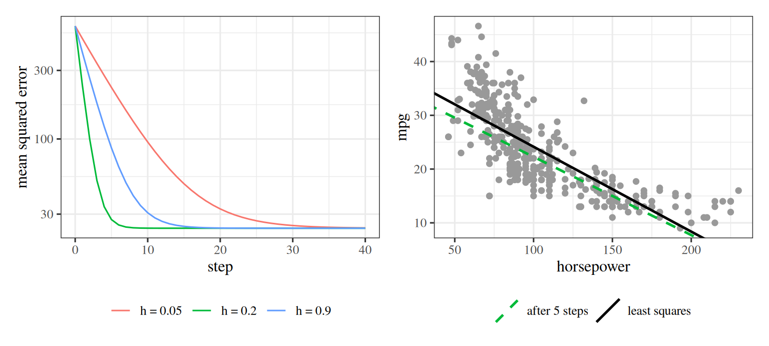
Figure 14 plots the cost against the iteration for the three step sizes of Exercise 95.
Show code
local({
  # HTML formats get an interactive plotly figure.
  # Handout and other static formats get the same curves drawn with ggplot2.
  # Load the Auto data and keep complete rows for miles per gallon and horsepower.
  auto_gd <- na.omit(read.csv("data/auto.csv")[, c("mpg", "horsepower")])
  # Standardize horsepower to mean zero and unit standard deviation.
  z_hp <- (auto_gd$horsepower - mean(auto_gd$horsepower)) / sd(auto_gd$horsepower)
  X_gd <- cbind(1, z_hp)
  y_gd <- auto_gd$mpg

  # Define the sample mean squared error and its gradient.
  cost_gd <- function(b) mean((X_gd %*% b - y_gd)^2)
  grad_gd <- function(b) drop(2 * t(X_gd) %*% (X_gd %*% b - y_gd) / length(y_gd))

  # Run gradient descent from the origin for forty iterations at three constant step sizes.
  start_b <- c(0, 0)
  step_sizes <- c(small = 0.05, middle = 0.2, large = 0.9)
  n_iter <- 40
  iters <- 0:n_iter

  run_descent <- function(h) {
    b <- start_b
    losses <- numeric(n_iter + 1)
    losses[1] <- cost_gd(b)
    for (t in seq_len(n_iter)) {
      b <- b - h * grad_gd(b)
      losses[t + 1] <- cost_gd(b)
    }
    losses
  }
  loss_histories <- lapply(step_sizes, run_descent)

  # Compute the exact least-squares minimum cost for the horizontal reference line.
  min_cost <- cost_gd(coef(lm(y_gd ~ z_hp)))

  labels <- paste0("step size: ", step_sizes)
  names(labels) <- names(step_sizes)
  colors <- c(small = "#1f77b4", middle = "#2ca02c", large = "#d95f02")

  if (knitr::is_html_output()) {
    library(plotly)

    widget <- plot_ly()
    for (nm in names(loss_histories)) {
      widget <- widget |>
        add_trace(
          x = iters,
          y = loss_histories[[nm]],
          type = "scatter",
          mode = "lines+markers",
          name = labels[[nm]],
          line = list(color = colors[[nm]]),
          marker = list(color = colors[[nm]], size = 5),
          hovertemplate = "iteration %{x}<br>sample mean squared error %{y:.2f}<extra></extra>"
        )
    }
    widget <- widget |>
      add_trace(
        x = c(0, n_iter),
        y = c(min_cost, min_cost),
        type = "scatter",
        mode = "lines",
        name = "least-squares minimum",
        line = list(color = "#888888", dash = "dash", width = 1.5),
        hovertemplate = "least-squares minimum %{y:.2f}<extra></extra>"
      ) |>
      layout(
        xaxis = list(
          title = "iteration",
          zeroline = FALSE
        ),
        yaxis = list(
          title = "sample mean squared error (mpg squared)",
          type = "log",
          zeroline = FALSE
        ),
        legend = list(orientation = "h", x = 0.5, xanchor = "center", y = -0.2),
        margin = list(t = 10, b = 90)
      ) |>
      config(displaylogo = FALSE, responsive = TRUE)

    # Attach accessible alt text because a plotly widget has none of its own.
    htmltools::div(
      role = "img",
      `aria-label` = paste(
        "Interactive logarithmic-scale plot of sample mean squared error versus iteration",
        "for gradient descent on the Auto data with three step sizes:",
        "step size 0.05 decays slowly,",
        "step size 0.2 converges quickly to the dashed least-squares minimum line,",
        "and step size 0.9 converges more slowly due to overshooting."
      ),
      widget
    )
  } else {
    library(ggplot2)

    curve_df <- do.call(
      rbind,
      lapply(names(loss_histories), function(nm) {
        data.frame(
          iteration = iters,
          loss = loss_histories[[nm]],
          step = labels[[nm]]
        )
      })
    )
    curve_df$step <- factor(curve_df$step, levels = unname(labels))

    ggplot(curve_df, aes(x = iteration, y = loss, colour = step)) +
      geom_hline(
        yintercept = min_cost,
        linetype = "dashed",
        colour = "grey40",
        linewidth = 0.5
      ) +
      geom_line() +
      geom_point(size = 1.2) +
      scale_y_log10() +
      scale_colour_manual(values = setNames(unname(colors), unname(labels))) +
      labs(
        x = "iteration",
        y = "sample mean squared error (mpg squared)",
        colour = NULL
      ) +
      theme(
        legend.position = "bottom"
      )
  }
})15 Where this goes next
Gradient descent, or a variant of it, fits many of the models in the rest of these notes. Three topics continue this chapter directly:
Logistic Regression is where these notes first take these steps on a model with no closed form. Its gradient, \(\sum_i (\sigmoid(\dprod{\vcoef}{\vx_i}) - y_i)\vx_i\), has a shape worth comparing with the least-squares gradient: a badly wrong prediction contributes at most \(\norm{\vx_i}\) to it, where squared error contributes without bound. See Logistic Regression.
-
Neural networks are fitted by exactly the algorithm on this page, with two additions. Backpropagation is how \(\grad C\) is computed when the model is a composition of many layers, and the cost is no longer convex, so the guarantees of Exercise 24 do not apply — there are many local minima, and which one we reach depends on \(\vcoef_0\). See Neural Networks.
Watch
Sanderson shows gradient descent training a neural network, from 6:55 [25, Ch. 2].
The modern optimizers — momentum, AdaGrad, RMSProp, Adam, built in Momentum and adaptive step sizes — are all modifications of the update rule in The algorithm, and all of them are attempts to reduce the effect of the condition-number problem of Exercise 33 without computing any eigenvalues. Momentum adds a fraction of the previous step to the current one, which damps the zig-zag; the adaptive methods give each coordinate its own step size, which is an inexpensive substitute for rescaling the features.
16 Further reading
Boyd and Vandenberghe [26], Section 9.3, on the gradient method and its convergence
Goodfellow et al. [19], Section 4.3
Zhou [27] and Zhou [28] — Biostat M257 slides on Newton steps, quasi-Newton methods (BFGS and limited-memory BFGS), and Fisher scoring; the Optimization page of the math notes develops the optimization methods with proofs
Robbins and Monro [13] — the stochastic approximation method that stochastic gradient descent descends from
Starmer [29], on gradient descent — an illustrated walk-through with little algebra