---
title: "Chapter 10: Nonconjugate priors and Metropolis-Hastings algorithms"
author: "Jesse Mu"
date: "December 8, 2016"
format:
html: default
revealjs:
output-file: 10-slides.html
pdf:
output-file: 10-handout.pdf
docx:
output-file: 10-handout.docx
---
<!-- Setup -->
```{r echo=FALSE, message=FALSE}
knitr::opts_chunk$set(fig.align = 'center', message = FALSE)
library(knitr)
library(ggplot2)
library(cowplot)
library(tidyr)
library(dplyr)
```
<!-- Begin writing -->
# Generalized linear models
Poisson + logistic. No conjugate priors.
# Metropolis algorithm
<!--
$$
\begin{aligned}
r &= \frac{p(\theta^* \mid y)}{p(\theta)^{(s)} \mid y} \\
&= p(\theta^* \mid y) \frac{1}{p(\theta^{(s)} \mid y)} \\
\end{aligned}
$$
TODO expand. also might include the J ratio (that's why it has to be symmetric)
-->
```{r}
s2 = 1; t2 = 10; mu = 5
y = c(9.37, 10.18, 9.16, 11.60, 10.33)
theta = 0
delta2 = 2
S = 10000
THETA = rep(NA, S)

set.seed(1)

# theta - current sample
# theta.star - proposed sample according to proposal distribution
# log.r - acceptance ratio
for (s in 1:S) {
  theta.star = rnorm(1, theta, sqrt(delta2))
  log.r = (sum(dnorm(y, theta.star, sqrt(s2), log = TRUE)) +
             dnorm(theta.star, mu, sqrt(t2), log = TRUE)) -
    (sum(dnorm(y, theta, sqrt(s2), log = TRUE)) +
       dnorm(theta, mu, sqrt(t2), log = TRUE))

  if (log(runif(1)) < log.r) theta = theta.star

  THETA[s] = theta
}
```
```{r}
theta.df = data.frame(
  iteration = 1:S,
  theta = THETA
)
ggplot(theta.df, aes(x = iteration, y = theta)) +
  geom_line()
```
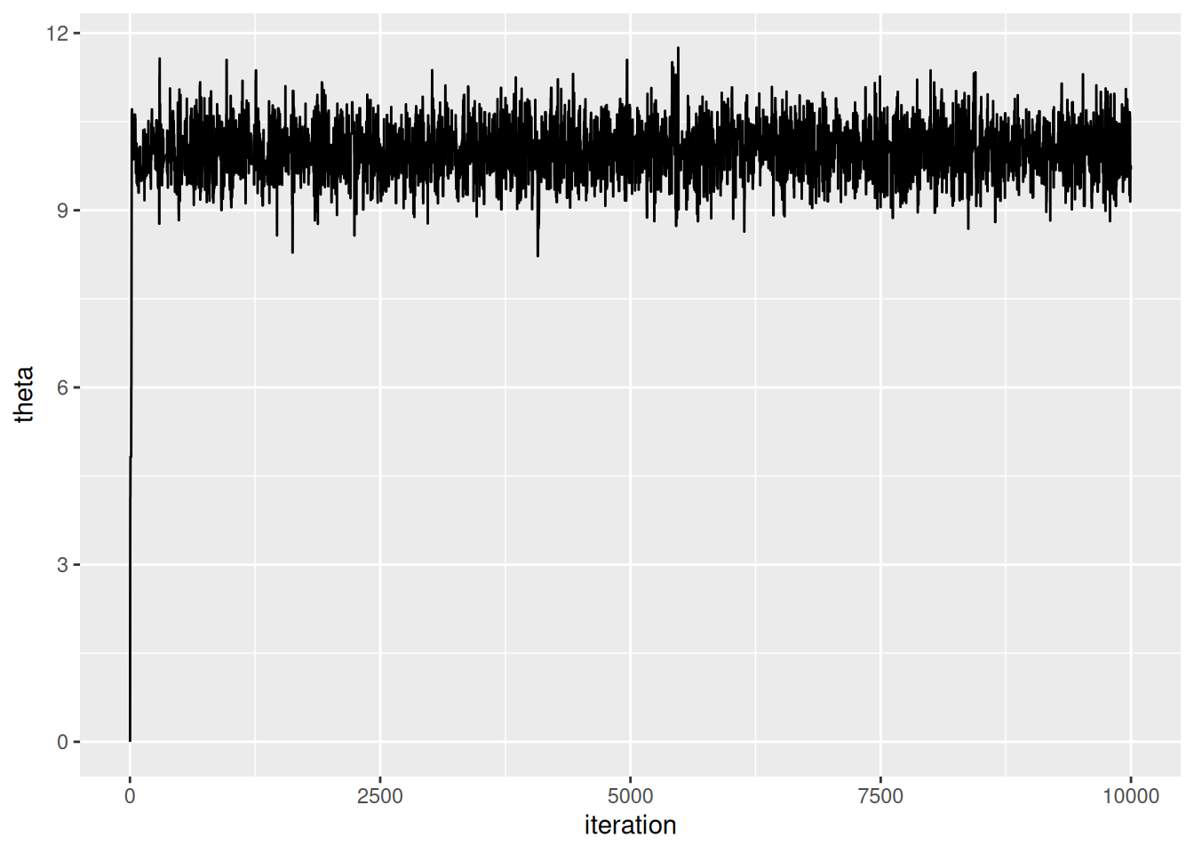
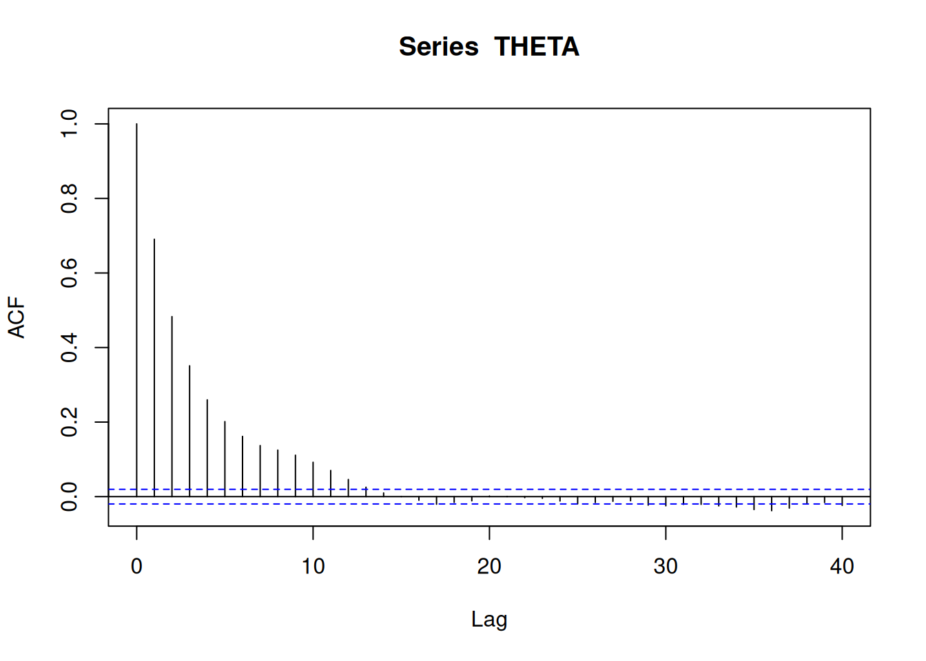
Interestingly, the effective sample sizes is quite low, only in the low thousands:
```{r}
library(coda)
effectiveSize(THETA)
```
```{r}
acf(THETA)
```
```{r}
real.df = data.frame(
  theta = seq(8, 12, length = 500),
  density = dnorm(seq(8, 12, length = 500), 10.03, .44)
)
ggplot(theta.df) +
  geom_histogram(aes(x = theta, y = ..density..), bins = 60) +
  geom_line(data = real.df, mapping = aes(x = theta, y = density))
# outs[, 4]
# distribution looks different if we include 25000 vs ...  1000
```
### Output of the Metropolis algorithm
Need to run until stationarity
Different proposal distributions. Delta as a tradeoff between rate of approach towards the HPD region versus overshooting (like learning rate in gradient descent, etc)
Acceptance rate of between 20 and 50% is good. Control length
## Combining Metropolis and Gibbs algorithms
Since proposal distributions for different parameters can all be different -
could use Gibbs for some parameters (where Gibbs is just a special case of
Metropolis-Hastings)
### A regression model with correlated errors
This section explores running multiple independent MCMC chains and
combining the data (which is theoretically OK). The approach in `icecore_parallel.R` is to take
the MH algorithm for analyzing the icecore data and distribute it across
multiple cores with `parallel::mclapply`. That file creates `icecore_mcmc` which
is analyzed here.
```{r}
if (!file.exists('./icecore_mcmc')) {
  stop("Run icecore_parallel.R first to get MCMC data")
}
load('./icecore_mcmc')
# Should have "outs" now
# TODO: put colnames in icecore_parallel
colnames(outs) = c('b1', 'b2', 's2', 'phi')
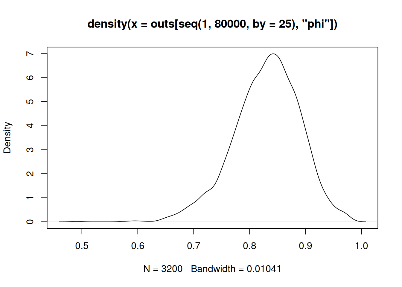
plot(density(outs[seq(1, 80000), 'phi']))
plot(density(outs[seq(1, 80000, by = 25), 'phi']))
outs.df = data.frame(outs)
outs.df$iteration = 1:nrow(outs.df)

message(nrow(outs.df), " samples in ./icecore_mcmc")

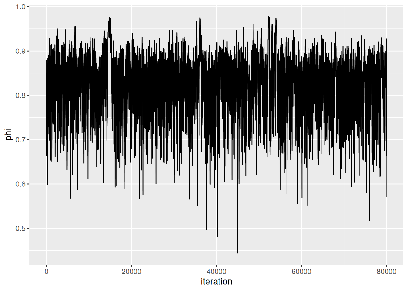
ggplot(outs.df, aes(x = iteration, y = phi)) +
  geom_line()
effectiveSize(outs.df$phi)
```
# Exercises
<!--
## 10.1
When $\theta_0 > \delta$, $\tilde{\theta} \in [\theta_0 - \delta, \theta_0 + \delta] > 0$, so $\theta_1 \sim \text{uniform}(\theta_0 - \delta, \theta_0 + \delta)$ and
$$
J(\theta_1 \mid \theta_0) = \frac{1}{2\delta}
$$
-->
## 10.2
```{r}
msparrownest = read.table('Exercises/msparrownest.dat')
```
For convenience let $\theta_i = P(Y_i = 1 \mid \alpha, \beta, x_i)$. Now we solve for $\theta_i$ in our model
$$
\begin{aligned}
& \log\left(\frac{\theta_i}{1 - \theta_i}\right) = \alpha + \beta x_i \\
\implies& \frac{\theta_i}{1 - \theta_i} = \exp(\alpha + \beta x_i) \\
\implies& \theta_i = \exp(\alpha + \beta x_i) - \theta_i \exp(\alpha + \beta x_i) \\
\implies& \theta_i = \frac{\exp(a + \beta x_i)}{1 + \exp(\alpha + \beta x_i)}
\end{aligned}
$$
So we know $Y_i \sim \text{Bernoulli}\left(p_i\right)$ where $p_i = \frac{\exp(a + \beta x_i)}{1 + \exp(a + \beta x_i)}$ and thus
$$
p(y_i \mid \alpha, \beta, x_i) = p_i^{y_i}(1 - p_i)^{1 - y_i}
$$
### a
Let $z_i = \exp(\alpha + \beta x_i)$ for simplicity.
$$
\begin{aligned}
p(\boldsymbol{y} \mid \alpha, \beta, x_i) &= \prod_{i = 1}^n p(y_i \mid \alpha, \beta, x_i) \\
&= \prod_{i = 1}^n p_i^{y_i} (1 - p_i)^{1 - y_i} \\
&= \prod_{i = 1}^n \left(\frac{z_i}{1 + z_i} \right)^{y_i} \left(1 - \frac{z_i}{1 + z_i} \right)^{1 - y_i} \\
&= \prod_{i = 1}^n \left(\frac{z_i}{1 + z_i} \right)^{y_i} \left(\frac{1 + z_i}{1 + z_i} - \frac{z_i}{1 + z_i} \right)^{1 - y_i} \\
&= \prod_{i = 1}^n \left(\frac{z_i}{1 + z_i} \right)^{y_i} \left(\frac{1}{1 + z_i}\right)^{1 - y_i} \\
&= \prod_{i = 1}^n \frac{z_i^{y_i}}{(1 + z_i)^{y_i}} \frac{1}{(1 + z_i)^{1 - y_i}} \\
&= \prod_{i = 1}^n \frac{z_i^{y_i}}{1 + z_i} \\
&= \prod_{i = 1}^n \frac{\exp(y_i (\alpha + \beta x_i))}{1 + \exp(\alpha + \beta x_i)} \\
\end{aligned}
$$
and this cannot be simplified further.
### b
It's helpful to think about this in terms of the log-odds, i.e.,
$\text{log-odds}(\theta_i) = a + \beta x_i$. With an uninformative prior
where no interaction between wingspan $x_i$ and nesting is assumed by default,
the prior for $\beta$ should be centered around 0. To also be
uninformative about the prior proportion of nesting birds regardless of
wingspan, the prior for $\alpha$ should be centered around 0 as well, so the
prior expectation regardless of $x_i$ is $\text{log-odds}(\theta_i) = 0 + 0 x_i = 0$ (thus not favoring nesting or not).
The question is what to use for a prior distribution and how diffuse to make the
priors. Priors for $\alpha$ and $\beta$ should be symmetric, so normal
distributions for both make sense. For an uninformative prior,
the variance of these normals should be set high.
If $\alpha$ is always 0, then as $x$ moves from 10 to 15, the possible
values of $\beta$ should allow for a change in the log-odds ratio from approximately
0 to 1. Note the log-odds ratio of some sufficiently small number e.g. `1e-5`
is `r log(1e-5 / (1 - 1e-5))` which is roughly 10. Since $x$ at a minimum is 10,
it makes sense to have most of the prior on $\beta$ in the range $[-10 / 10, 10 / 10] = [-1, 1]$,
so the standard deviation of the $\beta$ prior is set to 0.5
and the variance to 0.25.
Similarly, the standard deviation of the
$\alpha$ prior to be 5 and the variance 25, so that, if $\beta = 0$, the most of
the $\alpha$ prior falls in the log-odds interval $[-10, 10]$.
So
$$
\begin{aligned}
\alpha &\sim \mathcal{N}(0, 25) \\
\beta &\sim \mathcal{N}(0, 0.25) \\
\end{aligned}
$$
### c
```{r}
library(MASS)
inv = solve
# In this sampling scheme, when we sample, we keep the values together
# ($\theta$). But when I store the values, I split them (ALPHA, BETA).
S = 10000
burnin = 5000
y = msparrownest[, 1]
n = length(y)
# Use linear regression format, where column 1 is 1 (for alpha) and column 2 is
# the wingspan
x = cbind(rep(1, n), msparrownest[, 2])
# Start with X^T X but increase until acceptance ratio between 30% - 50%
var.prop = 7 * inv(t(x) %*% x)
# Prior parameters
pmn.theta = c(0, 0)
psd.theta = sqrt(c(25, 0.25))
# Where to store values
ALPHA = numeric(S + burnin)
BETA = numeric(S + burnin)
# Acceptances
acs = 0
# Initial estimates
theta = c(0, 0)
# For calculating likelihood ratio
log.p.y = function(x, y, theta) {
exp_term = exp(x %*% theta)
p = exp_term / (1 + exp_term)
sum(dbinom(y, 1, p, log = TRUE))
}
p.theta = function(theta) {
sum(dnorm(theta, pmn.theta, psd.theta, log = TRUE))
}
for (s in 1:(S + burnin)) {
theta.star = mvrnorm(1, theta, var.prop)
lhr = log.p.y(x, y, theta.star) +
p.theta(theta.star) -
log.p.y(x, y, theta) -
p.theta(theta)
if (log(runif(1)) < lhr) {
theta = theta.star
if (s > burnin) {
acs = acs + 1
}
}
ALPHA[s] = theta[1]
BETA[s] = theta[2]
}
ALPHA = ALPHA[burnin:length(ALPHA)]
BETA = BETA[burnin:length(BETA)]
message("Acceptance ratio: ", acs / S) # Good to go
c(effectiveSize(ALPHA), effectiveSize(BETA))
```
### d
```{r}
alpha_prior = data.frame(
  val = seq(-10, 10, length.out = 1000),
  density = dnorm(seq(-10, 10, length.out = 1000), 0, 5),
  var = 'alpha',
  dist = 'prior'
)
beta_prior = data.frame(
  val = seq(-1, 1, length.out = 1000),
  density = dnorm(seq(-1, 1, length.out = 1000), 0, 0.5),
  var = 'beta',
  dist = 'prior'
)
prior_df = rbind(alpha_prior, beta_prior)
alpha_post = data.frame(
  val = ALPHA,
  var = 'alpha',
  dist = 'posterior'
)
beta_post = data.frame(
  val = BETA,
  var = 'beta',
  dist = 'posterior'
)
post_df = rbind(alpha_post, beta_post)

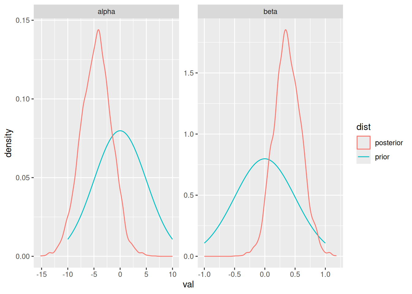
ggplot(prior_df, aes(x = val, y = density, color = dist)) +
  geom_line() +
  geom_density(data = post_df, mapping = aes(x = val, y = ..density..)) +
  facet_wrap(~ var, scales = 'free')
```
### e
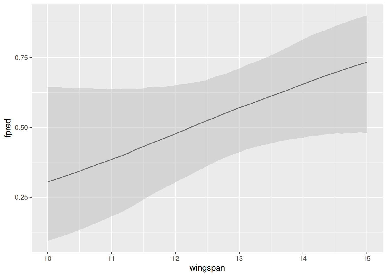
Using the samples of $\alpha$ and $\beta$, simply compute a distribution on
$f_{\alpha\beta}(x)$. Confidence intervals can then be constructed around this
distribution. However, this needs to be done for many $x$ values:
```{r}
x_seq = seq(10, 15, length = 100)
quantiles = sapply(x_seq, function(x) {
  exp_term = exp(ALPHA + BETA * x)
  fab = exp_term / (1 + exp_term)
  quantile(fab, probs = c(0.025, 0.5, 0.975))
})

fab_df = data.frame(
  wingspan = x_seq,
  ymin = quantiles[1, ],
  fpred = quantiles[2, ],
  ymax = quantiles[3, ]
)

ggplot(fab_df, aes(x = wingspan, y = fpred, ymin = ymin, ymax = ymax)) +
  geom_line() +
  geom_ribbon(fill = 'grey', alpha = 0.5)
```
This is the logistic regressions' approximate probability of nesting based on
wingspan, although the confidence intervals are quite wide.