---
title: "Chapter 8: Group comparisons and hierarchical modeling"
author: "Jesse Mu"
date: "November 17, 2016"
format:
html: default
revealjs:
output-file: 8-slides.html
pdf:
output-file: 8-handout.pdf
docx:
output-file: 8-handout.docx
---
<!-- Setup -->
```{r echo=FALSE, message=FALSE}
knitr::opts_chunk$set(fig.align = 'center', message = FALSE)
library(knitr)
library(ggplot2)
library(cowplot)
library(tidyr)
library(dplyr)
```
<!-- Begin writing -->
A common task in data analysis is to compare summary statistics for two or more
groups. In this chapter we cover the Bayesian approach to doing this.
# Comparing two groups
::: notes
A standard method in (frequentist) introductory statistics for comparing the
means of two populations is to compute the $t$-statistic of the observed mean
difference and obtain the two-sided $p$-value. Then, if $p < 0.05$ (or any other
significance level), we reject the null hypothesis that the two groups have the
same mean, and use the estimates $\hat{\theta}_1 = \bar{y}_1$ and
$\hat{\theta}_2 = \bar{y}_2$ (i.e. the ML estimators for $\theta_1$ and
$\theta_2$ independently). Otherwise, we accept the null hypothesis that the two
groups have the same mean and let $\hat{\theta}_1 = \hat{\theta}_2$ be the
pooled mean of the two groups.
There are many situations in which this paradigm doesn't make too much sense.
Consider borderline cases in which our $p$-value is close to 0.05. It seems like
a technicality to treat the means as completely different if e.g. $p = 0.051$,
and completely the same if $p = 0.049$ - a difference that could hypothetically
be observed by simply sampling one more data point.
:::
The Bayesian approach is to treat the two populations as being sampled from a
common mean $\theta$ plus some difference $\delta$, where we estimate both
$\theta$ and $\delta$. Then the observed difference $\delta$ can vary
continuously. Specifically, our sampling model for a value from either group is
- $Y_{i, 1} = \mu + \delta + \epsilon_{i, 1}$
- $Y_{i, 2} = \mu + \delta + \epsilon_{i, 2}$
where we assume values from both groups have a common variance $\epsilon_{i, j} \sim \text{i.i.d.}\; \mathcal{N}(0, \sigma^2)$.
## Prior and posterior distributions
### Prior
The joint prior for all three parameters of our model $\mu, \delta, \sigma^2$ is
unsurprising. We treat the parameters as independent, so $p(\mu, \delta, \sigma^2) = p(\mu) p(\delta) p(\sigma^2)$ where
- $\mu \sim \mathcal{N}(\mu_0, \gamma_0^2)$
- $\delta \sim \mathcal{N}(\delta_0, \tau_0^2)$
- $\sigma^2 \sim \text{inverse-gamma}(\nu_0 / 2, \sigma_0^2 \nu_0 / 2)$
Notice that we specify prior distributions for the common mean and variance, but
we also express an estimate (and certainty of the estimate) for the difference
between the group means $\delta$.
### Posterior
Then the full conditional distributions of the parameters are
- $\mu \mid \boldsymbol{y}_1, \boldsymbol{y}_2, \delta, \sigma^2 \sim \mathcal{N}(\mu_n, \gamma_n^2)$
- $\mu_n = \gamma_n^2 \times \left[ \mu_0 / \gamma_0^2 + \sum_{i = 1}^{n_1} (y_{i, 1} - \delta) / \sigma^2 + \sum_{i = 1}^{n_2}(y_{i, 2} + \delta) / \sigma^2 \right]$
- $\gamma_n^2 = \left[ 1/\gamma_0^2 + (n_1 + n_2) / \sigma^2 \right]^{-1}$
- $\delta \mid \boldsymbol{y}_1, \boldsymbol{y}_2, \mu, \sigma^2 \sim \mathcal{N}(\delta_n, \tau_n^2)$
- $\delta_n = \tau_n^2 \times \left[ \delta_0 / \tau_0^2 + \sum_{i = 1}^{n_1} (y_{i, 1} - \mu) / \sigma^2 - \sum_{i = 1}^{n_2} (y_{i, 2} - \mu) / \sigma^2 \right]$
- $\tau_n^2 = \left[ 1 / \tau_0^2 + (n_1 + n_2) / \sigma^2 \right]^{-1}$
- $\sigma^2 \mid \boldsymbol{y}_1, \boldsymbol{y}_2, \mu, \delta \sim \text{inverse-gamma}(\nu_n / 2, \sigma_n^2 \nu_n / 2)$
- $\nu_n = \nu_0 + n_1 + n_2$
- $\nu_n \sigma_n^2 = \nu_0 \sigma_0^2 + \sum_{i = 1}^{n_1} (y_{i, 1} - \left[\mu + \delta \right])^2 + \sum_{i = 1}^{n_2} (y_{i, 2} - \left[ \mu - \delta \right])^2$
## Analysis of the math score data
```{r}
source('Replication/chapter8.R')
y1 = y.school1
y2 = y.school2
n1 = length(y1)
n2 = length(y2)

# Priors
mu0 = 50
g20 = 625
del0 = 0
t20 = 625
s20 = 100
nu0 = 1

# starting values based on ML estimates
mu = (mean(y1) + mean(y2)) / 2
del = (mean(y1) - mean(y2)) / 2

# Gibbs sampler
S = 5000
MU = rep(0, S)
DEL = rep(0, S)
S2 = rep(0, S)
Y12 = matrix(0, nrow = S, ncol = 2)

set.seed(1)
for (s in 1:S)  {

  # Sample s2 according to p.128 eq 3
  s2 = 1 / rgamma(1, (nu0 + n1 + n2) / 2,
                  (nu0 * s20 + sum((y1 - mu - del)^2) + sum((y2 - mu + del)^2)) / 2)

  # Sample mu according to p.128 eq 1
  var.mu = 1 / (1 / g20 + (n1 + n2) / s2)
  mean.mu = var.mu * (mu0/g20 + sum(y1 - del) / s2 + sum(y2 + del) / s2)
  mu = rnorm(1, mean.mu, sqrt(var.mu))

  # Sample del according to p.128 eq 2
  var.del = 1 / (1 / t20 + (n1 + n2) / s2 )
  mean.del = var.del * (del0 / t20 + sum(y1 - mu) / s2 - sum(y2 - mu) / s2)
  del = rnorm(1, mean.del, sqrt(var.del))

  # Store params
  MU[s] = mu
  DEL[s] = del
  S2[s] = s2
  # Sample from posterior
  Y12[s, ] = rnorm(2, mu + c(1, -1) * del, sqrt(s2))
}

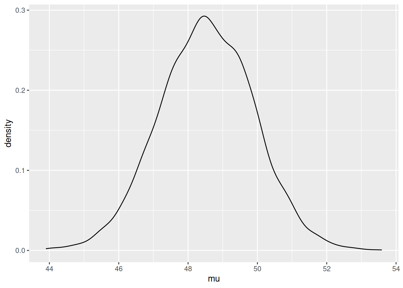
ggplot(data.frame(mu = MU)) +
  geom_density(aes(x = mu))
```
Now we can directly estimate the probability that $\delta > 0$:
```{r}
mean(DEL > 0)
```
as well as the probability that an individual from school 1 is higher than school 2, which due to variance is a bit lower:
```{r}
mean(Y12[, 1] > Y12[, 2])
```
# Comparing multiple groups
---
Let's extend this to a $> 2$ group case. Assume for our example above that we
have many schools, which we assume are samples from a population of schools. So
our dataset is *hierarchical* or *multilevel* since there are samples of schools
and within each school samples of students.
## Exchangeability and hierarchical models
Using de Finetti's theorem and assuming exchangability, we knew previously that
for a single group, we can treat the data within the group as being
conditionally i.i.d. given a parameter, which we call the **within-group sampling variability**:
$$
\{Y_{1, j}, \dots, Y_{n_{j}, j} \mid \phi_j\} \sim \text{i.i.d.}\; p(y \mid \phi_j)
$$
Further, if we have many groups with parameters $\phi_j$ that we assume are
sampled from a population of *groups* we can again use de Finetti's theorem to
treat the group means $\phi_j$ as conditionally i.i.d. given another parameter,
which we call the **between-group sampling variability**:
$$
\{\phi_{1}, \dots, \phi_{m} \mid \psi\} \sim \text{i.i.d.} \; p(\phi \mid \psi)
$$
Then we simply need a prior distribution on the parameter for the group parameters (a "hyperparameter") $\psi$:
$$
\psi \sim p(\psi)
$$
Note that we can extend this hierarchy arbitrarily.
# The hierarchical normal model
---
The key of the hierarchical normal model is to treat the data within a group as
being normally distributed with some mean $\theta_j$ and variance $\sigma^2$, and the means among
groups to *also* be normally distributed according to some other mean $\mu$ and
variance $\tau^2$. Note that for now we're assuming that the data within groups share a
common variance $\sigma^2$ that doesn't depend on the group $j$.
Specifically, we have
- $Y_{i, j} \sim \mathcal{N}(\theta_j, \sigma^2)$
- $\theta_j \sim \mathcal{N}(\mu, \tau^2)$
So for $m$ groups, we have unknown parameters $\{\theta_1, \dots, \theta_m\}$,
the within-group variance $\sigma^2$, and the mean and variance of the group
means $(\mu, \tau^2)$. Notice that there are three fixed parameters for which we
need to specify prior distributions: $\mu$, $\tau^2$, and $\sigma^2$. Our priors
will be standard inverse-gamma and normal semiconjugate priors:
\begin{align}
\sigma^2 &\sim \text{inverse-gamma}(\nu_0 / 2, \sigma_0^2 \nu_0 / 2) \\
\tau^2 &\sim \text{inverse-gamma}(\eta_0 / 2, \tau_0^2 \eta_0 / 2) \\
\mu^2 &\sim \mathcal{N}(\mu_0, \gamma_0^2)
\end{align}
**Fig 8.3** isn't reproduced here in these notes but is important for
visualizing the model. It especially helps to know how Bayesian networks are interpreted,
which helps explain the conditional dependencies.
## Posterior inference
### Intuition
We have samples from $m$ groups $\{\boldsymbol{y}_1, \dots, \boldsymbol{y}_m\}$. Our task is to sample from the posterior distribution
$$
p(\theta_1, \dots, \theta_m, \mu, \tau^2, \sigma^2 \mid \boldsymbol{y}_1, \dots, \boldsymbol{y}_m)
$$
for which we'll use a Gibbs sampler. We need to find the full conditionals for
all unknown quantities above, which seems intimidating. In the Chapter 6 notes
In the Chapter 6 notes ("a shortcut for thinking about full conditionals"), it should be mentioned that
obtaining the full conditional for a single parameter is fairly straightforward
by simply writing the entire joint posterior but then treating the other
parameters as constants that can be discarded via proportionality.
To obtain the full joint posterior we will take use key independence assumptions
between the parameters of our model. For example, given a group-specific mean
$\theta_j$, the corresponding random variables $Y_{i, j}$ depend only on
$(\theta_j, \sigma^2)$ and not on $\mu$ or $\tau^2$ (this is implied in Figure
8.3).
\begin{align}
& p(\theta_1, \dots, \theta_m, \mu, \tau^2, \sigma^2 \mid \boldsymbol{y}_1, \dots, \boldsymbol{y}_m) \\
\quad&\propto p(\mu, \tau^2, \sigma^2, \mu, \tau^2, \sigma^2) \times p(\boldsymbol{y}_1, \dots, \boldsymbol{y}_m \mid \theta_1, \dots, \theta_m, \mu, \tau^2, \sigma^2) & \text{Bayes' rule} \\
&= p(\mu, \tau^2, \sigma^2) \times p(\theta_1, \dots, \theta_m \mid \mu, \tau^2, \sigma^2) \times p(\boldsymbol{y}_1, \dots, \boldsymbol{y}_m \mid \theta_1, \dots, \theta_m, \mu, \tau^2, \sigma^2) & \text{Chain rule} \\
&= p(\mu) p(\tau^2) p(\sigma^2) \times p(\theta_1, \dots, \theta_m \mid \mu, \tau^2) \times p(\boldsymbol{y}_1, \dots, \boldsymbol{y}_m \mid \theta_1, \dots, \theta_m, \sigma^2) & \text{Indep.} \\
&= p(\mu) p(\tau^2) p(\sigma^2) \times \left[ \prod_{j = 1}^m p(\theta_j \mid \mu, \tau^2) \right] \times \left[ \prod_{j = 1}^m p(\boldsymbol{y}_j \mid \theta_j, \sigma^2) \right] & \text{de Finetti} \\
&= p(\mu) p(\tau^2) p(\sigma^2) \times \left[ \prod_{j = 1}^m p(\theta_j \mid \mu, \tau^2) \right] \times \left[ \prod_{j = 1}^m \left( \prod_{i = 1}^{n_j} p(y_{i, j} \mid \theta_j, \sigma^2) \right) \right] & \text{de Finetti 2x} \\
\end{align}
Now to evaluate a full conditional, for example that for $\mu$, we take the full posterior and discard all terms that don't depend on $\mu$:
$$p(\mu \mid \theta_1, \dots, \theta_m, \tau^2, \sigma^2, \boldsymbol{y}_1, \dots, \boldsymbol{y}_m) \propto p(\mu) \prod_{j=1}^m p(\theta_j \mid \mu, \tau^2)$$
which in this case looks exactly like a standard one-sample Normal posterior
from Chapter 6, so we borrow that result and replace the relevant variables from
our priors. We can do this similarly for the other parameters.
### Quantities
Since the work is quite tedious, the derivations for the full
conditionals of the parameters. To summarize, given priors
\begin{align}
\sigma^2 &\sim \text{inverse-gamma}(\nu_0 / 2, \sigma_0^2 \nu_0 / 2) \\
\tau^2 &\sim \text{inverse-gamma}(\eta_0 / 2, \tau_0^2 \eta_0 / 2) \\
\mu^2 &\sim \mathcal{N}(\mu_0, \gamma_0^2)
\end{align}
the full conditionals are
\begin{align}
\{\mu \mid \theta_1, \dots, \theta_m, \tau^2\} &\sim \mathcal{N}\left(\frac{m\bar{\theta} / \tau^2 + \mu_0 / \gamma_0^2}{m/\tau^2 + 1 / \gamma_0^2}, \left[m / \tau^2 + 1 / \gamma_0^2 \right]^{-1}\right) \\
\{\tau^2 \mid \theta_1, \dots, \theta_m, \mu\} &\sim \text{inverse-gamma}\left(\frac{\eta_0 + m}{2}, \frac{\eta_0\tau_0^2 + \sum_{j = 1}^{m}(\theta_j - \mu)^2}{2} \right) \\
\{\theta_j \mid y_{1, j}, \dots, y_{n_{j}, j}, \sigma^2\} &\sim \mathcal{N}\left(\frac{n_j\bar{y}_j / \sigma^2 + 1 / \tau^2}{n_j / \sigma^2 + 1 / \tau^2}, \left[ n_j / \sigma^2 + 1 / \tau^2 \right]^{-1} \right) \\
\{\sigma^2 \mid \boldsymbol{\theta}, \boldsymbol{y_1}, \dots, \boldsymbol{y_n}\} &\sim \text{inverse-gamma}\left(\frac{1}{2}\left[ \nu_0 + \sum_{j = 1}^m n_j\right], \frac{1}{2}\left[\nu_0\sigma_0^2 + \sum_{j = 1}^{m} \left( \sum_{i = 1}^{n_j} (y_{i, j} - \theta)^2 \right) \right] \right)
\end{align}
It's worth briefly discussing what these values represent. The full conditionals
for $\mu$ and $\tau^2$ look like standard normal posteriors. Similarly, the full
conditional for $\theta_j$ looks like a normal posterior dependent only on the
specific subgroup $\boldsymbol{y}_j$ and the common variance $\sigma^2$. Lastly
(and most interestingly), notice that the posterior for $\sigma^2$ looks like a
standard inverse gamma posterior which depends on $\sum \sum (y_{i, j} -
\theta)^2$ which is the pooled variance across all groups (see also $\sum n_j$).
# Example: Math scores in U.S. public schools
---
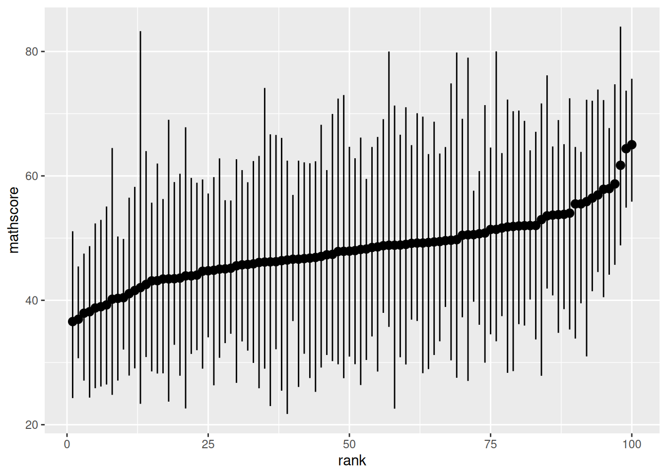
We now look at the full dataset of math scores from 100 schools:
```{r echo=FALSE}
library(dplyr)
school.df = Y.school.mathscore %>% as.data.frame %>% tbl_df
meanscore = school.df %>%
group_by(school) %>%
summarise(meanscore = mean(mathscore)) %>%
mutate(rank = rank(meanscore))
school.toplot = school.df %>%
left_join(meanscore, by = 'school') %>%
mutate(minscore = min(mathscore), maxscore = max(mathscore))
ggplot(school.toplot, aes(x = rank, y = mathscore, group = school)) +
stat_summary(fun.ymin = min, fun.ymax = max, fun.y = mean)
```
## Prior distributions and posterior approximation
We need to specify the following priors:
$$
\sigma^2 \sim \text{inverse-gamma}(\nu_0 / 2, \sigma_0^2 \nu_0 / 2)
$$
If we know the math exam was designed to give a nationwide variance of 100, we
can set the within-school variance to 100. This is probably an overestimate
since the within-school variance should be less than the nationwide estimate.
Regardless, we set $\sigma_0^2 = 100, \nu_0 = 1$ to weakly concentrate the prior
around 100.
$$
\tau^2 \sim \text{inverse-gamma}(\eta_0 / 2, \tau_0^2 \eta_0 / 2)
$$
Similarly, we set $\tau_0^2 = 100, \eta_0 = 1$.
$$
\mu^2 \sim \mathcal{N}(\mu_0, \gamma_0^2)
$$
Since the mean over all schools should be 50, we set $\mu_0 = 50, \gamma_0^2 = 25$, so that 95% of the probability of our prior is in $(40, 60)$.
### Gibbs sampling
Now that we're sampling more and more parameters $\{\mu^{(s)}, \tau^{2(s)},
\sigma^{2(s)}, \theta_1^{(s)}, \dots, \theta_m^{(s)} \}$, there's a key point
about Gibbs sampling that must be emphasized: the order in which we sample the
new parameters doesn't matter, but each parameter must be updated according to
the *most current* values of the other parameters. That is, if we have sampled
$\mu^{(s+1)}$, the sample of $\tau^{(s + 1)}$ must be dependent on
$\mu^{(s+1)}$, **NOT** $\mu^{(s)}$. This ensures the markov chain property.
```{r}
Y = Y.school.mathscore

# Priors
nu0 = eta0 = 1
s20 = t20 = 100
mu0 = 50
g20 = 25

# Number of schools. Y[, 1] are school ids
m = length(unique(Y[, 1]))

# Starting values - use sample mean and variance
n = sv = ybar = rep(NA, m)
for (j in 1:m) {
  Y_j = Y[Y[, 1] == j, 2]
  ybar[j] = mean(Y_j)
  sv[j] = var(Y_j)
  n[j] = length(Y_j)
}
# Let initial theta estimates be the sample means
# Similarly, let initial values of sigma2, mu, and tau2 be "sample mean and
# variance"
theta = ybar
sigma2 = mean(sv)
mu = mean(theta)
tau2 = var(theta)

# MCMC
set.seed(1)
S = 1000
THETA = matrix(nrow = S, ncol = m)
# Storing sigma, mu, theta together
SMT = matrix(nrow = S, ncol = 3)

for (s in 1:S) {
  # Sample thetas
  for (j in 1:m) {
    vtheta = 1 / (n[j] / sigma2 + 1 / tau2)
    etheta = vtheta * (ybar[j] * n[j] / sigma2 + mu / tau2)
    theta[j] = rnorm(1, etheta, sqrt(vtheta))
  }

  # Sample sigma2
  nun = nu0 + sum(n) # TODO: Could cache this
  ss = nu0 * s20
  # Pool variance
  for (j in 1:m) {
    ss = ss + sum((Y[Y[, 1] == j, 2] - theta[j])^2)
  }
  sigma2 = 1 / rgamma(1, nun / 2, ss / 2)

  # Sample mu
  vmu = 1 / (m / tau2 + 1 /g20)
  emu = vmu * (m * mean(theta) / tau2 + mu0 / g20)
  mu = rnorm(1, emu, sqrt(vmu))

  # Sample tau2
  etam = eta0 + m
  ss = eta0 * t20 + sum((theta - mu)^2)
  tau2 = 1 / rgamma(1, etam / 2, ss / 2)

  # Store params
  THETA[s, ] = theta
  SMT[s, ] = c(sigma2, mu, tau2)
}
```
### MCMC diagnostics
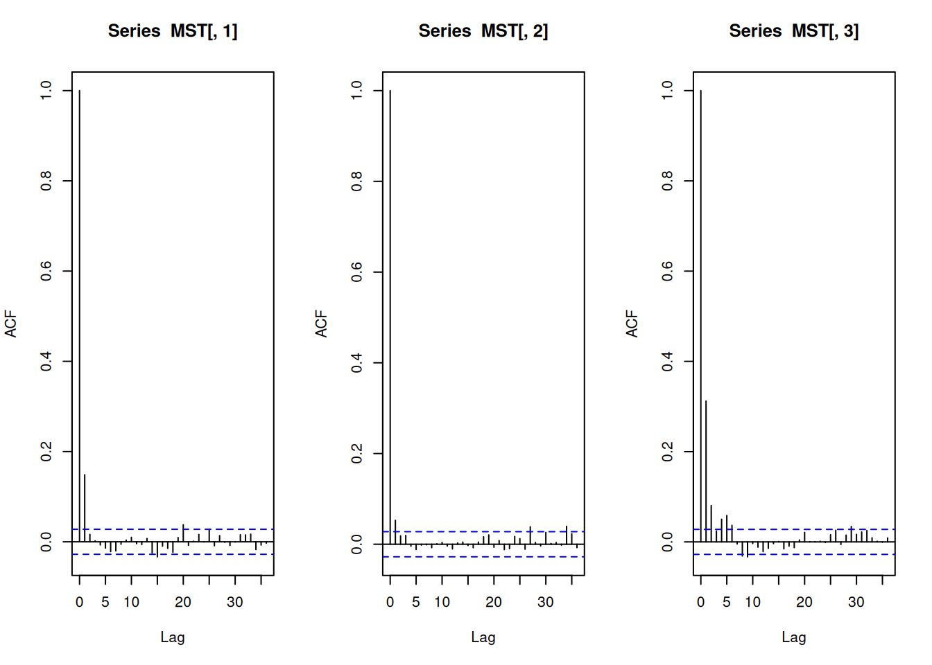
The book mentions here that it's important to check convergence of the Gibbs
sampler; this is not done here, but dividing the samples into groups of e.g. 500
samples, and ensuring that the mean values of the parameters don't change too
much from group to group is a good way to check, at least for a manageable
number of parameters.
## Posterior summaries and shrinkage
Notice from the full conditional of $\theta_j$ above that the expected value of $\theta_j$ is a weighted average of $\bar{y}_j$ and $\mu$:
\begin{align}
\mathbb{E}(\theta_j \mid \boldsymbol{y}_j, \mu, \tau^2, \sigma^2) &= \frac{\bar{y}_j n_j / \sigma^2 + \mu/\tau^2}{n_j / \sigma^2 + 1 / \tau^2} \\
&= \frac{n_j / \sigma^2}{n_j / \sigma^2 + 1 / \tau^2} \bar{y}_j + \frac{1 / \tau^2}{n_j / \sigma^2 + 1 / \tau^2} \mu
\end{align}
which is specifically weighted by the sample size $n_j$. Since we assume that
there is some common mean $\mu$, our estimate of $\theta_j$ gets pulled slightly
towards that common parameter $\mu$ - less so for high $n_j$. This demonstrates
the phonemonon of *shrinkage*, where information is shared across groups in this
hierarchical model.
Again, for high $n_j$, however, the effect of this shrinkage is neglegible.
Shrinkage results in some interesting phenomena. For example, look at schools 82
and 46 in our dataset.
```{r echo}
mean(THETA[, 82])
mean(THETA[, 46])
ybar[82]
ybar[46]
```
::: notes
Even though the sample mean of school 82 is lower than school 46, the posterior
expectation of $\theta_{82}$ is *higher* than $\theta_{46}$, because school 82 has a
very small sample and thus is affected more by a pull towards $\mu$. While this
may seem counterintuitive, the explanation is that there is more evidence that
$\theta_{46}$ is low than there is $\theta_{82}$ is low due to the wide
discrepancy in sample sizes. The assumption that $\theta_j$ stem from one $\mu$,
then, takes a "conservative" approach to estimating the $\theta_{82}$ with
little data.
:::
# Hierarchical modeling of means and variances
::: notes
The previous model assumed common variance within groups $\sigma^2$. This is
actually fairly common, perhaps less because of empirical justification for
assuming common within-group variance than lack of interest in the variance of
the groups. But of course, the inaccuracy of this assumption could result in
errors in analysis. It's fairly straightforward to simply add another
hierarchical layer for the variance too, and jointly estimate the group-specific
means and variances, as well as the common mean and variance parameters.
:::
To implement this, we let $\theta_j$ depend on $\boldsymbol{y}_j$ and (new!) a
group $j$-specific $\sigma_j^2$, so our full conditional distribution is
$$
\theta_j \mid \boldsymbol{y}_j, \sigma_j^2 \sim \mathcal{N}\left( \frac{n_j\bar{y}_j / \sigma_j^2 + 1 / \tau^2}{n_j / \sigma_j^2 + 1 / \tau^2}, \left[n_j / \sigma_j^2 + 1 / \tau^2 \right]^{-1} \right)
$$
similarly, above we had a rather special case of the full conditional of
$\sigma^2$. Since there was one common $\sigma^2$, the posterior was based on a
combination of the prior precision and the pooled sample variance. Now let's
assume that we have a separate $\sigma_j^2$ for each group:
$$\sigma_1^2, \dots, \sigma_m^2 \sim \text{i.i.d.} \; \mathcal{N}(\nu_0 / 2, \sigma_0^2 \nu_0 / 2).$$
Now that we're including individual $\sigma_j^2$, re-deriving the full
conditional for $\sigma_j^2$ results in full conditional distributions that look
just like the one-parameter case for variance (and the corresponding $\theta_j$ conditionals for the means):
$$
\sigma_j^2 \mid \boldsymbol{y}_j, \theta_j \sim \text{inverse-gamma}\left([\nu_0 - n_j] / 2, \left[\nu_0 \sigma_0^2 + \sum_{i = 1}^{n_j}(y_{i, j} - \theta_j)^2 \right] / 2 \right)
$$
Now in the same way that we learn the group-specific parameters $\mu, \tau^2$
using prior distributions with hyperparameters $\eta_0, \tau_0^2, \mu_0,
\gamma_0^2$, we should learn $\nu_0, \sigma_0^2$ with prior distributions.
Since we are modeling variances, we let $\sigma_0^2 \sim \text{gamma}(a, b)$ such that the posterior is
$$
\sigma_0^2 \mid \sigma_1^2, \dots, \sigma_m^2, \nu_0 \sim \text{gamma}\left(a + \frac{1}{2}m \nu_0, b + \frac{1}{2}\sum_{j = 1}^m (1 / \sigma_j^2)\right)
$$
Lastly, there is no simple conjugate prior for $\nu_0$ unless we restrict
$\nu_0$ to be a whole number. If we let $\nu_0 \sim \text{geometric}(\alpha)$,
then (as the discrete analog of the exponential distribution) $p(\nu_0) \sim
\text{exp}(-\alpha \nu_0)$ and the full conditional distribution of $\nu_0$ can be shown to be
$$
p(\nu_0 \mid \sigma_0^2, \dots, \sigma_m^2) \propto \left( \frac{(\sigma_0^2 \nu_0 / 2)^{\nu_0 / 2}}{\Gamma(\nu_0 / 2)} \right)^m \left( \prod_{j = 1}^m \frac{1}{\sigma_j^2} \right)^{\nu_0 / 2 - 1} \times \text{exp} \left( - \nu_0 \left(\alpha + \frac{1}{2} \sigma_0^2 \sum_{j = 1}^m \frac{1}{\sigma_j^2} \right) \right)
$$
## Analysis of math score data
For brevity, the analysis is not reproduced here as there aren't too many
conclusions drawn - the point is just that you can let the variance vary across
groups.
# Exercises
## 8.1
### a
The expectation is that $\text{Var}(y_{i, j} \mid \mu, \tau^2)$ will be bigger since it includes
both within- and between-group sampling variability.
### b
$\text{Cov}(y_{i_1, j}, y_{i_2, j} \mid \theta_j, \sigma^2)$ is expected to be zero
because, according to exchangeability, $y_{i, j}$ are conditionally i.i.d.
when $\theta_j, \sigma^2$ is known.
On the other hand, given the model, knowing about another $y_{i_1,
j}$ *does* appear to provide more information about $y_{i_2, j}$, and they are expected to
covary positively with each other. Specifically, $y_{i_1, j}$ seems to give more
information about what the mean $\theta_j$ is, and values from the
same $\theta_j$ are expected to be closer together (due to decreased variability). A more
formal mathematical justification cannot be provided here.
### c
\begin{align}
\text{Var}(y_{i, j} \mid \theta_j, \sigma^2) &= \sigma^2 & \text{By def.}\\
\text{Var}(\bar{y}_{\cdot, j} \mid \theta_j, \sigma^2) &= \sigma^2 / n_j & \text{Samp. dist. mean} \\
\text{Cov}(y_{i_1, j}, y_{i_2, j} \mid \theta_j, \sigma^2) &= \mathbb{E}(y_{i_1, j}y_{i_2, j}) - \mathbb{E}(y_{i_1, j})\mathbb{E}(y_{i_2, j}) \\
&= \mathbb{E}(y_{i_1, j})\mathbb{E}(y_{i_2, j}) - \mathbb{E}(y_{i_1, j})\mathbb{E}(y_{i_2, j}) & \text{i.i.d.} \\
&= 0 \\
& \\
\text{Var}(y_{i, j} \mid \mu, \tau^2) &= \text{Var}(\mathbb{E}(y_{i, j} \mid \theta_j, \sigma^2) \mid \mu, \tau^2) + \mathbb{E}(\text{Var}(y_{i, j} \mid \theta_j, \sigma^2) \mid \mu, \tau^2) & \text{Law total var.} \\
&= \text{Var}(\theta_j \mid \mu, \tau^2) + \mathbb{E}(\sigma^2 \mid \mu, \tau^2) \\
&= \tau^2 + \sigma^2 \\
& \\
\text{Var}(\bar{y}_{\cdot, j} \mid \mu, \tau^2) &= \text{Var}(\mathbb{E}(\bar{y}_{\cdot, j} \mid \theta_j, \sigma^2) \mid \mu, \tau^2) + \mathbb{E}(\text{Var}(\bar{y}_{\cdot, j} \mid \theta_j, \sigma^2) \mid \mu, \tau^2) & \text{Law total var.} \\
&= \text{Var}(\theta_j \mid \mu, \tau^2) + \mathbb{E}(\sigma^2 / n_j \mid \mu, \tau^2) \\
&= \tau^2 + (\sigma^2 / n_j) \\
& \\
\text{Cov}(y_{i_1, j}, y_{i_2, j} \mid \mu, \tau^2) &= \text{E}(\text{Cov}(y_{i_1, j}, y_{i_2, j} \mid \theta_j, \sigma^2) \mid \mu, \tau^2) + \text{Cov}(\mathbb{E}(y_{i_1, j} \mid \theta_j, \sigma^2), \mathbb{E}(y_{i_2, j} \mid \theta_j, \sigma^2)) & \text{Law total covar.} \\
&= \text{E}(0 \mid \mu, \tau^2) + \text{Cov}(\mathbb{E}(y_{i_1, j} \mid \theta_j, \sigma^2), \mathbb{E}(y_{i_2, j} \mid \theta_j, \sigma^2)) & \text{i.i.d.} \\
&= \text{Cov}(\theta_j, \theta_j) \\
&= \text{Var}(\theta_j) \\
&= \tau^2
\end{align}
These values indeed align with the intuitions above. The values for the
variances and covariances with $\theta_j$ unknown are simply those for
$\theta_j$ known plus $\tau^2$, the between-group sampling variability.
### d
For convenience let $\mathcal{D} = \{\boldsymbol{y}_1, \dots,
\boldsymbol{y}_m\}$ and $\boldsymbol{\theta} = \{ \theta_1, \dots, \theta_m \}$.
Also, if we treat the model as a Bayes' net, we can use factorization to quickly
extract the conditional independencies: $P(X_1, \dots, X_n) = \prod_{i = 1}^n P(X_i \mid \text{Pa}(X_i))$ where $\text{Pa}(X)$ are the parents of $X$.
\begin{align}
p(\mu \mid \mathcal{D}, \boldsymbol{\theta}, \sigma^2, \tau^2) &= \frac{p(\mu, \mathcal{D}, \boldsymbol{\theta}, \sigma^2, \tau^2)}{\int p(\mu, \mathcal{D}, \boldsymbol{\theta}, \sigma^2, \tau^2) \; d\mu} \\
&= \frac{p(\mu) p(\tau^2) p(\sigma^2) p(\mathcal{D} \mid \boldsymbol{\theta}, \sigma^2) p(\boldsymbol{\theta} \mid \mu, \tau^2) } {\int p(\mu) p(\tau^2) p(\sigma^2) p(\mathcal{D} \mid \boldsymbol{\theta}, \sigma^2) p(\boldsymbol{\theta} \mid \mu, \tau^2)\; d\mu } & \text{Factorization} \\
&= \frac{p(\mu) p(\tau^2) p(\sigma^2) p(\mathcal{D} \mid \boldsymbol{\theta}, \sigma^2) p(\boldsymbol{\theta} \mid \mu, \tau^2) } { p(\tau^2) p(\sigma^2) p(\mathcal{D} \mid \boldsymbol{\theta}, \sigma^2) \int p(\mu) p(\boldsymbol{\theta} \mid \mu, \tau^2)\; d\mu } & \text{Constants outside} \\
&= \frac{p(\mu) p(\boldsymbol{\theta} \mid \mu, \tau^2) } { \int p(\mu) p(\boldsymbol{\theta} \mid \mu, \tau^2)\; d\mu } & \\
&= p(\mu \mid \boldsymbol{\theta}, \tau^2) & \text{Bayes' rule}
\end{align}
This means that $\mu$ does not depend on the data (or $\sigma^2$) once
$\theta_1, \dots, \theta_m$ are known; another example of conditional
independence induced by the Bayes network.
## 8.3
### a
```{r}
# Load data
library(dplyr)
library(tidyr)
schools.list = lapply(1:8, function(i) {
  s.tbl = paste0('Exercises/school', i, '.dat') %>%
    read.table

  data.frame(
    school = i,
    hours = s.tbl[, 1] %>% as.numeric
  )
})

schools.raw = do.call(rbind, schools.list)

Y = schools.raw


# Prior
mu0 = 7
g20 = 5
t20 = 10
eta0 = 2
s20 = 15
nu0 = 2

# Number of schools. Y[, 1] are school ids
m = length(unique(Y[, 1]))

# Starting values - use sample mean and variance
n = sv = ybar = rep(NA, m)
for (j in 1:m) {
  Y_j = Y[Y[, 1] == j, 2]
  ybar[j] = mean(Y_j)
  sv[j] = var(Y_j)
  n[j] = length(Y_j)
}

# Let initial theta estimates be the sample means
# Similarly, let initial values of sigma2, mu, and tau2 be "sample mean and
# variance"
theta = ybar
sigma2 = mean(sv)
mu = mean(theta)
tau2 = var(theta)

# MCMC
S = 1500
THETA = matrix(nrow = S, ncol = m)
# Storing sigma, mu, theta together
SMT = matrix(nrow = S, ncol = 3)
colnames(SMT) = c('sigma2', 'mu', 'tau2')

for (s in 1:S) {
  # Sample thetas
  for (j in 1:m) {
    vtheta = 1 / (n[j] / sigma2 + 1 / tau2)
    etheta = vtheta * (ybar[j] * n[j] / sigma2 + mu / tau2)
    theta[j] = rnorm(1, etheta, sqrt(vtheta))
  }

  # Sample sigma2
  nun = nu0 + sum(n) # TODO: Could cache this
  ss = nu0 * s20
  # Pool variance
  for (j in 1:m) {
    ss = ss + sum((Y[Y[, 1] == j, 2] - theta[j])^2)
  }
  sigma2 = 1 / rgamma(1, nun / 2, ss / 2)

  # Sample mu
  vmu = 1 / (m / tau2 + 1 /g20)
  emu = vmu * (m * mean(theta) / tau2 + mu0 / g20)
  mu = rnorm(1, emu, sqrt(vmu))

  # Sample tau2
  etam = eta0 + m
  ss = eta0 * t20 + sum((theta - mu)^2)
  tau2 = 1 / rgamma(1, etam / 2, ss / 2)

  # Store params
  THETA[s, ] = theta
  SMT[s, ] = c(sigma2, mu, tau2)
}
```
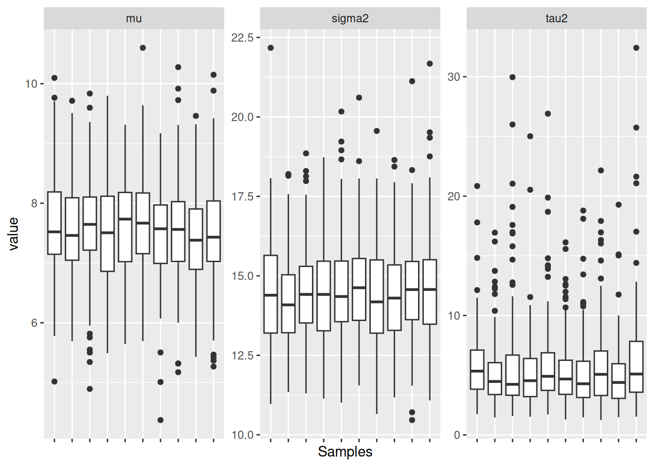
Assess convergence with diagnostic boxplots:
```{r echo=FALSE}
smt.df = data.frame(SMT)
colnames(smt.df) = c('sigma2', 'mu', 'tau2')
smt.df$s = 1:S
cut_size = 10
smt.df = smt.df %>%
tbl_df %>%
mutate(scut = cut(s, breaks = cut_size)) %>%
pivot_longer(cols = c(sigma2, mu, tau2), names_to = 'variable', values_to = 'value')
ggplot(smt.df, aes(x = scut, y = value)) +
facet_wrap(~ variable, scales = 'free_y') +
geom_boxplot() +
theme(axis.text.x = element_blank()) +
xlab('Samples')
```
Evaluate effective sample size:
```{r}
# Tweak number of samples until all of the below are above 1000
library(coda)
effectiveSize(SMT[, 1])
effectiveSize(SMT[, 2])
effectiveSize(SMT[, 3])
```
### b
Posterior means and confidence intervals
```{r}
t(apply(SMT, MARGIN = 2, FUN = quantile, probs = c(0.025, 0.5, 0.975)))
```
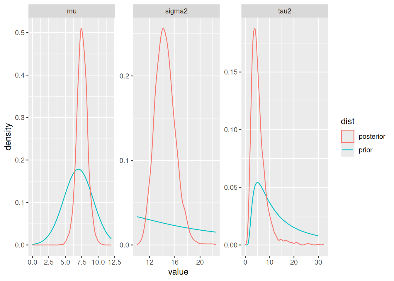
Comparing posterior to prior:
```{r}
# For dinvgamma
library(MCMCpack)
sigma2_prior = data.frame(
  value = seq(10, 22.5, by = 0.1),
  density = dinvgamma(seq(10, 22.5, by = 0.1), nu0 / 2, nu0 * s20 / 2),
  variable = 'sigma2'
)
tau2_prior = data.frame(
  value = seq(0, 30, by = 0.1),
  density = dinvgamma(seq(0, 30, by = 0.1), eta0 / 2, eta0 * t20 / 2),
  variable = 'tau2'
)
mu_prior = data.frame(
  value = seq(0, 12, by = 0.1),
  density = dnorm(seq(0, 12, by = 0.1), mu0, sqrt(g20)),
  variable = 'mu'
)
priors = rbind(sigma2_prior, tau2_prior, mu_prior)
priors$dist = 'prior'
smt.df$dist = 'posterior'

ggplot(priors, aes(x = value, y = density, color = dist)) +
  geom_line() +
  geom_density(data = smt.df, mapping = aes(x = value, y = ..density..)) +
  facet_wrap(~ variable, scales = 'free')
```
The prior estimates for $\mu$ and $\tau^2$ were fairly accurate, but the
estimate for $\sigma^2$ was very far off. After this analysis, estimates are obtained
for $\mu$, the average amount of hours of schoolwork spent at a typical school,
$\tau^2$, the variability between schools in the average hours of schoolwork,
and $\sigma^2$, the variability among students' hours in each school.
### c
```{r}
t20_prior = (1 / rgamma(1e6, eta0 / 2, eta0 * t20 / 2))
s20_prior = (1 / rgamma(1e6, nu0 / 2, nu0 * s20 / 2))

R_prior = data.frame(
  value = (t20_prior) / (t20_prior + s20_prior),
  dist = 'prior'
)
R_post = data.frame(
  value = SMT[, 'tau2'] / (SMT[, 'tau2'] + SMT[, 'sigma2']),
  dist = 'posterior'
)

ggplot(R_prior, aes(x = value, y = ..density.., color = dist)) +
  geom_density(data = R_prior) +
  geom_density(data = R_post)
mean(R_post$value)
```
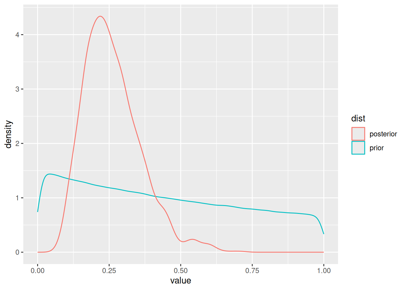
$R$ measures how much of the total variance in the data is between-group. The
prior didn't contain much information about this quantity, but after inference,
the expectation is that around 25\% of the variance comes from between group variance
($\tau^2$).
### d
```{r}
theta7_lt_6 = THETA[, 7] < THETA[, 6]
mean(theta7_lt_6)
theta7_smallest = (THETA[, 7] < THETA[, -7]) %>%
apply(MARGIN = 1, FUN = all)
mean(theta7_smallest)
```
### e
```{r}
relationship = data.frame(
  sample_average = ybar,
  post_exp = colMeans(THETA),
  school = 1:length(ybar)
)
ggplot(relationship, aes(x = sample_average, y = post_exp, label = school)) +
  geom_text() +
  geom_abline(slope = 1, intercept = 0) +
  geom_hline(yintercept = mean(schools.raw[, 'hours']), lty = 2) +
  annotate('text', x = 10, y = 7.9, label = paste0("Pooled sample mean ", round(mean(schools.raw[, 'hours']), 2))) +
  geom_hline(yintercept = mean(SMT[, 'mu']), color = 'red') +
  annotate('text', x = 10, y = 7.4, label = paste0("Posterior exp. mu ", round(mean(SMT[, 'mu']), 2)), color = 'red')
```
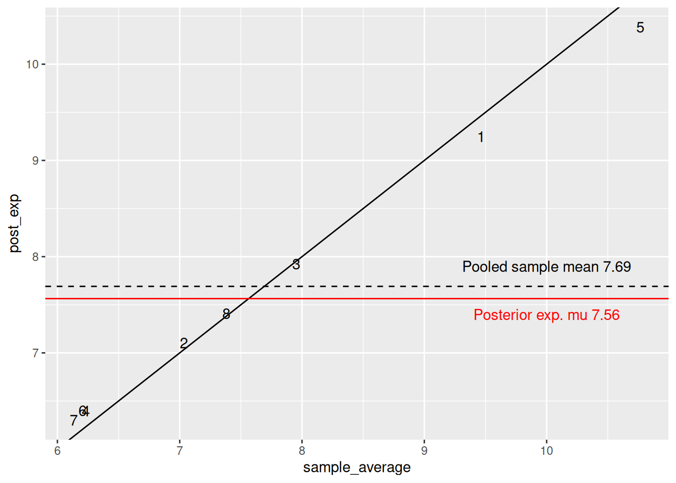
There is a quite tight correspondence between the sample average and the
posterior expectation, although mild shrinkage can be observed with schools with
very high and low sample averages being pulled towards the mean.