Chapter 4: Monte Carlo approximation
Why Monte Carlo? Often we want to calculate either arbitrary properties of posterior distributions or complex posterior distributions themselves. Often, clean analytical solutions for posterior distributions are difficult to obtain. By using computational methods, we can approximate arbitrarily complex posterior probability calculations by repeatedly sampling posteriors. Such techniques are known as Monte Carlo methods.
1 The Monte Carlo method
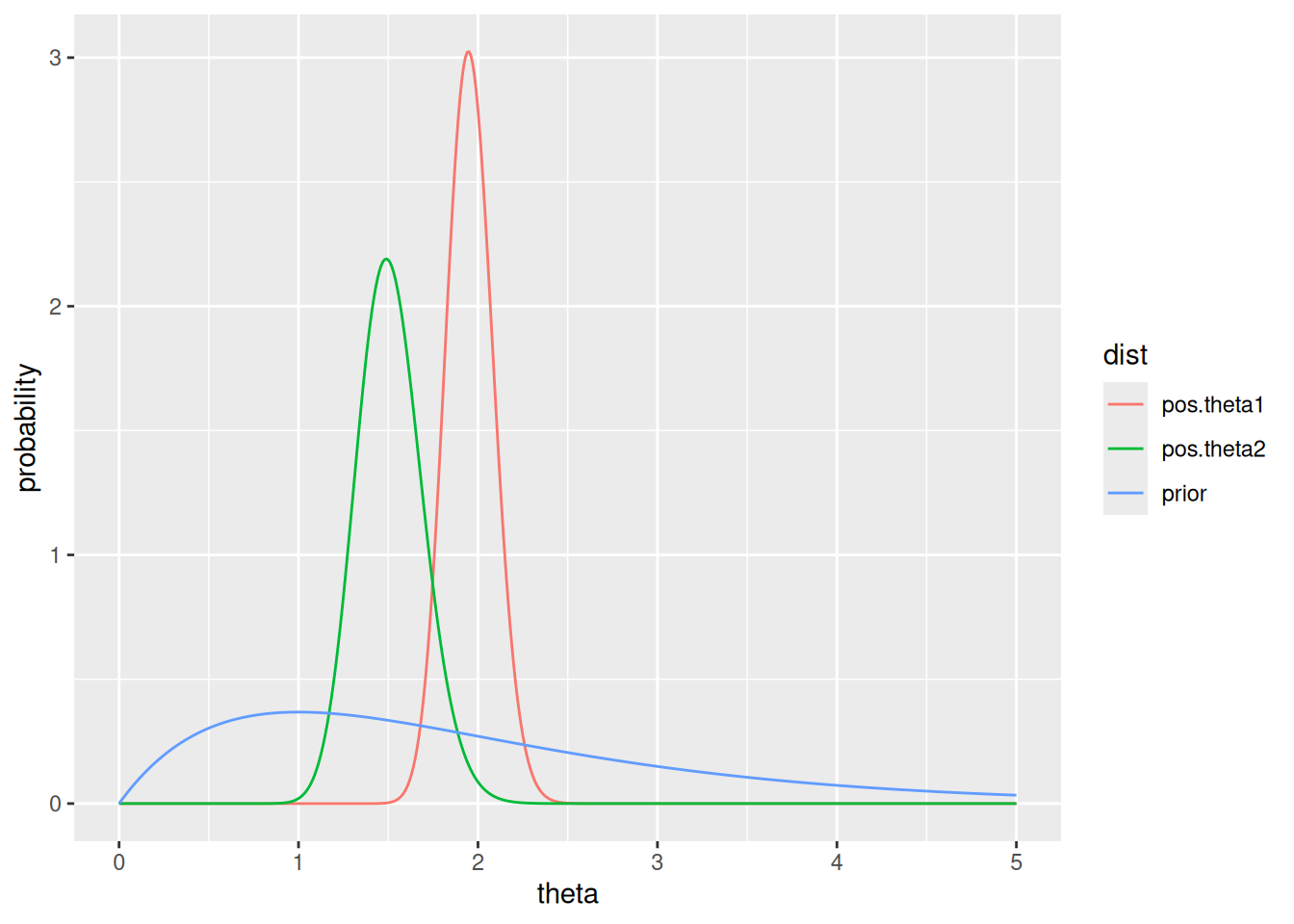
We continue the last chapter, where we found posterior distributions for women without (\(\theta_1\)) and with bachelor’s degrees (\(\theta_2\)). Recall
\[\begin{align} \left(\theta_1 \;\middle|\; \sum_i Y_{i, 1} = 217\right) &\sim \text{Gamma}(219, 112) \\ \left(\theta_2 \;\middle|\; \sum_i Y_{i, 2} = 217\right) &\sim \text{Gamma}(68, 45) \end{align}\]
To calculate the probability under these models that the mean number of children of women without bachelor’s degrees are higher than the mean number of those with bachelor’s degrees \(P(\theta_1 > \theta_2 \mid \dots)\), we can do so analytically. Notice that since \(\theta_1\) and \(\theta_2\) are independent, \(p(\theta_1, \theta_2) = p(\theta_1) p(\theta_2)\). If we plot \(\theta_1\) and \(\theta_2\) on the cartesian coordinate plane, the line \(\theta_1 = \theta_2\) divides two regions of the plane - one where \(\theta_1 > \theta_2\), the other where \(\theta_2 > \theta_1\). We double-integrate the joint density \(p(\theta_1, \theta_2)\) over the region we’re interested in.
Since for this example, the supports of \(\theta_1\) and \(\theta_2\) are \([0, \infty]\), we integrate over a portion of that region up to the line \(\theta_1 = \theta_2\):
\[\begin{align} P(\theta_1 > \theta_2 \mid y) &= \int_0^\infty \left( \int_0^{\theta_1} p(\theta_1 \mid y) p(\theta_2 \mid y) \; d\theta_2 \right) \; d\theta_1 \\ &= \int_0^\infty \left( \int_0^{\theta_1} \text{dgamma}(\theta_1, 219, 112) \times \text{dgamma}(\theta_2, 68, 45) \; d\theta_2 \right) \; d\theta_1 \\ \end{align}\]
Since Gamma distributions have well-defined PDFs, in this case the integral is computable and is reasonably easy in R:
However, when inference gets complicated, integrals may not be tractable. Alternatively, we can estimate via Monte Carlo estimation.
Notice that we can implement computational tools that allow us to sample arbitrarily from the Gamma distributions of \(\theta_1\) and \(\theta_2\). The details of implementing these samplers, i.e. functions that can draw some \(\theta_i \sim p(\theta \mid y)\), are non-trivial - for an example of algorithmically sampling from a Normal distribution given just pseudo-random number generators, see the Box-Muller transform (Goodman 2005). However, we will assume that we have these functions implemented. For example, in R we can represent \(n\) random draws from a gamma distribution with parameters \(a\) and \(b\) with the function call rgamma(n, a, b).
The law of large numbers states that, for \(S\) i.i.d. draws \(\theta^1, \dots, \theta^S\) from a distribution \(p(\theta)\), as \(S \rightarrow \infty\), \(\frac{1}{S} \sum \theta^i \rightarrow \mathbb{E}(p(\theta))\). This also implies that the variance of the sample approaches the variance of the distribution (to calcualte this, expand the formula for the variance of \(\theta\) into a combination of expectations, then use the law of large numbers of the expectations).
Indeed, by a more advanced theorem known as the Glivenko-Cantelli Lemma, the empirical distribution function of \(\theta^1, \dots, \theta^S\) approaches \(p(\theta)\). So more generally, we can approximate any quantity of interest of \(p(\theta)\) to arbitrary precision using a large enough sample from that function. This is visible in the image below, which demonstrates how the histogram and kernel density estimates of larger and large samples from the \(\theta_2 \sim \text{Gamma}(68, 45)\) distribution approach the distribution itself. In each panel, the true distribution is the dotted blue line.
Show R code
a = 68
b = 45

std.gamma = data.frame(theta = seq(0, 3, by = 0.01), p = dgamma(seq(0, 3, by = 0.01), a, b))
mc10 = data.frame(theta = rgamma(10, a, b), type = '10 samples')
mc100 = data.frame(theta = rgamma(100, a, b), type = '100 samples')
mc1000 = data.frame(theta = rgamma(1000, a, b), type = '1000 samples')

mcs = rbind(mc10, mc100, mc1000)

ggplot(mcs, aes(x = theta, y = ..density..)) +
  geom_histogram(bins = 10, fill = NA, color = 'black') +
  stat_density(fill = NA, color = 'black') +
  scale_x_continuous(limits = c(1, 2)) +
  geom_line(data = std.gamma, mapping = aes(x = theta, y = p), lty = 2, color = 'blue') +
  ylab('density') +
  facet_grid(. ~ type)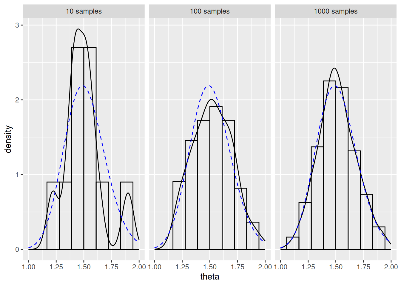
1.1 Numerical evaluation
The actual posterior mean of \(\theta_2 \mid y\) is \(68/45 = 1.51\). Notice we can approximate this mean with the mean of the above
Show R code
| Estimate of E(theta) | |
|---|---|
| 10 samples | 1.497037 |
| 100 samples | 1.518160 |
| 1000 samples | 1.516626 |
We can calculate probabilities of events concerning theta by counting the number of times in our sample the randomly sampled value satisfies the event. For example, to calculate \(P(\theta < 1.75 \mid y)\), we observe the number of times a sampled \(\theta^{i} < 1.75\). In R, comparison operators like > or == operate element-wise, so mc1000$theta < 1.75 returns a boolean vector of Ts and Fs depending on whether the specific \(\theta^i\) is indeed less than 1.75:
Thus, we can calculate
Show R code
| Estimate of P(theta < 1.75) | |
|---|---|
| 10 samples | 0.900 |
| 100 samples | 0.920 |
| 1000 samples | 0.895 |
Notice the true probability can be calculated with via pgamma(1.75, 68, 45) and is 0.9.
1.2 Convergence
We can measure how quickly our estimates converge to the true mean (for this example, when the true mean is known) by plotting the estimate thus far as the number of samples in our estimation increase, as below:
Show R code
cstats = data.frame(
  n = seq_along(mc1000$theta),
  'Expectation' = cumsum(mc1000$theta) / seq_along(mc1000$theta),
  'Probability' = cumsum(mc1000$theta < 1.75) / seq_along(mc1000$theta < 1.75)
) |>
  pivot_longer(cols = -n, names_to = 'variable', values_to = 'value')
realstats = data.frame(
  stat = c(68 / 45, pgamma(1.75, 68, 45)),
  variable = c('Expectation', 'Probability')
)
ggplot(cstats, aes(x = n, y = value)) +
  facet_wrap(~ variable, scales = 'free') +
  geom_line() +
  ylab('Estimate') + xlab('Number of samples') +
  geom_hline(data = realstats, mapping = aes(yintercept = stat), lty = 2)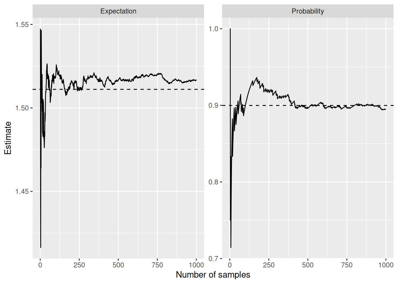
Since, due to the central limit theorem, estimates of the mean of \(\theta^1, \dots, \theta^S\) (and other quantities??) are approximately normally distributed for large \(S\), we can construct confidence intervals for our estimates based on the sample size.
Specifically, an approximate 95% confidence interval for \(\theta\) is
\[ \hat{\theta} \pm 1.96 \sqrt{\hat{\sigma}^2 / S} \]
where \(\hat{\sigma}^2\) is the unbiased estimator of the population variance (hence the approximate confidence interval; divide by \(S - 1\), not \(S\)). Using this, we can estimate the number of samples we ought to take to report our estimate to a certain degree of precision. We ought to take enough samples such that the standard error \(\sqrt{\hat{\sigma}^2/S} < \alpha\) where \(\alpha\) is the desired level of precision. Of course, since we don’t know how variable our samples are, we don’t know how big \(\hat{\sigma}^2\) is, so we cannot a priori determine the number of samples to run. It is possible, however, to run a smaller number of samples first to determine an estimate of \(\hat{\sigma}^2\) and thus the standard error, then conservatively use that estimate to identify the size of \(S\) required for the desired precision.
2 Posterior inference for arbitrary functions
If we can sample \(\theta^{(1)}, \dots, \theta^{(S)} \sim p(\theta \mid y)\) i.i.d., then we can obtain distributions for any arbitrary function \(g(\theta)\). We just need to sample \(S\) \(\theta^{(i)}\), then apply \(g\) to each \(\theta^{(i)}\) to obtain the value of interest, say \(\gamma^{(i)}\). This step is deterministic, so we are actually sampling from \(p(\gamma \mid y)\). Thus, by the sample law of large numbers and central limit theorem derivations as before, Monte Carlo estimations can estimate arbitrary functions to any degree of accuracy. This is very powerful and flexible!
2.1 Example: Log-odds
Log-odds is the relative likelihood that an event with probability \(\theta\) will occur versus not occur. Specifially,
\[\begin{align} \text{log odds}(\theta) = \log \left( \frac{\theta}{1 - \theta} \right) = \gamma. \end{align}\]
If \(\theta = 0.5 = 1 - \theta\) then \(\text{log odds}(\theta) = 0\). If \(\theta\) is more likely to happen than not, then \(\text{log odds}(\theta) > 0\). If \(\theta\) is less likely to happen than not, then \(\text{log odds}(\theta) < 0\).
We return to surveys. Imagine we survey 860 individuals about agreement with a recent Supreme Court ruling and \(y = 441\) say they agreed with the ruling. Say we have a uniform prior on \(\theta\) before observing any data, so \(\theta \sim \text{Beta}(1, 1)\).
Notice that, even when given a concrete prior distribution, calculating the prior distribution on \(\gamma\) requires actual calculations. They may be managable in this case, but the point is that as functions become far more complicated than the log-odds calculation in this example, even computing a closed form for our prior may be intractable.
So we can do Monte Carlo estimation of prior and posterior distributions of \(\gamma\) based on our knowledge about how \(\theta\) updates after observing data. Recall that, in our beta-binomial model, if \(\theta \sim \text{Beta}(a, b) = \text{Beta}(1, 1)\), then \(\theta \mid y_1, \dots, y_n \sim \text{Beta}(a + n, b + n - y) = \text{Beta}(442, 420)\).
Notice that our log odds ratio is quite close to 0. Moreover, by leveraging Monte Carlo estimation, we are very (approximately) precise about the precise shape of our prior and posterior distributions, with little mathematical derivation required.
Show R code
a = 1
b = 1
y = 441
n = 860
n.samp = 10000

log.odds = function(x) log(x / (1 - x))

theta.prior.mc = rbeta(n.samp, a, b)
# Now compute gammas as a function of theta!
prior = log.odds(theta.prior.mc)

theta.post.mc = rbeta(n.samp, a + y, b + n - y)
posterior = log.odds(theta.post.mc)

combined = as.data.frame(cbind(prior, posterior)) |>
  tibble::rownames_to_column('n') |>
  pivot_longer(cols = -n, names_to = 'type', values_to = 'value')

ggplot(combined, aes(x = value, group = type, color = type)) +
  geom_density(fill = NA) +
  scale_x_continuous(limits = c(-5, 5)) +
  xlab('gamma')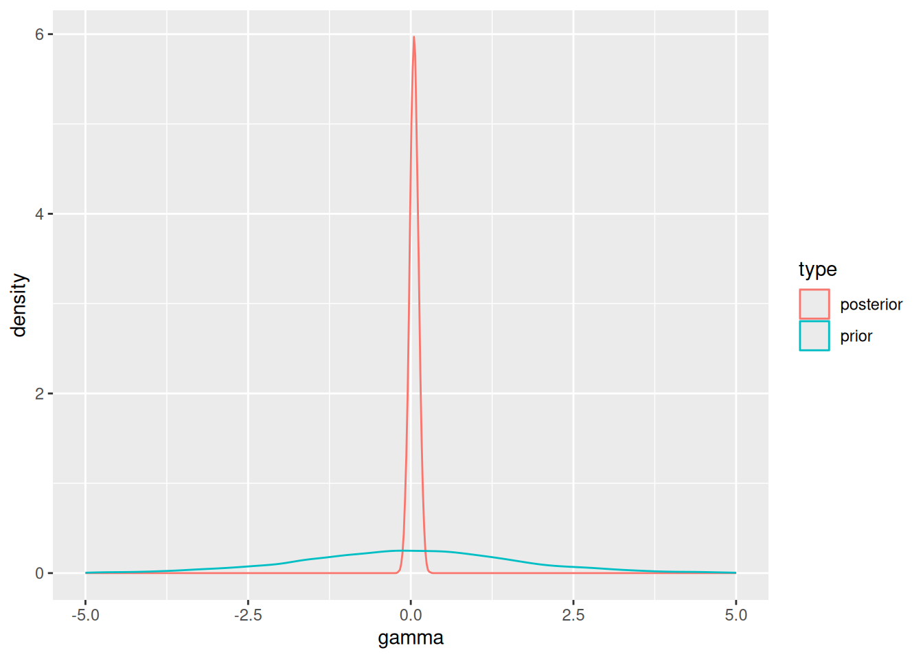
2.2 Example 2: Functions of two parameters
We can now return back to the earlier example with two separate Poisson models of the number of children of women’s without and with bachelor’s degrees. Since \(\theta_1\) and \(\theta_2\) are independent, we can sample a pair \((\theta^{(i)}_1, \theta^{(i)}_2)\) from separate samples from \(p(\theta_1 \mid y)\) and \(p(\theta_2 \mid y)\), such that many such pairs \((\theta^{(i)}_1, \theta^{(i)}_2)\) will (by Monte Carlo estimation) approximate the joint density of \(p(\theta_1, \theta_2)\) without needing to calculate or integrate over the joint density by hand. Again,
\[\begin{align} \left(\theta_1 \;\middle|\; \sum_i Y_{i, 1} = 217\right) &\sim \text{Gamma}(219, 112) \\ \left(\theta_2 \;\middle|\; \sum_i Y_{i, 2} = 217\right) &\sim \text{Gamma}(68, 45) \end{align}\]
the corresponding derivation is thus
Also, like the gamma example above, we can calculate some arbitrary function. Say we are interested in the ratio \(f(\theta_1, \theta_2) = \theta_1/\theta_2\) of the means. On average, how many times more children do women without bachelor’s degrees have compared to those with bachelor’s degrees. Then we sample multiple pairs \((\theta^{(i)}_1, \theta^{(i)}_2)\), and multiple pairs \(\gamma^i = f(\theta^{(i)}_1, \theta^{(i)}_2)\).
Show R code
# Common prior
a = 2
b = 1
# Without bachelor's
n1 = 111
y1 = 217
# With
n2 = 44
y2 = 66

n.samp = 10000

ratio = function(a, b) a / b # Not necessary, but good for foramlization

# Approximate prior distribution for good measure
prior = ratio(rgamma(n.samp, a, b), rgamma(n.samp, a, b))
posterior = ratio(rgamma(n.samp, a + y1, b + n1), rgamma(n.samp, a + y2, b + n2))

combined = as.data.frame(cbind(prior, posterior)) |>
  tibble::rownames_to_column('n') |>
  pivot_longer(cols = -n, names_to = 'type', values_to = 'value') |>
  mutate(type = factor(type, levels = c('prior', 'posterior')))

ggplot(combined, aes(x = value, group = type, color = type)) +
  facet_wrap(~ type, scales = 'free_y') +
  scale_x_continuous(limits = c(0, 10)) +
  geom_density(fill = NA) +
  xlab(expression(theta[1] / theta[2]))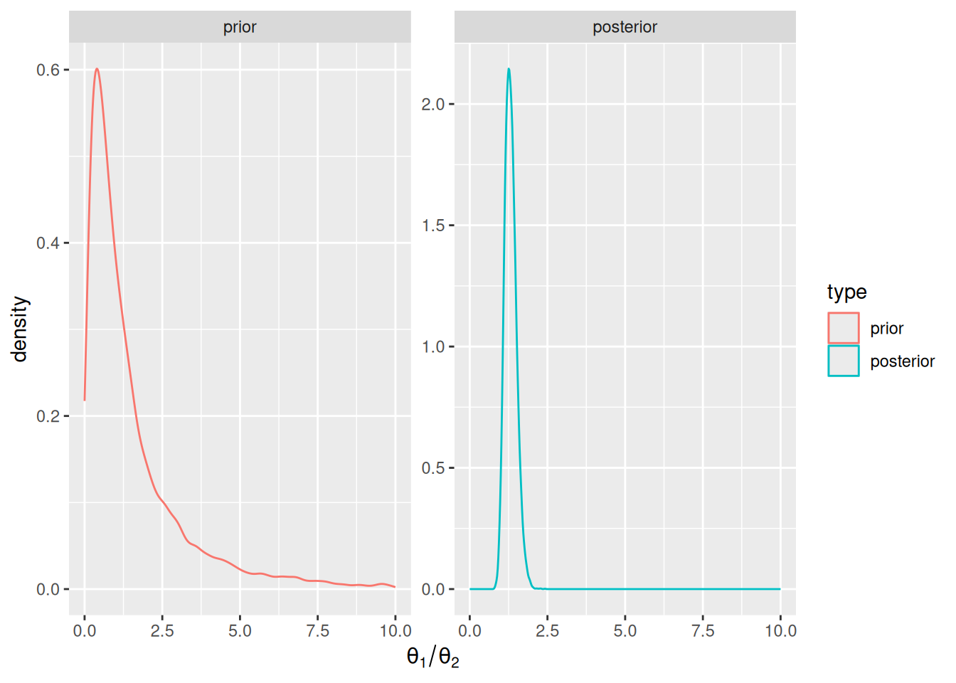
3 Sampling from predictive distributions
Recall that predictive distributions are distributions of new realizations of a random variable when existing data have been conditioned on and unknown quantities (i.e. parameters) are integrated out.
For example, given a prior distribution \(p(\theta)\), how can we calculate the prior predictive distribution \(p(\tilde{y})\)? Often we have an analytical solution for the form a posterior predictive distribution for a given model. But often we can simply sample many \(\theta^{(i)}\) from our posterior distribution on \(\theta\), and then sample a \(y^{(i)}\) for each \(\theta^{(i)}\). Specifically, \(\{(\theta, \tilde{y}) \}^{(1)}, \dots, (\theta, \tilde{y})^{(S)} \}\) are samples from the joint posterior distribution of \(\theta, \tilde{Y}\), and the sequence \(\{\tilde{y}^{(1)}, \dots, \tilde{y}^{(S)}\}\) are samples from the marginal posterior distribution of \(\tilde{Y}\) (if we had an infinite number of samples, we would be “summing” over all theta).
4 Posterior predictive model checking
Because exercises 4.3 and 4.8 address this, this section is skipped for now.
5 Exercises
5.1 4.1
For the county in exercise 3.1, \(\theta_3 \mid \sum Y_i = y \sim \text{Beta}(58, 44)\).
For this county, assuming a uniform prior, \(\theta_4 \mid \sum Y_i = y \sim \text{Beta}(31, 21)\).
So,
5.2 4.2
5.2.1 a
5.2.2 b
Show R code
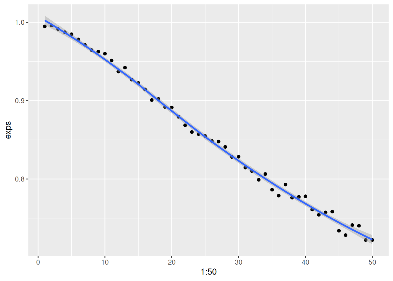
Even a strong factor of \(n_0\) has a relatively minimal effect on the posterior distribution.
5.2.3 c
Recall for a Poisson model, the posterior predictive distribution after a \(\text{Gamma}(a, b)\) prior is a negative binomial distribution \(\text{NB}(a + \sum y_i, b, n)\). (The posterior predictive parameters are the same as those of the posterior distribution itself). However, we can also simulate it by sampling from the Poisson distribution implied by the sampled theta.
Show R code
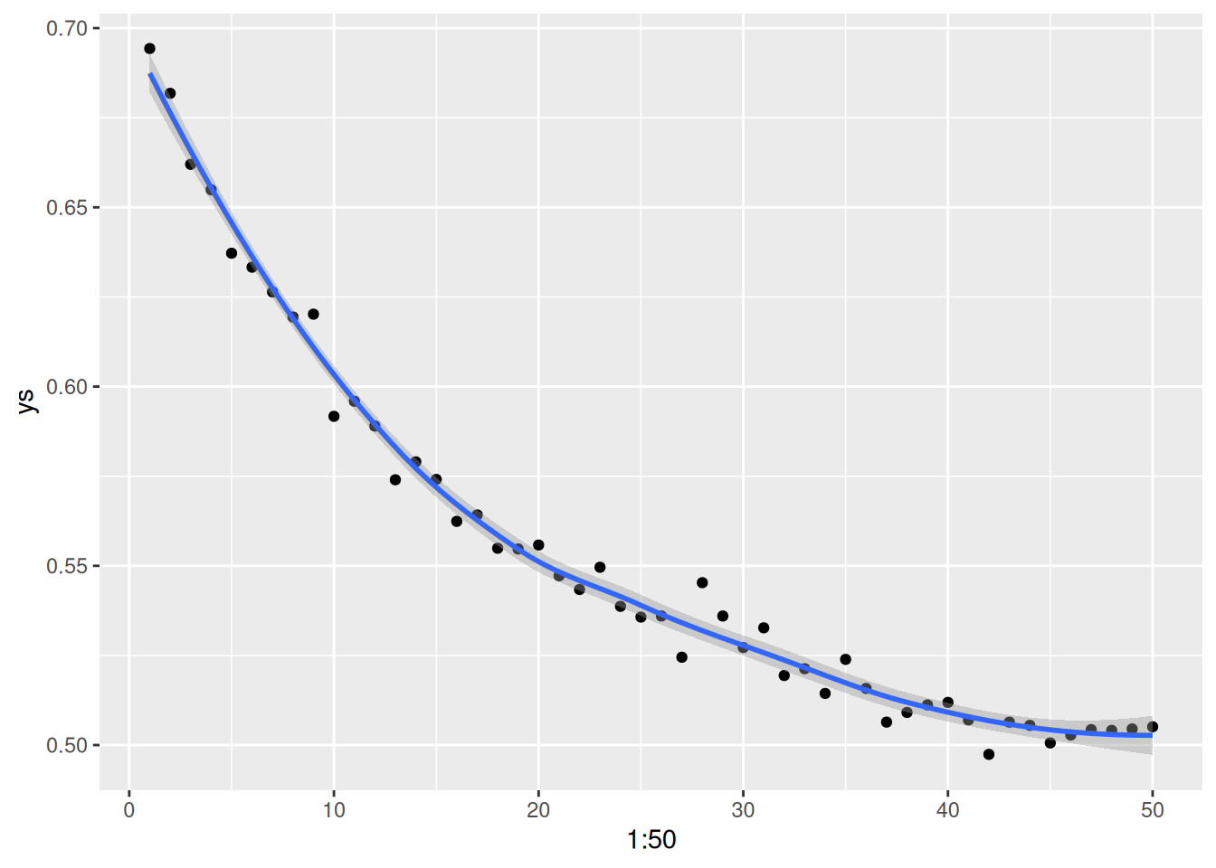
Which appears to be a different relationship - exactly what it is could be calculated by integrating the quantity using the posterior distribution, then figuring out what the shape is as a function of \(n_0\).
5.3 4.3
5.3.1 a
Using ya:
Show R code
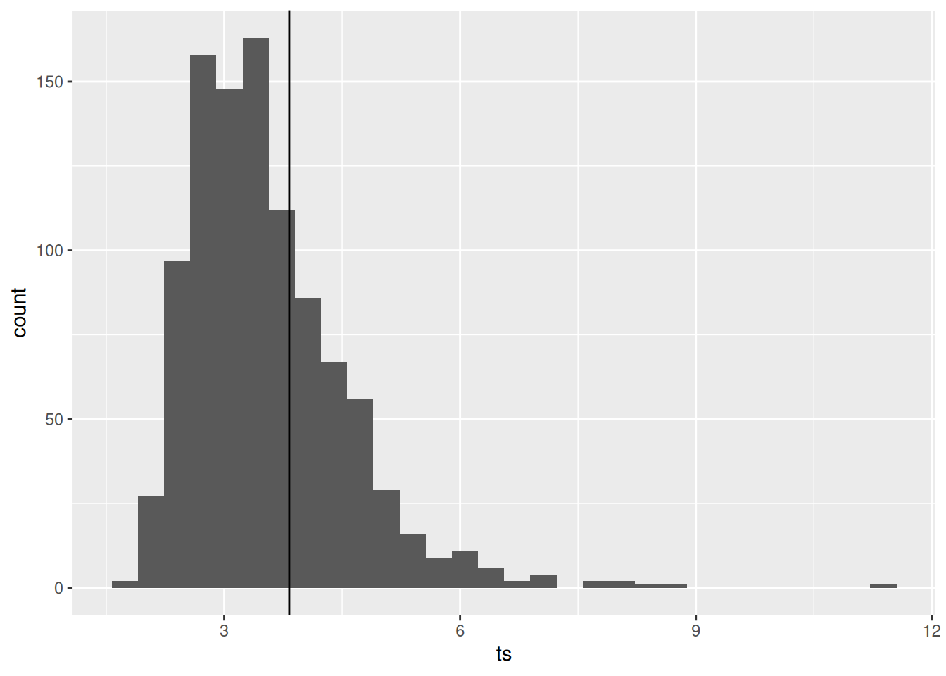
Since the observed statistic (vertical line) is centered well within the standard spread of the observed \(t(s)\), we have no reason to believe the fit of the Poisson model is bad. Also, since \(t(s)\) depends on the only parameter of the data \(\theta\), it can thus be inferred that the Poisson model seems to fit reasonably in this case.
5.3.2 b
Using yb:
Show R code
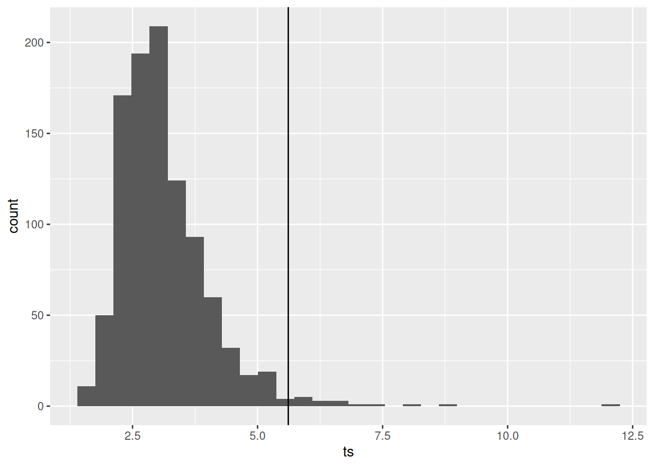
Since the observed statistic (vertical line) seems to be an outlier for the range of statistics normally seen in this dataset, we can infer that the Poisson model does not seem to fit this dataset well.
5.4 4.6
5.4.1 via Monte-Carlo sampling
Show R code
theta.mc = runif(10000)
gamma.mc = sapply(theta.mc, function(theta) log(theta / (1 - theta)))
ggplot(data.frame(gamma = gamma.mc), aes(x = gamma, y = ..density..)) +
  geom_histogram()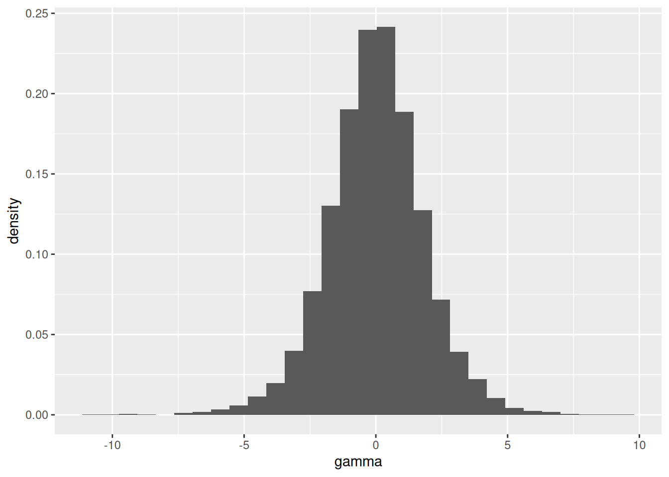
Yes, the prior for \(\gamma\) is centered around 0 and appears to be normally distributed. Naturally, \(p(\gamma)\) must be centered around something, since you cannot have a uniform distribution on an infinite interval.
5.4.2 analytically
This is computed in Exercise 3.10 (a).
5.5 4.7
5.5.1 a
We first sample \((\theta, \sigma^2)\) via sampling from \(p(\sigma^2)\) and then \(p(\theta \mid \sigma^2)\):
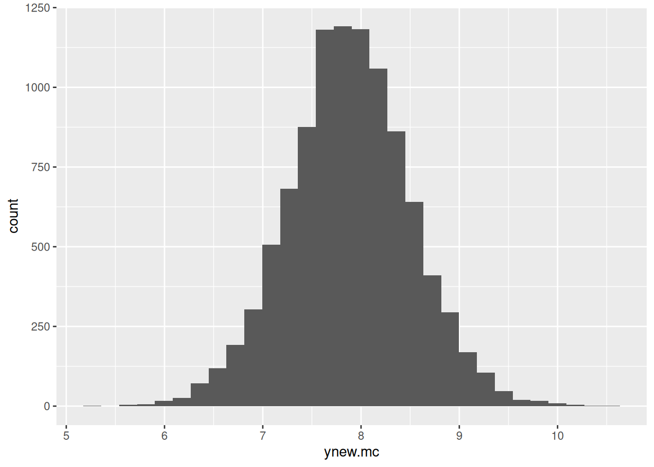
Now we can sample according to the mixture posterior distribution:
5.5.2 b
5.5.3 c
Show R code
# i. Compute and normalize density
dens = density(ynew.mc)
dens.ynorm = dens$y / sum(dens$y)
# ii. Sort in decreasing order
dens.ynorm.desc = dens.ynorm[order(dens.ynorm, decreasing = TRUE)]
# iii. Find first probability value st cumsum of sorted values > 0.75
cutoff = dens.ynorm.desc[min(which(cumsum(dens.ynorm.desc) > 0.75))]
in.hdp = dens.ynorm > cutoff
ggplot(data.frame(y = dens$x, density = dens.ynorm, hdp = in.hdp)) +
  geom_point(aes(x = y, y = density, color = hdp))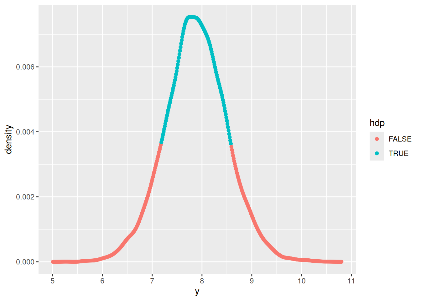
Since the distribution of weights is relatively symmetric and normally distributed, the HDP and quantile confidence intervals are quite similar.
5.5.4 d
Perhaps a combination of multiple parts of a vegetable which have known distributions (e.g. stem, fruit, leaves, etc)
5.6 4.8
5.6.1 a
Show R code
a = 2
b = 1
N = 5000

thetaA = rgamma(N, a + sum(menchild30bach), b + length(menchild30bach))
thetaB = rgamma(N, a + sum(menchild30nobach), b + length(menchild30nobach))

ynewA = rpois(N, thetaA)
ynewB = rpois(N, thetaB)

pos.predict = data.frame(
  ynew = c(ynewA, ynewB),
  dist = factor(rep(c('bach', 'nobach'), each = N), levels = c('bach', 'nobach')),
  type = 'posterior'
)
ggplot(pos.predict, aes(x = ynew, group = dist)) +
  geom_histogram() +
  facet_grid(. ~ dist)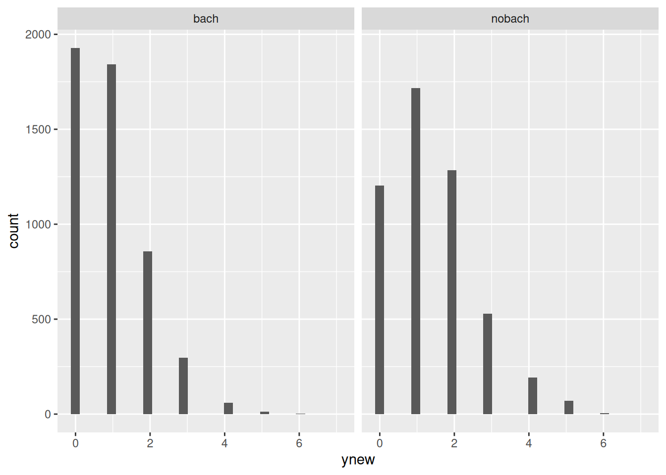
5.6.2 b
Show R code
theta.diff = thetaB - thetaA
print("Theta difference:")
#> [1] "Theta difference:"
print(quantile(theta.diff, c(0.025, 0.975)))
#>      2.5%     97.5%
#> 0.1530478 0.7364150

ynew.diff = ynewB - ynewA
print("Ynew difference:")
#> [1] "Ynew difference:"
print(quantile(ynew.diff, c(0.025, 0.975)))
#>  2.5% 97.5%
#>    -2     4
Since the confidence interval for \(\theta_B - \theta_A\) does not contain zero, we believe with at least approximately 95% probability that the true posterior mean \(\theta_B\) is greater than \(\theta_A\). However, the same does not hold true for the means of the difference between two individuals sampled from this distribution, due to the increased uncertainty in the posterior predictive distribution.
5.6.3 c
Show R code
emp.df = data.frame(
  ynew = c(menchild30bach, menchild30nobach),
  dist = factor(c(rep('bach', length(menchild30bach)), rep('nobach', length(menchild30nobach))), levels = c('bach', 'nobach')),
  type = 'empirical'
)

total.df = rbind(pos.predict, emp.df)

ggplot(total.df, aes(x = ynew, y = ..density.., group = type, fill = type)) +
  geom_histogram(position = 'dodge') +
  facet_grid(. ~ dist)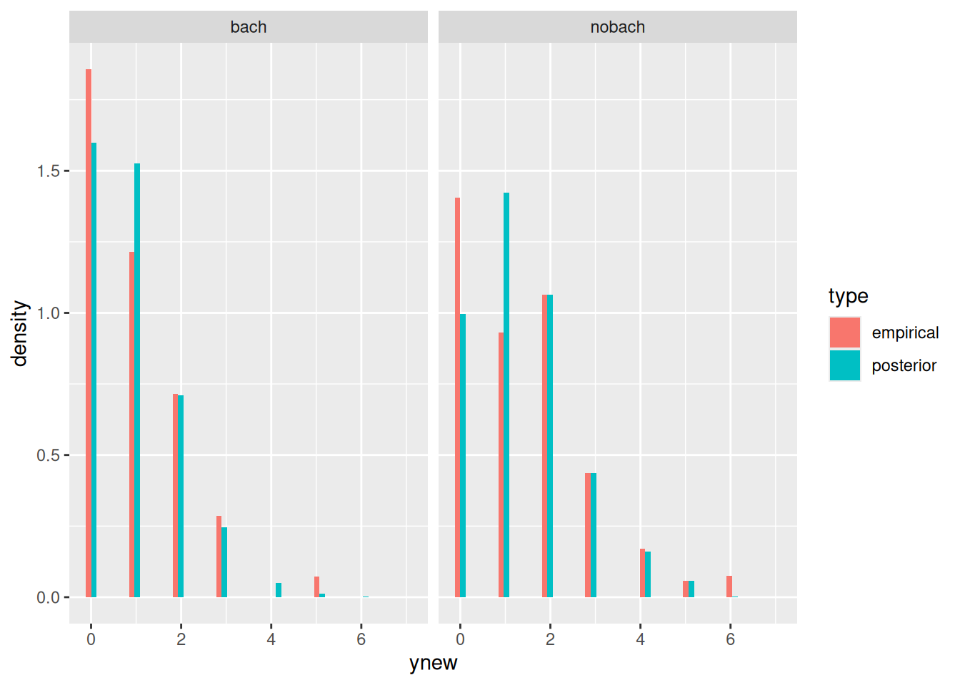
The posterior distribution for \(\tilde{Y}_B\) seems to peak around 1, while the empirical distribution peaks strongly around 0. This suggests an error in the model fit.
(Observe that the mean of the nobach population is around 1.4)
Show R code
mean(ynewB)
#> [1] 1.4038
5.6.4 d
Model checking, by computing a statistic that may be of interest:
Show R code
zeroandone = lapply(thetaB, function(theta) {
  nB = rpois(218, theta)
  n0s = sum(nB == 0)
  n1s = sum(nB == 1)
  c(n0s, n1s)
})
zeros = sapply(zeroandone, function(t) t[1])
ones = sapply(zeroandone, function(t) t[2])
ggplot(data.frame(zeros = zeros, ones = ones)) +
  geom_point(aes(x = zeros, y = ones), alpha = 0.1) +
  annotate('point', x = sum(menchild30nobach == 0), y = sum(menchild30nobach == 1), color = 'red')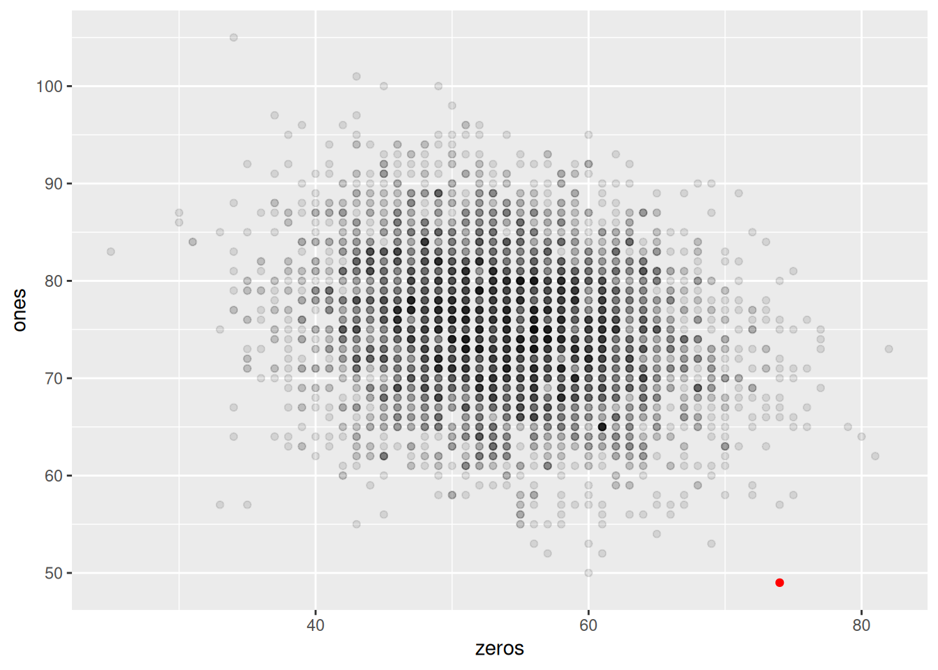
The observed statistic is in red. Notice how it seems somewhat abnormal for sample datasets from our poisson model with \(\theta = 1.4\) especially in the case of the number of ones observed. This is a clear indicator that the fit of our Poisson model is suboptimal.
References
Goodman, Jonathan. 2005. “Gaussian Sampling.” http://www.math.nyu.edu/faculty/goodman/teaching/MonteCarlo2005/notes/GaussianSampling.pdf.