Show R code
swim = read.table('Exercises/swim.dat')swim = read.table('Exercises/swim.dat')To specify the prior, the prior expectation of the \(y\)-intercept is set to 23, and the prior expectation of the effect of training week by week is set to 0, so \(\boldsymbol{\beta} = (23, 0)^T\).
No covariance with the \(\beta\) coefficients is expected, but there is uncertainty about the initial \(\beta\) estimates. Specifically, to let 95% of the uncertainty of the \(y\)-intercept fall in \([22, 24]\), \(\Sigma_{0(1, 1)} = 1/4\) is set (so that \(\pm\) 2 standard deviations is \(\pm\) 1). Training is expected to have a relatively mild effect on time, so \(\Sigma_{0(2, 2)} = 0.1\) is set, which is an arbitrarily chosen small variance.
For the expectation of the variability of measurements, similarly set \(\sigma^2_0 = 1/4\) and only lightly center this prior with \(\nu_0 = 1\).
library(MASS) # mvrnorm
library(dplyr)
S = 5000
X = cbind(rep(1, 6), seq(1, 11, by = 2))
n = dim(X)[1]
p = dim(X)[2]

# Prior
beta0 = c(23, 0)
sigma0 = rbind(c(0.25, 0), c(0, 0.1))
nu0 = 1
s20 = 0.25

set.seed(1)

inv = solve

# For each swimmer, run linear regression gibbs sampling and obtain a posterior
# predictive distribution
swim_pred = apply(swim, MARGIN = 1, function(y) {

  # Store samples
  BETA = matrix(nrow = S, ncol = length(beta0))
  SIGMA = numeric(S)

  # Starting values - just use prior values?
  beta = c(23, 0)
  s2 = 0.7^2

  # Gibbs sampling algorithm from 9.2.1
  for (s in 1:S) {
    # 1a) Compute V and m
    V = inv(inv(sigma0) + (t(X) %*% X) / s2)
    m = V %*% (inv(sigma0) %*% beta0 + (t(X) %*% y) / s2)

    # 1b) sample beta
    beta = mvrnorm(1, m, V)

    # 2a) Compute SSR(beta) (specific formula from 9.1)
    ssr = (t(y) %*% y) - (2 * t(beta) %*% t(X) %*% y) + (t(beta) %*% t(X) %*% X %*% beta)

    # 2b) sample s2
    s2 = 1 / rgamma(1, (nu0 + n) / 2, (nu0 * s20 + ssr) / 2)

    BETA[s, ] = beta
    SIGMA[s] = s2
  }

  # Now sample posterior predictive - two weeks later
  xpred = c(1, 13)
  YPRED = rnorm(S, BETA %*% xpred, sqrt(SIGMA))

  YPRED
})With the posterior predictive dataset, swimmer 1 is the fastest about 65% of the time by week 13, so the recommendation is that swimmer 1 race.
crime = read.table('Exercises/crime.dat', header = TRUE)y = crime$y
X = crime %>% dplyr::select(-y) %>% as.matrix
n = dim(X)[1]
p = dim(X)[2]
g = n
nu0 = 2
s20 = 1
S = 1000
Hg = (g / (g + 1)) * X %*% inv(t(X) %*% X) %*% t(X)
SSRg = t(y) %*% (diag(1, nrow = n) - Hg) %*% y
s2 = 1 / rgamma(S, (nu0 + n) / 2, (nu0 * s20 + SSRg) / 2)
Vb = g * inv(t(X) %*% X) / (g + 1)
Eb = Vb %*% t(X) %*% y
E = matrix(rnorm(S * p, 0, sqrt(s2)), S, p)
beta = t(t(E %*% chol(Vb)) + c(Eb))library(tidyr)
signif = apply(beta, MARGIN = 2, FUN = quantile, probs = c(0.025, 0.5, 0.975)) %>%
apply(MARGIN = 2, FUN = function(y) !(y[1] < 0 && 0 < y[3]))
beta_df = as.data.frame(beta) %>%
pivot_longer(cols = everything(), names_to = 'variable', values_to = 'coefficient') %>%
mutate(signif = signif[variable])
ggplot(beta_df, aes(x = variable, y = coefficient, color = signif)) +
stat_summary(fun.y = mean, fun.ymin = function(y) quantile(y, probs = c(0.025)), fun.ymax = function(y) quantile(y, probs = c(0.975))) +
geom_hline(yintercept = 0, lty = 2)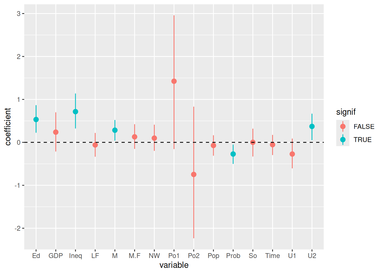
Looks like Ed (mean years of schooling), Ineq (Income inequality), M (percentage of males aged 14-24), Prob (probability of imprisonment), and U2 (unemployment rate of urban males 35-39).
# From 9.1
beta_ols = inv(t(Xtr) %*% Xtr) %*% t(Xtr) %*% ytr
beta_ols
#>             [,1]
#> M     0.19419790
#> So    0.20624856
#> Ed    0.64334998
#> Po1   0.30590821
#> Po2   0.44725441
#> LF   -0.09198965
#> M.F   0.03537926
#> Pop   0.08440462
#> NW   -0.01227990
#> U1   -0.03278782
#> U2    0.15494093
#> GDP   0.10455812
#> Ineq  0.76691166
#> Prob -0.25823362
#> Time  0.05938070

y_ols = Xte %*% beta_ols

ols_df = data.frame(
  observed = yte,
  predicted = y_ols
)

ggplot(ols_df, aes(x = observed, y = predicted)) +
  geom_point() +
  geom_smooth(method = 'lm')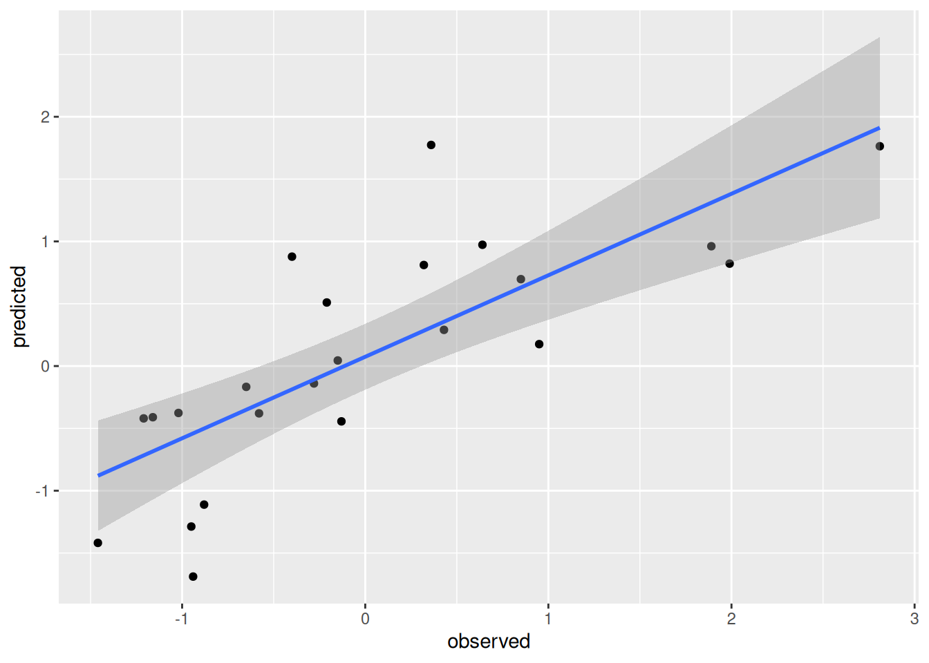
y = ytr
X = Xtr

n = dim(X)[1]
p = dim(X)[2]

g = n
nu0 = 2
s20 = 1

S = 1000

Hg = (g / (g + 1)) * X %*% inv(t(X) %*% X) %*% t(X)
SSRg = t(y) %*% (diag(1, nrow = n) - Hg) %*% y

s2 = 1 / rgamma(S, (nu0 + n) / 2, (nu0 * s20 + SSRg) / 2)
Vb = g * inv(t(X) %*% X) / (g + 1)
Eb = Vb %*% t(X) %*% y

E = matrix(rnorm(S * p, 0, sqrt(s2)), S, p)
beta = t(t(E %*% chol(Vb)) + c(Eb))

beta_bayes = as.matrix(colMeans(beta))

y_bayes = Xte %*% beta_bayes

bayes_df = data.frame(
  observed = yte,
  predicted = y_bayes
)

ggplot(ols_df, aes(x = observed, y = predicted)) +
  geom_point() +
  geom_smooth(method = 'lm')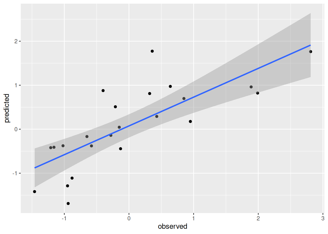
At least when the seed is 1, there doesn’t appear to be a major difference between the prediction errors.
# Unnecessary code repeating here. Clean this up later w/ functions
N = 100
set.seed(1)
pred_errors = t(sapply(1:N, function(i) {
  y = crime$y
  X = crime %>% dplyr::select(-y) %>% as.matrix
  train_i = sample.int(length(y), size = round(length(y) / 2), replace = FALSE)
  ytr = y[train_i]
  Xtr = X[train_i, ]
  yte = y[-train_i]
  Xte = X[-train_i, ]

  # OLS
  beta_ols = inv(t(Xtr) %*% Xtr) %*% t(Xtr) %*% ytr
  beta_ols

  y_ols = Xte %*% beta_ols

  pred_error_ols = sum((yte - y_ols)^2) / length(yte)

  # Bayes
  y = ytr
  X = Xtr

  n = dim(X)[1]
  p = dim(X)[2]

  g = n
  nu0 = 2
  s20 = 1

  S = 1000

  Hg = (g / (g + 1)) * X %*% inv(t(X) %*% X) %*% t(X)
  SSRg = t(y) %*% (diag(1, nrow = n) - Hg) %*% y

  s2 = 1 / rgamma(S, (nu0 + n) / 2, (nu0 * s20 + SSRg) / 2)
  Vb = g * inv(t(X) %*% X) / (g + 1)
  Eb = Vb %*% t(X) %*% y

  E = matrix(rnorm(S * p, 0, sqrt(s2)), S, p)
  beta = t(t(E %*% chol(Vb)) + c(Eb))

  beta_bayes = as.matrix(colMeans(beta))

  y_bayes = Xte %*% beta_bayes

  pred_error_bayes = sum((yte - y_bayes)^2) / length(yte)

  c(pred_error_ols, pred_error_bayes)
})) %>% as.data.frame
colnames(pred_errors) = c('ols', 'bayes')
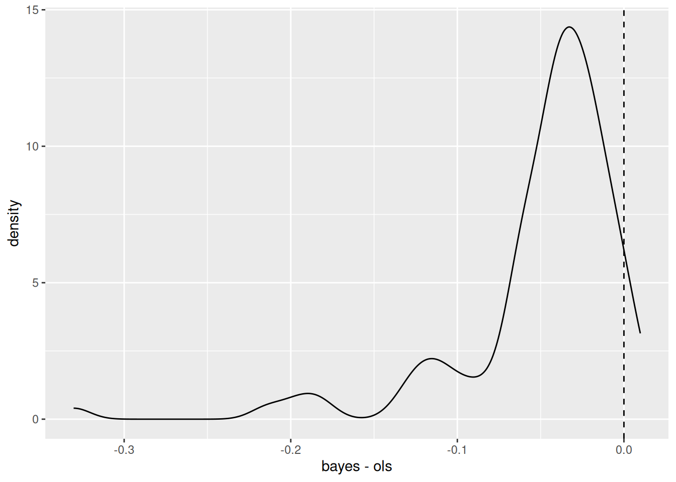
Here’s a plot of the density of \(\text{err}_{\text{Bayes}} - \text{err}_{\text{ols}}\). If this is less than 0, then the Bayes estimator did better than the OLS estimator:
Lastly,
mean(pred_errors$bayes < pred_errors$ols)
#> [1] 0.96
For N samples, 96% of the time, the predictive error using the Bayes estimators is less than the predictive error using the OLS estimators. Nice!